Continuous Opinion Dynamics: Insights through Interactive Markov Chains

ABSTRACT
We reformulate the agent-based opinion dynamics models of Weisbuch-Deffuant [1, 2] and Hegselmann-Krause [3] as interactive Markov chains. So we switch the scope from a finite number of $n$ agents to a finite number of $n$ opinion classes. Thus, we will look at an infinite population distributed to opinion classes instead of agents with real number opinions.

The interactive Markov chains show similar dynamical behavior as the agent-based models: stabilization and clustering. Our framework leads to a ’discrete’ bifurcation diagram for each model which gives a good view on the driving forces and the attractive states of the system. The analysis shows that the emergence of minor clusters in the Weisbuch-Deffuant model and of meta-stable states with very slow convergence to consensus in the Hegselmann-Krause model are intrinsic to the dynamical behavior.

KEY WORDS
continuous opinion dynamics, repeated averaging, bounded confidence

1 Introduction

Consider a certain number of agents discussing a certain issue. Each agent has an opinion about that issue and they try to find a consensus. The opinion should be representable as a real number. Thus, agents can compromise by averaging their opinions. We label such dynamics as continuous opinion dynamics. ’Continuous’ refers to the type of opinions not to the time. This is in contrast to several models of opinion dynamics which cover binary opinions where agents have to decide ’yes’ or ’no’.

Examples for continuous opinions are prices or the continuum form left to right in politics. Clusters of agents in the continuous opinion space may represent e. g. low-budget vs. luxury shoppers or political parties.

There are several more or less complex models concerning continuous opinion dynamics [4, 5, 6, 7]. The recently most discussed models are the models of Weisbuch-Deffuant (WD) [1] and Hegselmann-Krause (HK) [3]. Both models use very similar heuristics. We will present both models and focus on the dynamical differences in computer simulation.

In the third section we will define interactive Markov Chains for both models, which lead us to ’discrete’ bifurcation diagrams that will give us deeper insights for the agent-based models.

2 Two Agent-based Models

Opinion dynamics in the WD and the HK model is agent-based and driven by repeated averaging under bounded confidence. The models differ in their communication regime.

Agent-based means that the number of agents $n$ is the dimension of the system. The opinion of agent $i\in\underline{n}:=\{1,\dots,n\}$ at the time $t\in\mathbb{N}$ is represented by $x_{i}(t)\in\mathbb{R}$. The vector $x(t)\in\mathbb{R}^{n}$ is called the opinion profile at time step $t$. Both models propose a bound of confidence $\varepsilon\in\mathbb{R}_{>0}$. Agents compromise with other agents only if the difference between their opinions is less or equal than $\varepsilon$. We will define for both models the process of continuous opinion dynamics as a sequence of opinion profiles.

Definition 2.1 (Weisbuch-Deffuant Model).

Given an initial profile $x(0)\in\mathbb{R}^{n}$ and a bound of confidence $\varepsilon\in\mathbb{R}_{>0}$ we define the Weisbuch-Deffuant process of opinion dynamics as the random process $(x(t))_{t\in\mathbb{N}_{0}}$ that chooses in each time step $t\in\mathbb{N}_{0}$ two random agents $i,j\in\underline{n}$ which perform the action

$$x_{i}(t+1) = \left\{\begin{array}[]{ll}\frac{x_{i}(t)+x_{j}(t)}{2}&\hbox{if $|x_{i}(t)-x_{j}(t)|\leq\varepsilon$}\\ x_{i}(t)&\hbox{otherwise.}\\ \end{array}\right.$$

The same for $x_{j}(t+1)$ with $i$ and $j$ interchanged.

The dynamics in the WD model are driven by pairwise compromising restricted by bounded confidence.

Definition 2.2 (Hegselmann-Krause Model).

Given a bound of confidence $\varepsilon\in\mathbb{R}_{>0}$ we define for an opinion profile $x\in\mathbb{R}^{n}$ the confidence matrix $A(x)$ as

$$a_{ij}(x,\varepsilon):=\left\{\begin{array}[]{cl}\frac{1}{\#I(i,x)}&\textrm{if }j\in I(i,x)\\ 0&\textrm{otherwise,}\end{array}\right.\\$$

with $I(i,x):=\{j\in\underline{n}\,|\,|x_{i}-x_{j}|\leq\varepsilon\}$. Given a starting opinion profile $x(0)\in\mathbb{R}^{n}$, we define the Hegselmann-Krause process of opinion dynamics as a sequence of opinion profiles $(x(t))_{t\in\mathbb{N}_{0}}$ recursively defined through

$$x(t+1)=A(x(t))x(t)$$

(”$\#$” stands for the number of elements.)

In the HK model each agent builds the arithmetic mean of all the opinions which are closer than $\varepsilon$ to his own.

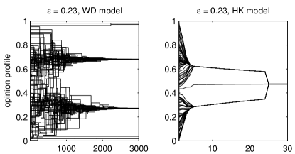
Figure 1: Example processes for the WD and HK model. With initial profile of 100 agents with random equally distributed opinions within $[0,1]$.

Figure 1 shows example processes for both models. In both models the processes converge to a stabilized opinion profile, where opinions have divided into a certain number of clusters. The stabilization can be proved analytically, even for a bigger class of models [8]. The dynamical behavior can be described in the same way: The contractive force of compromising brings opinions together, but bounded confidence forces the agents to form clusters where higher local agent densities occur, thus confidence to other agents gets lost.

We will briefly summarize the known results, which we consider in this paper. At first, results about the WD model. The number of expected major clusters is roughly the integer part of $1/2\varepsilon$ [1]. But not all agents join the major clusters, some remain outliers or form minor clusters (like in figure 1 at the extremes).

In the HK model there are slightly lower numbers of expected clusters as in the WD model, for details see [9]. Convergence to consensus may take very long, due to very few agents remaining in the middle and attracting all other agents very slowly (like in figure 1 but it can be more drastic for larger $n$).

Both models were extended in several ways. The WD model to relative agreement, smooth bounded confidence, dynamics on small world networks [10], heterogeneous bounds of confidence, dynamics of the bounds of confidence and vector opinions [1]. Special starting distributions were used to model a drift to the extremes [2]. The HK model has been extended to asymmetric [3] or heterogeneous bounds of confidence [11], multidimensional opinions [12]. Some further proposals are in [13].

We show some statistical simulation results in figure 2 to give a chance to look into more details. For the graphic of added stabilized profiles we divided the opinion interval $[0,1]$ into 25 subintervals of equal size and count the number of agents in each subinterval. In the graphic at the bottom left dotted lines represent frequencies of 1 cluster and 2 clusters where we count only clusters with more then 5 agents, thus outliers and minor clusters are ignored.

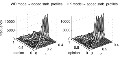
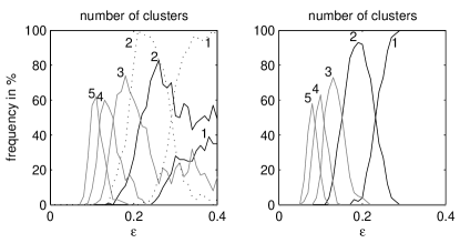
Figure 2: Added stabilized profiles (top), frequencies of the number of evolving clusters (bottom) for the WD (left hand) and the HK (right hand) model. Basic data: 100 initial profiles with 200 agents and random opinions between 0 and 1; Graphics data: stabilized profiles computed for $\varepsilon=0,\stackrel{{\scriptstyle+0.01}}{{\dots}},0.4$. (Dotted lines: without minor clusters.)

The number of agents $n$ is a parameter which is not much studied due to computing time problems. One idea of the following analysis studies with interactive Markov chains is to get a feeling about the dynamics we will approach with greater $n$.

3 Interactive Markov Chains

In this section we want to reformulate the models of WD and HK as interactive Markov chains. Thus, we switch from $n$ agents to an idealized infinite population, which we divide into $n$ classes of opinions. Instead of an opinion profile $x(t)\in\mathbb{R}^{n}$ we consider a discrete opinion distribution $p(t)\in S^{n}:=\{p\in[0,1]^{1\times n}$ with $\sum_{i=1}^{n}p_{i}=1\}$ as the state of our system at time $t\in\mathbb{N}$. $S^{n}$ is the $(n-1)$-dimensional unit simplex of row vectors. A discrete opinion distribution is a row vector while the opinion profile is a column vector. For convenience we define $p_{i}=0$ for all $i\not\in\underline{n}$.

We will define transition probabilities $b_{ij}(p)\in[0,1]$ for agents in class $i$ to go to class $j$. For all $i\in\underline{n}$ should hold $\sum_{j=1}^{n}b_{ij}(p)=1$. Thus the transition matrix $B(p)=[b_{ij}(p)]$ is row-stochastic. The interactive Markov chain for an initial opinion distribution $p(0)$ is the sequence of opinion distributions $(p(t))_{t\in\mathbb{N}_{0}}$ recursivly defined through

$$p(t+1)=p(t)B(p(t)).$$ (2)

This Markov chain is called interactive (according to Conlisk [14]) because the transition matrix depends on the state of the system in the actual time step.

In analogy to the bound of confidence $\varepsilon$ we define a discrete bound of confidence $k\in\mathbb{N}$, which defines that the transitions of opinions of class $i$ can only be influenced by opinions of the classes ${i-k,\dots,i+k}$.

If we imagine that the opinions $1,\dots,n$ are representatives for an equidistant partition of the interval $[0,1]$ in the way $i\leftrightarrow[\frac{i-1}{n},\frac{i}{n}]$, we draw a heuristic analogy $\frac{k}{n}\leftrightarrow\varepsilon$. Thus, if we go $k,n\to\infty$ with $\frac{k}{n}\to\varepsilon$ we can ’converge’ to an agent-based model with $\infty$ agents, opinions in $[0,1]$ and bound of confidence $\varepsilon$.

In this setting we may consider $n$ as a parameter how accurate a continuous opinion can be communicated, e.g. how many steps do we allow on the continuous scale from minimum to maximum opinion. (The topic of accuracy is discussed for agent-based models in [15] in the context of opinion versus attitude dynamics.)

Calculation of the interactive Markov chains will be interesting regarding the following questions.

1. Does the Markov chain produce the same dynamical behavior as the agent-based models?

2. What conclusions can be drawn from the results about the idealized infinite populations in the Markov Chains to the finite cases of agent-based systems?

3. What is the effect of the accuracy of the Markov chains $n$?

We will start with the definiton of the WD Markov chain.

Definition 3.1 (interactive WD Markov chain).

We define the WD transition matrix for an opinion distribution $p\in S^{n}$ and a discrete bound of confidence $k\in\mathbb{N}$ as

$$b_{ij}(p,k):=\left\{\begin{array}[]{ll}\frac{\pi^{i}_{2j-i-1}}{2}+\pi^{i}_{2j-i}+\frac{\pi^{i}_{2j-i+1}}{2},&\hbox{if $i\neq j$, }\\ q_{i},&\hbox{if $i=j$.}\\ \end{array}\right.$$

with $q_{i}=1-\sum_{j\neq i,j=1}^{n}b(p,k)_{ij}$ and

$$\pi^{i}_{l}:=\left\{\begin{array}[]{ll}p_{l},&\hbox{if $|i-l|\leq k$}\\ 0,&\hbox{otherwise}\\ \end{array}\right.$$

(Attention $i$ in $\pi^{i}$ is another index not an exponent!) Let $p(0)\in S^{n}$ be an initial opinion distribution. The Markov chain (2) with WD transition matrix is called interactive WD Markov chain with discrete bound of confidence $k$.

Remember that we defined $p_{i}=0$ for all $i\not\in\underline{n}$. By the founding idea of the WD model an agent with opinion $i$ moves to the new opinion $j$ if he compromises with an agent with opinion $i+2(j-i)=2j-i$. The probability to communicate with an agent with opinion $2j-i$ is of course $p_{2j-i}$. Thus, the heuristic of random pairwise interaction is represented. The terms $\frac{\pi^{i}_{2j-i-1}}{2},\frac{\pi^{i}_{2j-i+1}}{2}$ stand for the case when agents with opinion $i$ communicate with agents with opinion $l$, but the distance $|i-l|$ is odd. In this case the population should go with probability $\frac{1}{2}$ to one of the two possible opinion classes $\lfloor\frac{i+l}{2}\rfloor,\lceil\frac{i+l}{2}\rceil$.

(This definition is inspired by the rate equation in [16]. But they used continuous time. Further on we introduced the discrete bound of confidence.)

The interactive Markov chain for the HK model looks as follows.

Definition 3.2 (interactive HK Markov chain).

Let $p\in S^{n}$ be an opinion distribution and $k\in\mathbb{N}$ be a discrete bound of confidence. The $k$-local mean of $p$ at $i\in\underline{n}$ is

$$M_{i}(p,k):=\frac{\sum\limits_{m\in\underline{n},|i-m|\leq k}mp_{m}}{\sum\limits_{m\in\underline{n},|i-m|\leq k}p_{m}}.$$

We define (with abbreviation $M_{i}:=M_{i}(p,k)$ the HK transition matrix) as

$$b_{ij}(p,k):=\left\{\begin{array}[]{ll}1&\hbox{if $j=M_{i}$,}\\ \lceil M_{i}\rceil-M_{i}&\hbox{if $j=\lfloor M_{i}\rfloor$, $j\neq M_{i}$,}\\ M_{i}-\lfloor M_{i}\rfloor&\hbox{if $j=\lceil M_{i}\rceil$, $j\neq M_{i}$,}\\ 0&\hbox{otherwise.}\\ \end{array}\right.$$

Let $p(0)\in S^{n}$ be an initial opinion distribution. The Markov chain (2) with HK transition matrix is called interactive HK Markov chain with discrete bound of confidence $k$.

Each row of the HK transition matrix $B(p,k)$ contains only one or two adjacent positive entries. The population with opinion $i$ goes completely to the $k$-local mean opinion if this is an integer. Otherwise they distribute to the two adjacent opinions. The fraction which goes to the lower (upper) opinion class depends on how close the $k$-local mean lies to it. Thus, the heuristic of overall averaging in a local area is represented here.

For both interactive Markov chains we define a stabilized distribution $p^{\ast}\in S^{n}$ as a fixed point (that means that it holds $p^{\ast}=p^{\ast}B(p^{\ast})$). Both models converge to stabilized distributions for every initial distribution, while the set of possible stabilized distributions is huge. This properties are stated by observation of example Markov processes. There is no formal proof at this time.

In a first analysis step we will focus on the initial distribution $p(0)\in S^{n}$ which is equally distributed $p_{1}=\dots=p_{n}=\frac{1}{n}$. This coincides with the agent-based model if we start with $x\in[0,1]^{n}$ where the $x_{i}$ are chosen at random and equally distributed.

Figure 3 shows processes for both models with $n=101,k=9$ (coincides with $\varepsilon\approx 0.089$) at characteristic time steps. We see clustering dynamics as in the agent-based models. Five major clusters emerging in the WD model and three major clusters emerging in the HK model.

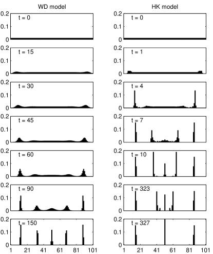
Figure 3: WD and HK process for equally distributed initial distribution with $n=101,k=9$ at characteristic time steps.

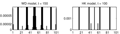
Figure 4: Same processes as in figure 3 with finer $y$-scale at certain time steps to show minor clusters after stabilization for WD and minor clusters attracting major clusters for HK.

The finer scaled plots in figure 4 give more insights. It shows for the WD model four minor clusters in the stabilized distribution. (The distribution at $t=150$ is not totally stabilized, but very close to the distribution it converges to. E. g. the big central cluster that we see in the blow-up figure 4 will converge slowly to a one bin cluster. The first two off-central clusters will converge each to a two bin cluster as we see it already in figure 3.) We got minor clusters at both extremes and two minor clusters between major clusters, which will survive forever. The minor clusters are only visible in the blow-up figure. There are no minor clusters between the central and his adjacent major clusters.

For the HK model we see the possibility of very slow convergence in the HK model on the right side in figure 3, which can be explained by figure 4. There we see two small clusters which hold contact between the central cluster and the both adjacent major clusters. The dynamic reaches a stabilized distribution with three major clusters at $t=327$. We call the states from $t=10$ to $t=326$ ’meta-stable’ because they look like stable.

Thus, both special features that we mentioned for the agent-based models (minor clusters for WD model and very slow convergence in HK model) also occur in the aggregated models of the interactive Markov chains. This effects may be seen as artifacts by simulators but they should be regarded as intrinsic to the dynamic’s behavior (at least for great numbers of agents).

To get a complete overview about the random equally distributed initial distribution we will calculate a ’discrete’ bifurcation diagram for both models. We will calculate the stabilized distributions for all processes for $n=1001$ and $k=50,\stackrel{{\scriptstyle+1}}{{\dots}},300$ (thus $\varepsilon\approx 0.05,\dots,0.3$). Our bifurcation diagram is called ’discrete’ because the analyzed bifurcation parameter $k$ is discrete, which does not fit into the usual terms of bifurcation theory. In our setting a bifurcation is an abrupt change in the stabilized profile in one discrete step of the parameter $k$.

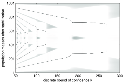
Figure 5: Bifurcation diagram for the WD model. $n=1001,k=50,\dots,300$.

Figure 5 and 6 show discrete bifurcation diagrams for the interactive WD and HK Markov chains. The gray scale symbolizes the masses at the specific positions: White is zeros, black is fair above zero and grey is slightly above zero. We see the major clusters as black lines. (Notice that a fully converged cluster normally consists of two adjacent non-zero entries in $p$ surrounded by zero entries. You can not see this in the figure.)

We describe the bifurcation diagram for the WD process. At first we have to notice again that the diagram is not fully converged due to computation time. Going further on in time the gray areas would converge slowly to gray lines of minor clusters. Going form $k=300$ down to 50 we see at first one central cluster and minor clusters at the extremes (that will converge to the total extremes), then the central cluster bifurcates into two major clusters at roughly $k\approx 270$, then a small central cluster nucleates ($k\approx 220$), the new central cluster is growing and the two former clusters drift away from the center. At $k\approx 150$ two minor clusters emerge. At roughly 125 the central cluster bifurcates again into two clusters, while the minor clusters vanish for a short phase. The same bifurcation and nucleation procedure repeats on a shorter $k$-scale from 125 to 80 and so on.

The existence or absence of minor clusters between major clusters can be explained with the accuracy $n$. Only if the accuracy leaves enough classes between two major clusters a minor cluster can survive in between.

A similar bifurcation diagram for the differential equation describing the same heuristics is in [16].

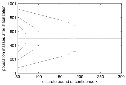
Figure 6: Bifurcation diagram for the HK model. $n=1001,k=50,\dots,300$.

In figure 6 we see the bifurcation diagram for the HK model. In contrast to the WD diagram the processes in this diagram have converged completely. Going form $k=300$ down to 50 we see one central cluster, then at $k=190$ a bifurcation into two major clusters occurs while very little mass remains in a central cluster. Then (k=175) we get into an interesting phase where consensus strikes back, but not for all $k$, sometimes we end up in three clusters. The outer clusters begin to drift outwards away from their old position. Consensus in this $k$-phase happens due to very slow convergence to the center like in figure 3. The last consensus appears at $k=153$ (where convergence lasts 21424 time steps). Then the existence of the two outer clusters and their outward drift is stable until the central cluster bifurcates again on a shorter time scale (two major clusters $k=100,99,98$, consensus strikes back $k=97,\dots,89$, then stable 5 clusters) and so on. Remarkably is that we reach a consensus at the HK Markov chain for $\varepsilon=k/n>0.19$ but in the tested agent-based model (figure 2) with 200 agents the chance for consensus is only for $\varepsilon\geq 0.23$ fair.

The interactive Markov chains raises the question: Is it important to have an even or odd number of opinion classes? In other words, is it important to have a central opinion class? The impact of the existence of a central opinion class is very high for the HK model as we see in figure 7. For the WD model the bifurcation diagram for $n=1000$ looks just as figure 5.

Figure 7: Bifurcation diagram for the HK model. $n=1000,k=50,\dots,300$.

There are two differences between the HK bifurcation diagrams in figures 6 and 7 which are generic for other other pairs $n,n+1$. First, the bifurcation from consensus to polarization occurs earlier for even $n$ (at $k=200$) and the central clusters disappears totally at that bifurcation and nucleates again some $k$-steps later. Second the ’consensus strikes back’ $k$-phase changes into a polarization phase, but with major clusters closer to the center. As for $n=1001$ this is not stable in that $k$-phase, for some values we reach two outer majors and a central cluster.

Both phenomena can be explained through the meta-stable state that we reach after the first time steps (in figure 3 at $t=10$). For an odd number of opinion classes we have a central cluster consisting of only one opinion class, while for an even number of opinion classes the central cluster contains two opinion classes.

4 Conclusion

We summarize. The basic dynamical feature of both models is: Stabilization to a fixed point and fixed points are opinion distributions where the mass clusters in pairs of adjacent classes which have distances greater than $k$ to all other pairs. This coincides with the agent-based models (neglecting the clustering in pairs of opinion classes). The differences in the agent based models (number of clusters at specific $\varepsilon$, existence of outliers) appear also and even more drastic in the Markov chain models. We show that two properties which may be seen as artifacts are intrinsic to the dynamical behavior.

The WD model leads for equally distributed initial distributions to major clusters which lie as far from each other, that it is possible for small cluster to survive between them, but only for great $n$ and not too low $k$. The existence of minor clusters depends also on $\frac{k}{n}$.

The HK model leads to major clusters only (except the central cluster, which may be small). In the center we can reach a meta-stable state with two major clusters, a central cluster and between major and central cluster small clusters, which attract the big ones very slowly to the center. An even number of opinions lowers the chances for central consensus because the central mass can split.

In future research we should ask how robust the results are with other initial distributions. A first but not systematic calculation leads to the hypothesis that the basic features (clustering in pairs, space for minor clusters for WD and meta stable states with long convergence for HK) also characterize the dynamics for other initial distributions. Further on stabilization should be proved.

The heuristics of these opinion dynamic models is not based on quantitative data. Thus, they can not predict quantitative opinion clustering. Conclusions about real opinion dynamics should be drawn in a qualitative manner that links the heuristics of the model to the dynamical outcome, in a way like: Bounded confidence in opinion dynamics about ’continuous’ topics leads to clustering. Pairwise communication produces minorities while averaging over all acceptable opinions may lead to meta-stable situations where consensus is possible but reaching it will take very long.

Acknowledgment

The author thanks the Friedrich-Ebert-Stiftung, Bonn, Germany for financial funding.

References

- [1] Gérard Weisbuch, Guillaume Deffuant, Frédéric Amblard, and Jean-Pierre Nadal. Meet, Discuss and Segregate! Complexity, 7(3):55–63, 2002.
- [2] G. Deffuant, D. Neau, F. Amblard, and G. Weisbuch. How can extremism prevail? A study based on the relative agreement interaction model. Journal of Artificial Societies and Social Simulation, 5(4), 2002. www.soc.surrey.ac.uk/JASSS/5/4/1.html.
- [3] Rainer Hegselmann and Ulrich Krause. Opinion dynamics and bounded confidence, Models, Analysis and Simulation. Journal of Artificial Societies and Social Simulation, 5(3), 2002. www.soc.surrey.ac.uk/JASSS/5/3/2.html.
- [4] M. H. DeGroot. Reaching a consensus. Journal of American Statistical Association, 69(345):118–121, 1974.
- [5] Samprit Chatterjee and Eugene Seneta. Towards consensus: Some convergence theorems on repeated averaging. J. Appl. Prob., 14:159–164, 1977.
- [6] Noah E. Friedkin and Eugene C. Johnson. Social influence and opinion. Journal of Mathematical Sociology, 15(3-4):193–205, 1990.
- [7] Andreas Flache. When will they ever make up their minds? The social structure of unstable decision making. Journal of Mathematical Sociology, 28:171–196, 2004.
- [8] Jan Lorenz. A stabilization theorem for dynamics of continuous opinions. Physica A, to appear 2005.
- [9] Diemo Urbig and Jan Lorenz. Communication regimes in opinion dynamics: Changing the number of communicating agents. In Proceedings of the Second Conference of the European Social Simulation Association (ESSA), September 2004.
- [10] F. Amblard and G. Deffuant. The role of network topology on extremism propagation with the relative agreement opinion dynamics. Physica A, 343:725–738, 2004.
- [11] Jan Lorenz. Opinion dynamics with different confidence bounds for the agents. Workshop on Economics of Heterogeneous Interacting Agents, WEHIA Kiel, May 2003. find it at www.janlo.de.
- [12] Jan Lorenz. Mehrdimensionale Meinungsdynamik bei wechselndem Vertrauen. Master’s thesis, University of Bremen, 2003. Find it at www.janlo.de.
- [13] R. Hegselmann. Laws and Models in Science, chapter Opinion dynamics: Insights by radically simplifying models, page 1 29. 2004.
- [14] John Conlisk. Interactive Markov Chains. Journal of Mathematical Sociology, 4:157–185, 1976.
- [15] Diemo Urbig. Attitude dynamics with limited verbalisation capabilities. Journal of Artificial Societies and Social Simulation, 6(1), 2003. www.soc.surrey.ac.uk/JASSS/6/1/2.html.
- [16] E. Ben-Naim, S. Redner, and P.L. Krapivsky. Bifurcation and patterns in compromise processes. Physica D, 183:190–204, 2003.