3D ${\cal N}{=}1$ SYM Chern-Simons theory on the Lattice

Abstract

We present a method to implement 3-dimensional ${\cal N}{=}1$ SUSY Yang-Mills theory (a theory with two real supercharges containing gauge fields and an adjoint Majorana fermion) on the lattice, including a way to implement the Chern-Simons term present in this theory. At nonzero Chern-Simons number our implementation suffers from a sign problem which will make the numerical effort grow exponentially with volume. We also show that the theory with vanishing Chern-Simons number is anomalous; its partition function identically vanishes.

I Introduction

Lattice studies of supersymmetric field theories have long been an elusive goal. The lattice regularization generally breaks the supersymmetry and the IR limit of the lattice theory typically contains SUSY breaking fermion and scalar mass terms, which in 4 dimensions arise at all orders in perturbation theory. Much effort has recently been directed toward finding ways to avoid these terms by creative choices of lattice actions and/or generalized supersymmetry algebras Kaplan_lattsusy ; Catterall2d .

One way around this problem is to consider minimally supersymmetric Yang-Mills theory, which contains only gauge fields and fermions. The theory is then automatically (accidentally) supersymmetric provided one can correctly implement the fermions. Recent advances in fermion implementations Kaplan_domainwall ; Narayanan have made it possible to achieve this program in 4 dimensions 4DSUSY .

In this paper we instead consider 3-dimensional minimally supersymmetric Yang-Mills theory ($N{=}1$ supersymmetry, with two real supercharges). This theory is free of scalars and so correct implementation of the fermions again yields the right supersymmetric IR limit “accidentally.” However, the implementation of the fermions is quite intricate, since one must impose a Majorana condition, and the implementation is further complicated by phases arising both from the fermionic determinant and from a Chern-Simons (CS) term, which is possible (and we will show, required) in this theory.

The goal of this paper is to give a recipe for studying $N{=}1$ SUSY in three dimensions with a Chern-Simons term on the lattice. This theory is believed to display very interesting nonperturbative properties that make it a prime target for simulation. In particular, Witten has conjectured Witten3d that the theory either preserves or spontaneously breaks supersymmetry, depending on the value of the Chern-Simons term. A lattice study of the theory would then constitute the first test (to our knowledge) of a nonperturbative supersymmetry breaking mechanism.

The paper will be organized as follows. In section II we will review the continuum action of the theory, the necessity of a Chern-Simons term, and the anomaly condition which fixes the Chern-Simons term to take certain half-integer values. We will also present a proof, apparently unrecognized before, that the theory with vanishing Chern-Simons term has a vanishing partition function and is therefore not well defined. In section III we will describe the discretization process, showing that the magnitude of the fermion determinant can be included using a rooted 3-D (2 component) Wilson-Dirac fermion with SW improvement and mass counterterm. We then show how to extract the Chern-Simons phase and the phase of the properly regularized rooted determinant. We leave the simulation itself for a future work; the goal here is to show that such simulations can be done and to provide the required tools.

II 3D $N{=}1$ SYM in the Continuum

The field content of the theory consists of a gauge field and a 2-component, Majorana fermion in the adjoint representation (gaugino). In 4-dimensional notation, the gaugino is a 2-component Weyl fermion which has been further reduced from 2 complex to 2 real components by the application of a Majorana condition (possible in 3 dimensions). The Euclidean action is

$$S=\frac{1}{g^{2}}\int d^{3}x\Bigg{(}\frac{1}{4}F^{a}_{\mu\nu}F^{a}_{\mu\nu}+\frac{1}{2}\bar{\psi}_{a}(\hbox to0.0pt{\hbox to8.55695pt{\hfil/\hfil}\hss}D\psi)_{a}\Bigg{)}\,.$$ (1)

With these conventions the eigenvalues of the Dirac operator are all pure imaginary. Because the fermion is in a real representation of the gauge group, the fermionic operator possesses a doubled spectrum; if $\psi_{\lambda}$ is an eigenvector of $\hbox to0.0pt{\hbox to8.55695pt{\hfil/\hfil}\hss}D$ with eigenvalue $i\lambda$, then $\epsilon\psi_{\lambda}^{*}$ (where $\epsilon=-i\sigma_{2}$) is also an eigenvector with the same eigenvalue;

$$\sigma_{\mu}D_{\mu}\psi_{\lambda} = i\lambda\psi_{\lambda}$$

$$\sigma_{\mu}^{*}D_{\mu}\psi^{*}_{\lambda} = -i\lambda\psi^{*}_{\lambda}$$

$$\epsilon\sigma_{\mu}^{*}D_{\mu}\psi^{*}_{\lambda} = -i\epsilon\lambda\psi^{*}_{\lambda}$$

$$\sigma_{\mu}D_{\mu}(\epsilon\psi^{*}_{\lambda}) = i\lambda(\epsilon\psi^{*}_{\lambda})\,.$$ (2)

The Majorana condition consists of taking only one of these degenerate sets of eigenvalues to define the fermion contribution to the path integral. That is, in the path integral replace

$$\det\hbox to0.0pt{\hbox to8.55695pt{\hfil/\hfil}\hss}D=\prod_{i}\lambda_{i}\quad\to\quad\sqrt{\det\hbox to0.0pt{\hbox to8.55695pt{\hfil/\hfil}\hss}D}=\prod_{i}\!^{\prime}\,\lambda_{i}$$ (3)

where $\prod_{i}\!^{\prime}\,$ is defined by taking only one eigenvalue from each degenerate pair.

We can add a Chern-Simons term to this action in 3D provided we include an appropriate mass term for the fermions so that SUSY is retained:

$$S_{CS} = -\frac{ik}{16\pi}\int_{x}\epsilon_{\mu\nu\rho}\bigg{(}F^{a}_{\mu\nu}A^{a}_{\rho}-\frac{1}{3}f_{abc}A^{a}_{\mu}A^{b}_{\nu}A^{c}_{\rho}\bigg{)}+\frac{1}{2}\frac{k}{4\pi}\int_{x}\bar{\psi}_{a}\psi_{a}$$

$$\equiv -2\pi ikN_{cs}+\frac{1}{2}\frac{m}{g^{2}}\int_{x}\bar{\psi}\psi\,,\qquad m=\frac{g^{2}k}{4\pi}\,.$$

Here $k$ is the level of the CS theory or CS coupling. It is straightforward to check that the action is indeed invariant under the SUSY transformations

$$\delta A^{a}_{\mu}=\bar{\alpha}\sigma_{\mu}\psi_{a}\,,\quad\delta F^{a}_{\mu\nu}=\bar{\alpha}(\sigma_{\nu}\partial_{\mu}-\sigma_{\mu}\partial_{\nu})\psi_{a}$$

and $$\delta\psi_{a}=-\frac{i}{2}\epsilon_{\mu\nu\rho}F^{a}_{\mu\nu}\sigma_{\rho}\alpha\,,$$ (5)

with $\alpha$ the Grassman valued Majorana spinor parameterizing the SUSY transformation. Our convention for Majorana spinors is $\bar{s}=s^{\top}\epsilon$.

It has long been known Redlich:1983dv ; Witten3d that - for gauge group SU($N_{\rm c}$) - $k$ must equal $N_{\rm c}/2$ modulo an integer to avoid a gauge anomaly so that, in particular, the theory with odd $N_{\rm c}$ is ill defined for vanishing CS term. In Sec. II.1 we review this argument and present a similarly motivated argument for the theory with even $N_{\rm c}$ that implies that these theories are also ill defined for vanishing $k$.

II.1 Anomalies in 3D SU($N_{\rm c}$) SYM

In Wittensu2:1982 Witten gave the first example of a theory with a rooted determinant that is sick with a global gauge anomaly, namely 4D SU(2) gauge theory with an odd number of left-handed fermion doublets. The problem with this theory is that it is impossible to define the fermionic determinant over the space of gauge connections (gauge fields modulo all gauge transformations) such that it is both continuous and single-valued.

We will review the 3D analog, formulated by Redlich Redlich:1983dv for gauge group SU($N_{\rm c}$), which is slightly simpler and is of immediate importance for the current discussion. The general issue is that there are phase ambiguities in performing Grassman integrations. This is a problem in writing a path integral unless the phase ambiguity can be reduced to a single gauge-field independent phase, which factors out from the partition function and cancels in determining any correlation function. Therefore we pick some gauge field $A_{0}$, (chosen so that the Dirac operator has no zero eigenvalues) and call its contribution to the path integral real and positive. Then we determine the sign for any other configuration $A$ by insisting on continuity of $\det\hbox to0.0pt{\hbox to8.55695pt{\hfil/\hfil}\hss}D$ along a path from $A_{0}$ to $A$. This is possible for any gauge field because our group manifold is path connected.

The procedure is sketched in Fig. 1: we watch the low lying eigenvalues of the spectrum as the path parameter $t$ is varied from $0$ to $1$ and count the number of eigenvalue pairs that change sign from positive to negative. This gives the relative sign of the two determinants in the path integral.

$\begin{array}[]{c@{\hspace{.6in}}c}\epsfbox{interpolate.eps}\hfil\hskip 43.36243pt&\epsfbox{spectral_flow.eps}\end{array}$

Figure 1: A path in configuration space and its associated eigenvalue flow

This prescription is unique unless the number of eigenvalue zero-crossings depends on the path. This can happen because the space of connections is multiply connected; if two paths from $A_{0}$ to $A$ form a noncontractible loop, there is no guarantee that they lead to the same sign choice for $\det\hbox to0.0pt{\hbox to8.55695pt{\hfil/\hfil}\hss}D(A)$.

Call the space of 3D gauge connections $X$. It contains noncontractible loops if the third homotopy group $\pi^{3}$ of the gauge group is nontrivial. (It is the third homotopy group because we are in 3 dimensions.) This is the case for all SU($N_{\rm c}$), for which $\pi^{3}={\cal Z}$. Consider a nontrivial loop from $A_{0}$ back to $A_{0}$.

Figure 2: A closed loop in configuration space with a non-trivial winding number

This path is effectively a 4D gauge field configuration, where the space is $S_{1}\times$ 3D space and the 4D gauge fields are $A_{M}=(A^{\mu},A_{4}=0)$. The path is noncontractible if the instanton number of this gauge field configuration is nonzero. The four dimensional Weyl determinant has a number of zero modes determined by the Atiyah-Singer theorem Atiyah-Singer ; for the fundamental representation this is 1 and for the adjoint representation this is $2N_{\rm c}$. The 4D zeros correspond to zero crossings, and therefore sign flips, of the 3D fermionic determinant. If the number of sign flips in traversing the loop is odd, then the definition of the determinant cannot be both continuous, nontrivial, and single valued.

For our case this is relevant because we want the square root of the Weyl determinant; the $2N_{\rm c}$ zero crossings become $N_{\rm c}$ zero crossings when we choose one from each pair of eigenvalues, and this leads to a sign flip if $N_{\rm c}$ is odd.

There is an additional sign if the theory is defined with a nonzero Chern-Simons term. The CS term picks up a factor of $2\pi\nu$ in traversing a path of instanton number $\nu$, so the path integral picks up an overall factor of

$$(-1)^{\nu N_{\rm c}}\exp(i2\pi\nu k)\,.$$ (6)

This implies that, in order to avoid a gauge anomaly, $k{=}N_{\rm c}/2$ modulo an integer. Only certain (half-integer) values of the Chern-Simons term are allowed, and in particular, the theory with $N_{\rm c}$ odd and vanishing CS term is ill defined.

We will now show that the supersymmetric theory with $N_{\rm c}$ even and Chern-Simons coefficient $k=0$ (and therefore fermion mass of zero) is also anomalous, a point which to our knowledge has not been noticed before. Consider a configuration ${A(x)}$ and its parity dual ${A^{\prime}(x)=-A(-x)}$. We claim that these give canceling contributions to the partition function if the Chern-Simons term is absent and the fermion mass is zero. They clearly have the same bosonic action, so we must show only that their rooted fermion determinants are equal and opposite. We define the sign of the rooted determinant for configuration ${A(x)}$ to be positive and connect them with a path from ${A(x)}$ to the trivial vacuum and from the trivial vacuum to ${A^{\prime}(x)}$ via the parity dual of this path (see again Fig. 1).

The Dirac operator for the trivial vacuum configuration has $(N_{\rm c}^{2}-1)$ pairs of zero eigenvalues (we implicitly work on a torus with standard boundary conditions). There are then $(N_{\rm c}^{2}-1)$ pairs of eigenvalues that cross zero at the vacuum configuration. Furthermore, if $n_{+}$ pairs cross zero somewhere on the path between ${A(x)}$ and the vacuum, than the number of pairs $n_{-}$ that cross zero between the vacuum and ${A^{\prime}(x)}$ will be the same. The total number of pairs which change sign in going from ${A(x)}$ to ${A^{\prime}(x)}$ is therefore $(N_{\rm c}^{2}-1)+2n_{+}$. This is odd, so the fermion rooted determinant flips sign and the configurations give canceling contributions to the partition function, which vanishes identically. An example of the eigenvalue flow for gauge group SU($2$) is shown in Fig. 3 for the case $m{=}0$.

This problem is avoided at nonzero Chern-Simons term because ${A(x)}$ and ${A^{\prime}(x)}$ have opposite Chern-Simons number and so enter the partition function with opposite phase, rather than canceling. Similarly, at nonzero fermion mass the eigenvalues of the Dirac operator are complex and introduce nonzero phases which are opposite between the configuration and its parity dual.

Figure 3: Flow of almost zero mode eigenvalues of the Dirac operator as the configuration is varied between parity conjugate gauge fields on a path through the vacuum.

II.2 Regularization dependence of determinant

Figure 4: Eigenvalues for 20 Wilson fermion configurations in a $8^{3}$ box at $g^{2}a=0.5$, illustrating the “return loops” in the complex plane.

It is necessary to clarify what is meant by the “continuum” fermionic determinant. The issue is that continuum theories are always defined as limits of discrete (or otherwise regularized) theories and in a discrete theory with volume regularization there are a finite number of eigenvalues for the Dirac equation. In traversing a closed loop with nonzero instanton number, we just saw that a nonzero number of eigenvalues cross from negative to positive value. Since the final configuration is the same as the starting one, it has the same spectrum. Since there are a finite number of negative eigenvalues, there must be some compensating flow of positive eigenvalues to negative, somewhere in the complex plane. In other words, eigenvalues must “return” somewhere in the complex plane. We illustrate this for Wilson fermions in Fig. 4. The figure superimposes the eigenvalue spectra, in the complex plane, of 20 quenched gauge field configurations in an $8^{3}$ box with lattice spacing $g^{2}a=0.5$. Each dot is a pair of eigenvalues (the pairing of the spectrum discussed in the last section occurs for both the Wilson and overlap lattice implementations of the Dirac operator). The spectrum of eigenvalues for $\hbox to0.0pt{\hbox to8.55695pt{\hfil/\hfil}\hss}D$ parallels the imaginary axis near zero but bends out into the complex plane for large eigenvalues $\lambda\sim 1/a$ and forms a loop, so eigenvalues moving from negative to positive values “push” eigenvalues around the loop to reappear at negative values. These extra vanishing-imaginary-part eigenvalues are the lattice fermion doublers which have been pushed out into the complex plane by the Wilson term; for the Wilson action in 3 dimensions there are actually 3 extra places where eigenvalues cross zero imaginary part, corresponding to $(\pi,0,0)$, $(\pi,\pi,0)$, and $(\pi,\pi\,\pi)$ type doublers.

The problem is that this “return loop” will contribute to the partition function even in the continuum limit. Because it represents deeply UV physics, its contribution to the partition function must be representable in an effective IR description in terms of local effective operators. The 3D theory has only one marginal operator, which is the Chern-Simons term. Therefore the return loop can (and will) induce a Chern-Simons term, but will not otherwise change the infrared description (in the small $a$ limit). It is easy to see that the size of this Chern-Simons term is fixed by the rate of spectral flow near zero; the number of eigenvalues which circle around the loop must be the number needed to refill the negative eigenvalues when the spectrum flows upwards. The sign of this extra Chern-Simons term depends on whether the return loop is at positive or negative imaginary part, which is a regularization detail. The desired continuum theory is the one in which this regularization effect has been removed by a Chern-Simons number counterterm.

III The Discretization

This section describes the discretization of $N{=}1$ SYM with a Chern-Simons term in 3D. The theory contains nontrivial phases; that is, different gauge field configurations contribute to the partition function with different complex phase as well as different magnitude. The plan is to treat this using the Edinburgh method; one studies the theory on the lattice by building a Markov chain sample weighted by the magnitude of the action $|\exp(-S)\sqrt{\det\hbox to0.0pt{\hbox to8.55695pt{\hfil/\hfil}\hss}D}|$ and then includes the phase as part of the observable. Phase cancellation reduces the statistical power in a volume dependent way. Therefore our implementation is on the same footing as finite chemical potential simulations in QCD; they work in principle, but whether they work in practice depends on how severe the phase cancellation problem turns out to be.

The implementation consists of two parts; the real part of the bosonic action and magnitude of the fermionic determinant, and the phase. The real bosonic action is completely standard. We describe the magnitude of the determinant first, then the Chern-Simons part of the phase, then the phase in the determinant.

III.1 Fermion Implementation

Though there may be some advantages to using an overlap fermion implementation to do the simulation, we believe that the numerical simplicity of the Wilson implementation makes it a much more sensible choice. The usual problems with Wilson fermions are less severe than in 4 dimensions; chiral symmetry is a non-issue because there is no such thing in 3 dimensions, and the additive renormalization of the mass is well behaved because the theory is super-renormalizable. One can easily work at a fine lattice spacing where the problem of exceptional configurations is well under control (note that we are only interested in the theory at finite fermion mass, since as we just argued the massless theory is anomalous).

The fermionic action reads

$$S_{W} = a^{3}\sum_{x}\bar{\psi}_{x}\left(m_{0}+\frac{3r}{a}\right)\psi_{x}$$ (7)

$$-a^{3}\sum_{x,\,\mu}\bar{\psi}_{x}\frac{(r-\sigma_{\mu})U_{\mu}(x)\psi_{x}+(r+\sigma_{\mu})U^{\dagger}_{\mu}(x{-}\mu)\psi_{x{-}\mu}}{2a}\,.$$

We can improve the convergence of the spectrum to the continuum limit from $O(a)$ to $O(a^{2})$ via the 3D analog of the Sheikholeslami-Wohlert term Sheikholeslami:1985ij (SW) term

$$S_{sw}=a^{3}\sum_{x,\,\mu,\,\nu}\frac{rc_{sw}}{16}\bar{\psi}_{x}[\sigma_{\mu},\sigma_{\nu}]\bigg{(}P_{\mu\nu}(x)-P^{\dagger}_{\mu\nu}(x)\bigg{)}\psi_{x}$$ (8)

Here $P_{\mu\nu}(x)$ is the average of the 4 plaquettes in the $\mu\nu$ plane as shown in Fig. 5. This improvement is probably necessary to implement simulations at reasonable lattice spacings.

Figure 5: Clover field strength for the Sheikholeslami-Wohlert improvement term.

Since the 3D theory is superrenormalizable we need only the tree level determination of the SW coefficient, $c_{sw}{=}1$, to remove $O(a)$ corrections other than mass renormalizations. Much of the complication of the improvement in 4D is thus avoided in the 3D version.

The improvement to the spectral properties is quite dramatic, though it parallels closely the improvement in 4D so we refer the interested reader to, for example, Gattringer:1998ab for analysis of 4D Dirac operator spectra with improved and unimproved actions in a situation which is fairly analogous to the cases we consider in 3D. Fig. 6 shows an example of the improvement to the physical branch of the spectrum for 20 configurations on a $14^{3}$ lattice with $g^{2}a=0.5$. Improvement “squeezes” the eigenvalues toward the solid line–a parabola incorporating the “bending” in the complex plane present in the tree level Dirac operator due to the $k$ dependence of the Wilson term. The spectra shown are shifted appropriately so that both represent a fermion determinant for the case of zero physical mass.

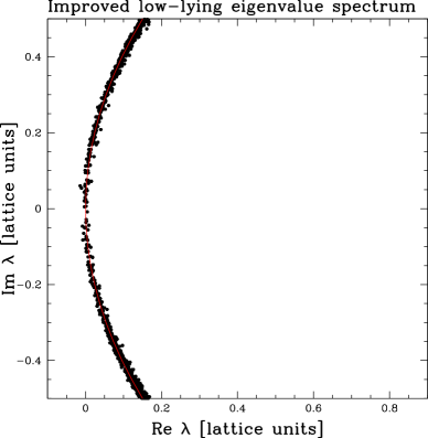
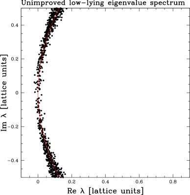
Figure 6: Physical branch of the spectrum of the Wilson-Dirac operator; 20 superimposed configurations (left) with and (right) without improvement ($14^{3}$ lattices with $g^{2}a=0.5$)

The disadvantage of Wilson fermions is that we must tune the fermion mass to remove an additive correction. To consistently improve the theory to eliminate all $O(a)$ errors we need to do this at the two loop level (see elliottmoore for a discussion). Here we present the calculation of the one-loop mass counterterm; in practice both one and two loop counterterms can be determined quite easily numerically by analyzing the low-lying eigenvalues in the Dirac operator spectrum at a few different lattice spacings.

The SW term modifies only the $\bar{\psi}A\psi$ vertex. Following closely the 4D treatment of Capitani:2002mp we determine the new three point vertex to be (with $\bar{\psi}(p)$, $\psi(p^{\prime})$ and $A(k{=}p^{\prime}{-}p)$)

$$\Big{(}V_{\mu}\Big{)}^{a}_{bc}(p,p^{\prime})=-gT^{a}_{bc}\Bigg{(}i\sigma_{\mu}\cos\frac{(p{+}p^{\prime})_{\mu}}{2}+\frac{r}{2}\widetilde{(p{+}p^{\prime})}_{\mu}+\frac{c_{sw}r}{4}[\hbox to0.0pt{\hbox to5.55557pt{\hfil/\hfil}\hss}\hat{k},\sigma_{\mu}]\cos\frac{k_{\mu}}{2}\Bigg{)}\,.$$ (9)

The one-loop bare mass counterterm required to tune the theory to its SUSY limit, for Wilson coefficient $r=1$, is

$$\delta m=\frac{g^{2}C_{A}}{4\pi}(-2.3260)=\frac{C^{2}_{A}}{2\pi\beta}(-2.3260)\,,$$ (10)

with $C_{A}$ the first Casimir of the adjoint representation of the gauge group - $C_{A}{=}N_{\rm c}$ for SU($N_{\rm c}$).

To eliminate all $O(a)$ errors it is also necessary to compute a 1-loop fermionic wave-function renormalization (which can be interpreted as an $O(a)$ multiplicative renormalization of the mass) and a 1-loop renormalization of the field strength (or equivalently of $g^{2}$, or equivalently of the lattice spacing). The contribution of bosonic loops to the gauge coupling renormalization was computed in Oa2 , and the fermionic contribution is not difficult. In the same notation as that previous work,

$${\cal L}_{\rm latt}(x)=\frac{2}{Z_{g}g^{2}a^{4}}\sum_{i<j}\,{\rm Tr}\>(1-P_{ij}(x))+Z_{\psi}\bar{\psi}\left(D_{W}+D_{sw}+\frac{Z_{m}}{Z_{\psi}}m+\frac{\delta m}{Z_{\psi}}\right)\psi\,,$$ (11)

where it was determined that

$$Z^{\rm bosonic}_{g}=1-\frac{ag^{2}}{4\pi}\left(\frac{2\pi}{9N_{\rm c}}(2N_{\rm c}^{2}-3)+N_{\rm c}\left(\frac{37\xi}{12}-\frac{\pi}{9}\right)\right)\quad\mbox{with}\quad\xi=0.152859325\,,$$ (12)

we have

$$\frac{Z_{m}}{Z_{\psi}} = 1-\frac{ag^{2}N_{\rm c}}{4\pi}e_{m}\qquad\mbox{with}\quad e_{m}=2.75066732(8)$$ (13)

$$\mbox{and}\qquad Z^{\rm total}_{g} = Z^{\rm bosonic}_{g}-\frac{ag^{2}N_{\rm c}}{4\pi}e_{g}\qquad\mbox{with}\quad e_{g}=0.204254488(7)\,.$$ (14)

To treat $N_{\rm f}$ fundamental representation fermions rather than one adjoint with a Majorana condition, replace $N_{\rm c}\rightarrow C_{\rm f}$ in the expression for $Z_{m}/Z_{\phi}$ and change $N_{\rm c}\rightarrow N_{\rm f}$ in the expression for $Z_{g}$ (the $1/2$ trace normalization group theory factor cancels a factor of 2 from not imposing the Majorana condition).

As already mentioned, $\delta m$ is easily measured nonperturbatively by - for example - looking at the lowest lying eigenvalues of the Dirac operator for a range of $\beta$ values and fitting to find what value of $\delta m$ is needed to get the zero imaginary part eigenvalues to have vanishing real part as well. To tune out the O($a$) error analytically would require a 2-loop determination of the fermion self energy, which is much more difficult.

The numerical implementation of the magnitude of the determinant is achieved by including $(\det{\cal D}^{\dagger}{\cal D})^{1/4}$ in the path integral, which can be accomplished by conventional pseudofermion techniques. There should be no issues with locality (we believe) because the operator’s spectrum is doubled, so the fourth root is actually well defined (up to a phase).

III.2 Evaluation of Chern-Simons number

Here we detail how to determine the Chern-Simons number of a 3-dimensional lattice configuration. Our approach is borrowed from an investigation of the electroweak sphaleron rate by one of us broken_sphaleron , but we summarize it here for completeness.

The literal definition of Chern-Simons number $N_{\rm CS}$ in terms of the integral of $F\wedge A-\frac{1}{3}A\wedge A\wedge A$, given in Eq. (II), is too gauge dependent and lattice spacing sensitive to be of much use, so we use instead the following (gauge invariant) properties of Chern-Simons number, which can be taken as a definition of $N_{\rm CS}$, modulo an integer:

• $N_{\rm CS}$ for the vacuum is 0 (modulo an integer); and

• the $N_{\rm CS}$ difference between two configurations is (modulo an integer) equal to the integral of $\epsilon^{\mu\nu\alpha\beta}\,{\rm Tr}\>F_{\mu\nu}F_{\alpha\beta}/32\pi^{2}$ along a path through configuration space connecting those configurations.

The second point requires some clarification. As previously discussed, given two 3D configurations $A^{i}_{1}({\bf x})$, $A^{i}_{2}({\bf x})$, one can find a path connecting them through gauge field configuration space; that is, one can find $A^{i}({\bf x},\tau)$ with $\tau\in[0,1]$ an affine parameter and $A^{i}({\bf x},0)=A^{i}_{1}({\bf x})$, $A^{i}({\bf x},1)=A^{i}_{2}({\bf x})$. We may think of the path as a 4-dimensional gauge field configuration, with $\tau$ as the fourth coordinate, $D_{0}\equiv D_{\tau}$, and $F_{0i}=i[D_{0},D_{i}]$. The $N_{\rm CS}$ difference between two configurations is the integral

$$N_{\rm CS}(A_{2})-N_{\rm CS}(A_{1})=\int d^{3}x\int_{0}^{1}d\tau\epsilon_{ijk}\frac{\,{\rm Tr}\>F_{0i}F_{jk}}{8\pi^{2}}\,.$$ (15)

We have not specified how $A_{0}$ is to be chosen along the $\tau$ direction, but this turns out not to matter; a different choice leads to a change in $F_{0i}$ of $D_{i}\delta A_{0}$, but the $D_{i}$ can be integrated by parts onto $F_{jk}$ and $\epsilon_{ijk}D_{i}F_{jk}$ vanishes by the Bianchi identity. The idea is then to define $N_{\rm CS}$ for a configuration (modulo an integer) by finding a path from that configuration to the vacuum and integrating $F\tilde{F}$ along that path.

The complication in using this approach to define $N_{\rm CS}$ on the lattice is that there is no lattice definition of the field strength $F_{\mu\nu}$ which satisfies the Bianchi identity; therefore the procedure is ambiguous. Further, no specific prescription for choosing $A_{0}$ generically leads to an integer $N_{\rm CS}$ around a closed loop. There are mathematically rigorous Luscher82 ; Woit85 ; Stone84 and numerically implementable Hetrick ; DeGrand methods to find the integer value around closed loops, but these are not helpful here, since we really want the value on a path with distinct beginning and end points. The trick instead is to note that the problems with lattice implementations of $F\tilde{F}$ arise when the fields are “coarse” (plaquettes far from identity, most of excitations at the lattice spacing scale). We can define $N_{\rm CS}$ uniquely by choosing any unique prescription for a path from a configuration to the vacuum. We can ensure that the result is as close as possible to the continuum meaning of $N_{\rm CS}$ if our unique prescription is one which quickly smooths out the lattice-spacing scale fluctuations in the gauge field configuration. The early “smoothing out” part of the path then contributes a small UV “lattice artifact” contribution to $N_{\rm CS}$ and the remaining path gives a contribution which closely resembles the continuum value of $N_{\rm CS}$ for this configuration.

A good choice is the “cooling path” or gradient decent under the energy,

$$D_{\tau}A^{i}(x,\tau)=-\frac{\partial H[A({\bf x},\tau)]}{\partial A^{i}(x,\tau)}\,,\qquad H[A]\equiv\int d^{3}y\;\frac{1}{2}\,{\rm Tr}\>F^{2}_{ij}[A({\bf y},\tau)]\,.$$ (16)

We use a Symanzik Symanzik or “rectangle-improved” definition of $H$ and of the field strength appearing in $F\tilde{F}$, as described in broken_sphaleron , which also shows extensive tests of the approach.

To summarize, the procedure is to determine the Chern-Simons number of a lattice configuration by integrating $F\tilde{F}$ along the “cooling” or gradient-decent path through configurations to the vacuum. The procedure is unique and gives an answer which is continuous over the space of gauge field configurations except at a “sphaleron” separatrix, where it is discontinuous by (almost exactly) an integer. If Markov-chain configurations are tightly enough sampled, one can determine the integer part by continuity.

On fine lattices this definition of Chern-Simons number should correctly reproduce the continuum notion up to corrections suppressed by two powers of the lattice spacing.

A straightforward alternative method to implement integer Chern-Simons numbers would be to evaluate the phase in the determinant of a fundamental representation Wilson fermion with a negative mass of order the lattice spacing (so the origin of the complex plane is inside the leftmost “circle” in Fig. 4). This method would be numerically much less efficient, since the numerical effort in taking a determinant rises as the third power of the number of lattice points or $a^{9}$, while the approach presented only grows worse as $a^{5}$ and can be reduced to $a^{3}$ through the careful use of blocking broken_sphaleron .

III.3 Fermionic phase

Since in practice only the magnitude of the rooted fermion determinant can be included dynamically in a lattice simulation, we must still describe a prescription for assigning to the Wilson-Dirac operator a phase for each field configuration in order to complete the prescription for the discretization of the theory.

One approach to do this would be to explicitly evaluate the (complex) determinant of ${\cal D}$ for each configuration in the Markov chain and then halve the phase, fixing the sign ambiguity by using a tightly sampled Markov chain and demanding continuity. Then one must subtract the Chern-Simons phase contribution from the “return loop” discussed in Subsection II.2. This approach is correct but numerically expensive.

After correcting for the Chern-Simons term induced by the “return loop” this phase is dominated by the contributions of the low lying eigenvalues, so we can develop a more efficient procedure by focusing on determining the phase arising from these eigenvalues. Since this point is key to our approach we should explain it in a little detail. Look again at Fig. 6. In the continuum limit the eigenvalues will lie, not on an arc, but on a straight line with real part $m$ and imaginary part set by the eigenvalue under the $\hbox to0.0pt{\hbox to8.55695pt{\hfil/\hfil}\hss}D$ operator (for the free theory, by $k$). At large eigenvalue the weak-coupling approximation is valid (since the theory is super-renormalizable this is true by a power of the eigenvalue). The density of eigenvalues therefore scales with the free theory density of states, $k^{2}dk$. An eigenvalue’s phase difference from $\pm\frac{\pi}{2}$ is $\tan^{-1}(m/k)$, so naively the phase arising from large eigenvalues could be large. What is important, though, is the phase difference configuration by configuration, and this becomes small, essentially because the large eigenvalues do not change very much as a function of the gauge field. To see this, note that the large eigenvalues represent short-range physics. The influence on the effective IR behavior can be expanded as Wilsonian renormalization of effective IR operators. The lowest order parity-odd operator is the Chern-Simons term; all others are higher by at least two powers of derivatives and therefore suppressed by at least $g^{4}/k^{2}$. Since we are allowing $O(a^{2})$ errors, the only operator we need to incorporate correctly from the large $k$ eigenvalues is therefore their contribution to the Chern-Simons term. Therefore our strategy will be to include low eigenvalues’ phases explicitly and to determine the phase contribution of large eigenvalues in terms of their contribution to an effective Chern-Simons term.

We can extract the smallest $M$ eigenvalues using the Arnoldi method at much less numerical effort than is required to determine the full determinant. Each such eigenvalue $\lambda_{i}$ of the Wilson-Dirac operator with renormalized mass $m$ takes a value in the complex plane, $(r_{i},i_{i})$. In the continuum limit the real parts $r_{i}$ always equal $m$. At finite lattice spacing there will be $O(g^{4}a^{2})$ and $O(i^{2}a^{2})$ deviations in the real part. (There would be $O(g^{2}a)$ deviations arising from the dimension 5 operator $\bar{\psi}\sigma_{\mu\nu}F^{\mu\nu}\psi$ had we not included the SW term.) We “clean” the low lying eigenvalues by projecting them to the $r=m$ axis, see Fig. 7. Each eigenvalue then contributes a phase

$$\phi_{i}=\tan^{-1}\left(\frac{\sqrt{(r_{i}-m)^{2}+i^{2}_{i}}}{m}\right)\,.$$ (17)

This amounts to projecting the physical branch of the Wilson-Dirac spectrum onto the axis of the continuum spectrum and then calculating the phase as sketched in Fig. 7.

$\begin{array}[]{c@{\hspace{.6in}}c}\epsfbox{phase_projection.eps}\hfil\hskip 43.36243pt&\epsfbox{project_detail.eps}\end{array}$

Figure 7: Sketch of the projection for the phase prescription.

The idea is to incorporate the phase of all eigenvalues for which the angle $\phi_{i}$ lies in a range $[-\phi_{\rm max},\phi_{\rm max}]$. In the $a\rightarrow 0$ limit we must take $\phi_{\rm max}\rightarrow\frac{\pi}{2}$. This requires more eigenvalues at finer lattice spacing; this can be made more efficient by using the shifted Arnoldi method.

The Markov evolution of the gauge fields $U_{\mu}$ will move around the eigenvalues so that eigenvalues regularly move in and out of the “window” in which we explicitly include them. When an eigenvalue goes above or below $\phi_{\rm max}$, the phase we determine will abruptly change by $\mp\phi_{\rm max}$. Therefore each configuration along the Markov chain must be reasonably close to the last, so that these phases can be determined by continuity. The change in phase between neighboring configurations $U_{1,2}$ contributed by all eigenvalues lying above $\phi_{\rm max}$ and below $-\phi_{\rm max}$ is simply an effective Chern-Simons term, as discussed above. The size of the contribution can be determined by considering the amount of spectral flow due to a changing Chern-Simons number, and is well approximated by $2(\frac{\pi}{2}-\phi_{\rm max})N_{\rm c}\,(N_{\rm CS}(U_{2})-N_{\rm CS}(U_{1}))$. We have confirmed this in quenched simulations, for instance by analyzing the $\phi_{\rm max}$ dependence of the procedure and seeing that this contribution ensures independence on this artificial parameter. If we choose the vacuum with, for example, $N_{\rm CS}=0$ to have zero phase, then this prescription uniquely determines a phase for all configurations.

III.4 The sign (or phase) problem

Now that the appropriate implementations of the fermionic field content and the Chern-Simons term have been detailed there remains no fundamental barrier to the simulation of the theory and so we turn our attention to an important technical issue of the simulation.

The lattice simulation consists of replacing the path integral by a sum over a finite set of link field configurations that are distributed with a probability given by the Boltzmann factor for the theory, $|\exp(-S[U])|$. For complex action, the ensemble average for an observable ${\cal O}$ will be

$$\langle{\cal O}\rangle\approx\frac{\sum_{i=1}^{N}{\cal O}(U_{i})e^{i\phi_{i}}}{\sum_{i=1}^{N}e^{i\phi_{i}}}\,,$$ (18)

where $\phi=\arg\exp(-S[U])$. Obviously this leads to cancellations between link configurations from the sampling, and thus to a reduction in statistics. That is, for a sample of $N$ independent configurations, the error in the numerator scales as $\sqrt{N}$; but the denominator will be smaller than $N$, so the error in the operator will not be $1/\sqrt{N}$. This problem could be eliminated by performing “phase quenching” on the theory, but this does uncontrolled damage to the theory which in our case we believe is severe. Therefore we must face this phase cancellation issue.

To determine how bad the phase cancellations will be, we start by looking at the theory with very large fermion mass, so that the effect of integrating out the fermion is well approximated by a shift to the Chern-Simons coefficient, $k\to k-N_{\rm c}/2$. In large volumes, we expect that $N_{cs}$ will be Gaussian distributed around zero. The degree of phase cancellation is determined by how badly our determination of $1$ in the denominator of Eq. (18) is “suppressed”: all measurables must be scaled by the result of the partition function which we evaluate as $\langle 1\rangle$ with the average replaced by a sum on configurations with phases. Fluctuations go as $1/\sqrt{N}$ with $N$ the number of configurations (unless each configuration contributes better statistics–this depends on the measurable). The point is that these fluctuations are to be compared with an average value which suffers phase cancellation. We estimate this by doing the (Gaussian) integral over $N_{cs}$ to find how big the partition function actually is:

$$\langle 1\rangle=\int\frac{dN_{cs}}{\sqrt{2\pi\chi}}\exp(-i2\pi kN_{cs})\exp(-N_{cs}^{2}/2\chi)$$ (19)

with $\chi$ the variance of $N_{cs}$ and $k$ the effective Chern-Simons coefficient. The integral gives

$$\exp(-2\pi^{2}k^{2}\chi)\,.$$ (20)

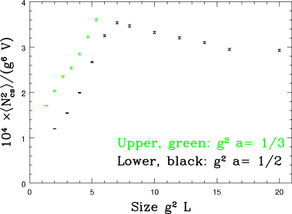
Figure 8: (color online) Variance of $N_{\rm CS}$ as a function of volume, for two lattice spacings, in quenched SU(2) gauge theory and using the definition of $N_{\rm CS}$ presented in the text.

Fig. 8 shows the dependence of $\chi/V$ on the volume of the lattice, in quenched simulations. As the figure shows, going to a finer lattice induces a constant shift in $\chi$, and the volume dependence becomes weak for boxes larger than about $8/g^{2}$. At this value, on a “reasonably fine” lattice of $g^{2}a=0.5$ [$\beta=8$], the $N_{\rm CS}$ variance is about .175, leading to a sign problem induced loss of statistical power of order $\exp(-2\pi^{2}k^{2}\times.175)=1/30$ for $k=1$. This volume is therefore at the limit of practicality. Statistical power falls exponentially if we try to make the volume any larger. However, a box of length $8/g^{2}$ is very large. The theory has a mass gap and the large volume limit should be approached rapidly in a box a few times longer than the longest correlation length. For the SU(2) theory, the lightest glueball mass is $m_{0^{++}}\simeq 1.66g^{2}$ Teper and the inverse correlation length involved in the Debye mass is $\simeq 1.14g^{2}$ Philipsen . These both suggest that the dominant physics is on quite short scales $\sim 1/g^{2}$, though the string tension suggests a longer correlation length $1/\sqrt{\sigma}\simeq 3/g^{2}$ Teper . Therefore this volume is probably sufficient to effectively achieve the continuum limit.

The sign problem grows more severe at large $k$, as indicated by Eq. (20). Fortunately the mass scales with $k$, so we can reduce the volume as $V\propto 1/k^{3}$ in the large $k$ limit. We must also tighten the lattice spacing $a$ to keep $ka$ fixed, and since $\langle N_{\rm CS}^{2}\rangle$ turns out to have a linear UV divergence (which causes the lattice spacing dependence observed in Fig. 8), this means that $\chi$ will scale as $V/a\sim k^{-2}$. In the large $k$ limit the severity of the sign problem therefore approaches a finite limit.

Fig. 8 is based on quenched configurations. When we include the effects of dynamical fermions, we expect the situation at small $k$ to improve for two reasons. The first is that inclusion of the magnitude of the determinant in the Boltzmann factor suppresses configurations with large $N_{\rm CS}$ (an effect we have observed in preliminary quenched simulations). This is not surprising since we know that Dirac operators for configurations with half-integer $N_{\rm CS}$ (sphalerons) have zero eigenvalues. We thus expect this suppression to be more effective at smaller fermion masses. We will not attempt to quantify this statement further.

The second reason is that the phase contributed by the determinant partially cancels against the phase from the Chern-Simons term. For large fermion mass, for example, we know from continuum methods that integrating out the fermion gives a shift in $k$ or, equivalently, a contribution to the partition function $\exp(i\pi N_{\rm c}N_{\rm CS})$. Furthermore, we have confirmed for the case of $N_{\rm c}{=}2$ Wilson-Dirac fermions – with the prescription described above for assigning determinant phases – that this is approximately the phase of the rooted fermion determinant for the relatively small masses ($k{=}1,2,3$) of interest here. An example is shown in Fig. 9 for $k{=}1$. In this case the cancellation of the phase in the partition function is nearly exact, and the phase problem disappears. Finally we remark that, in the algorithm for determining $N_{\rm CS}$, one can begin the integration of $F\tilde{F}$ after a short amount of cooling, eliminating the contribution from the most UV modes. This eliminates a lattice artifact “noise” contribution to $\chi$ but leaves that from interesting IR physics intact.

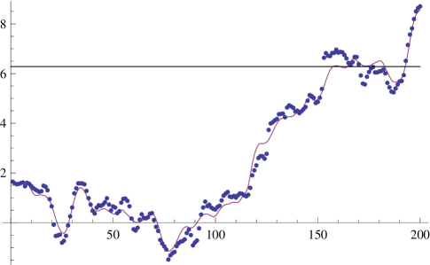
Figure 9: Evolution of the phase of the rooted fermion determinant over a Markov chain of length 200. The continuous line is $2\pi N_{cs}$. The system transitions through a sphaleron and subsequently fluctuates around the topologically distinct vacuum at $2\pi$.

IV Conclusion

Three dimensional minimally supersymmetric gauge theory can be implemented on the lattice. As we showed, this theory necessarily involves complex phases; the theory with vanishing Chern-Simons term and massless fermions is anomalous because the path integral is odd under parity transformations and the partition function therefore vanishes identically.

Our implementation has concentrated on numerical efficiency. Lattice spacing corrections should first occur at $O(a^{2})$. Fermions need only be implemented using the clover-improved Wilson method, not the much more expensive overlap method. The Chern-Simons phase can be determined without reference to fermionic operators, and the phase in the rooted Dirac determinant is determined by finding only the low lying eigenvalues using the Arnoldi method, rather than by taking the full determinant. This efficiency is important because the theory suffers from a sign problem which will make it difficult to take the large volume limit. We are guardedly optimistic that the sign problem will not be as severe as might be feared. First, the phase of the fermionic determinant and of the Chern-Simons term are of opposite sign and partially cancel. Second, when the Chern-Simons term is large, the theory is massive and the volume requirement should be reduced.

Now that an implementable method has been presented, it would be very interesting to study 3D ${\cal N}{=}1$ SYM on the lattice. In particular it would greatly improve our insight into nonperturbative supersymmetry breaking if we could study and (presumably) verify Witten’s conjectures regarding spontaneous SUSY breaking in this theory Witten3d .

Acknowledgements

We would like to thank Joel Giedt for useful conversations. JE thanks the University of Chicago physics department for their hospitality while this work was being prepared. This work was partially supported by grants from the National Science and Engineering Research Council of Canada (NSERC) and by le Fonds Québécois de la Recherche sur la Nature et les Technologies (FQRNT).

References

- (1) A. G. Cohen, D. B. Kaplan, E. Katz and M. Unsal, JHEP 0308, 024 (2003) [arXiv:hep-lat/0302017]; JHEP 0312, 031 (2003) [arXiv:hep-lat/0307012]; D. B. Kaplan and M. Unsal, JHEP 0509, 042 (2005) [arXiv:hep-lat/0503039].
- (2) S. Catterall, JHEP 0411, 006 (2004) [arXiv:hep-lat/0410052].
- (3) D. B. Kaplan, Phys. Lett. B 288, 342 (1992) [hep-lat/9206013].
- (4) R. Narayanan and H. Neuberger, Nucl. Phys. B 412, 574 (1994) [hep-lat/9307006].
- (5) G. T. Fleming, J. B. Kogut and P. M. Vranas, Phys. Rev. D 64, 034510 (2001) [hep-lat/0008009]; I. Campos et al. [DESY-Münster Collaboration], Eur. Phys. J. C 11, 507 (1999) [hep-lat/9903014]; R. Kirchner, I. Montvay, J. Westphalen, S. Luckmann and K. Spanderen [DESY-Münster Collaboration], Phys. Lett. B 446, 209 (1999) [hep-lat/9810062]; R. Kirchner, S. Luckmann, I. Montvay, K. Spanderen and J. Westphalen [DESY-Münster Collaboration] Nucl. Phys. Proc. Suppl. 73, 828 (1999) [hep-lat/9808024]; A. Donini, M. Guagnelli, P. Hernandez and A. Vladikas, Nucl. Phys. B 523, 529 (1998) [hep-lat/9710065]; J. Nishimura, Phys. Lett. B 406, 215 (1997) [arXiv:hep-lat/9701013]; K. Itoh, M. Kato, H. Sawanaka, H. So and N. Ukita, JHEP 0302, 033 (2003) [arXiv:hep-lat/0210049].
- (6) E. Witten, arXiv:hep-th/9903005.
- (7) A. N. Redlich, Phys. Rev. D 29, 2366 (1984).
- (8) E. Witten, Phys. Lett. B 117, 324 (1982).
- (9) M. F. Atiyah, V. K. Patodi, and I. M. Singer, Proc. Camb. Philos. Soc. 77 (1975) 43, 78 (1980) 2848, 79 (1976) 1.
- (10) B. Sheikholeslami and R. Wohlert, Nucl. Phys. B 259, 572 (1985).
- (11) C. Gattringer and I. Hip, Nucl. Phys. B 541, 305 (1999) [arXiv:hep-lat/9806032].
- (12) J. W. Elliott and G. D. Moore, PoS LAT2005, 245 (2006) [JHEP 0511, 010 (2005)] [arXiv:hep-lat/0509032].
- (13) S. Capitani, Phys. Rept. 382, 113 (2003) [arXiv:hep-lat/0211036].
- (14) G. D. Moore, Nucl. Phys. B 523, 569 (1998) [arXiv:hep-lat/9709053].
- (15) G. D. Moore, Phys. Rev. D 59, 014503 (1999) [arXiv:hep-ph/9805264].
- (16) M. Lüscher, Commun. Math. Phys. 85, 39 (1982).
- (17) P. Woit, Phys. Rev. Lett. 51, 638 (1983); Nucl. Phys. B 262, 284 (1985).
- (18) A. Phillips and D. Stone, TOPOLOGICAL Commun. Math. Phys. 103, 599 (1986).
- (19) P. de Forcrand, M. Garcia Perez, J. E. Hetrick and I. O. Stamatescu, Nucl. Phys. Proc. Suppl. 63, 549 (1998) [arXiv:hep-lat/9710001]; arXiv:hep-lat/9802017.
- (20) T. A. DeGrand, A. Hasenfratz and T. G. Kovacs, Nucl. Phys. B 505, 417 (1997) [arXiv:hep-lat/9705009].
- (21) K. Symanzik, Nucl. Phys. B 226, 187 (1983). K. Symanzik, Nucl. Phys. B 226, 205 (1983).
- (22) M. J. Teper, Phys. Rev. D 59, 014512 (1999) [arXiv:hep-lat/9804008].
- (23) M. Laine and O. Philipsen, Phys. Lett. B 459, 259 (1999) [arXiv:hep-lat/9905004].