Wightman function and scalar Casimir densities for a wedge with two cylindrical boundaries

Abstract

Wightman function, the vacuum expectation values of the field square and the energy-momentum tensor are investigated for a massive scalar field with general curvature coupling parameter inside a wedge with two coaxial cylindrical boundaries. It is assumed that the field obeys Dirichlet boundary condition on bounding surfaces. The application of a variant of the generalized Abel-Plana formula enables to extract from the expectation values the contribution corresponding to the geometry of a wedge with a single shell and to present the interference part in terms of exponentially convergent integrals. The local properties of the vacuum are investigated in various asymptotic regions of the parameters. The vacuum forces acting on the boundaries are presented as the sum of self-action and interaction terms. It is shown that the interaction forces between the separate parts of the boundary are always attractive. The generalization to the case of a scalar field with Neumann boundary condition is discussed.

PACS numbers: 11.10.Kk, 03.70.+k

1 Introduction

The nontrivial properties of the vacuum state are among the most important predictions in quantum field theory. These properties are manifested in the response of the vacuum to external influences such as external fields. A simple model of the influence is realized by imposing prescribed boundary conditions on the field operator. The distortion of the spectrum for the zero-point fluctuations of a quantum field by these conditions results in the shifts in the vacuum expectation values of physical observables, such as the vacuum energy density and stresses, and induces vacuum forces acting on constraining boundaries. This is the well known Casimir effect (see [1, 2, 3, 4] and references therein). The Casimir effect is common to all systems characterized by fluctuating quantities and has important implications on all scales, from cosmological to subnuclear. In addition to its fundamental interest this effect also plays an important role in the fabrication and operation of nano- and micro-scale mechanical systems and has become an increasingly popular topic in quantum field theory.

An interesting topic in the investigations of the Casimir effect has always been the dependence of the physical characteristics of the vacuum on the geometry of constraining boundaries. Analytic results can usually be found only for highly symmetric geometries including planar, spherically and cylindrically symmetric boundaries. Recently exact results for the Casimir force in geometries of a sphere and a cylinder above a plate are obtained in [5, 6] (see also [7]). Aside from their own theoretical and experimental interest, the problems with this type of boundaries are useful for testing the validity of various approximations used to deal with more complicated geometries. In the present paper we consider a less symmetric exactly solvable geometry of boundaries which is a combination of a wedge with coaxial cylindrical shells. The Casimir effect for wedge-shaped regions is well investigated in literature [1, 8, 9, 10, 11, 12]. For a conformally coupled scalar and electromagnetic fields the vacuum expectation value of the energy-momentum tensor inside the wedge is azimuthal symmetric. In particular, the vacuum energy-momentum tensor is finite everywhere apart points on the edge. This property is a direct consequence of the conformal invariance in the corresponding problems and does not take place for a non-conformally coupled scalar field. For a scalar field with an arbitrary curvature coupling parameter satisfying Dirichlet boundary condition on the wedge sides the vacuum energy-momentum tensor is evaluated in [13, 14]. In addition to the azimuthal dependence this tensor, unlike to the case of conformally coupled fields, is also non-diagonal with nonzero azimuthal-radial off-diagonal component.

The investigations of quantum effects for cylindrical boundaries have received a great deal of attention. In addition to traditional problems of quantum electrodynamics under the presence of material boundaries, the Casimir effect for cylindrical geometries is also important in the flux tube models of confinement [15, 16] and for determining the structure of the vacuum state in interacting field theories [17]. The calculation of the vacuum energy for the electromagnetic field with boundary conditions defined on a cylinder turned out to be technically a more involved problem than the analogous one for a sphere. First the Casimir energy of an infinite perfectly conducting cylindrical shell has been calculated in Ref. [18] by introducing ultraviolet cutoff and later the corresponding result was derived by using other methods [19, 20, 21]. The local characteristics of the corresponding electromagnetic vacuum such as energy density and vacuum stresses are considered in [22] for the interior and exterior regions of a conducting cylindrical shell, and in [23] for the region between two coaxial shells (see also [24]). The electromagnetic vacuum forces acting on the boundaries in the geometry of two cylinders are also considered in Refs. [25]. In Ref. [26] scalar vacuum densities and the zero-point energy for general Robin boundary condition on a cylindrical surface in arbitrary number of spacetime dimensions are studied for massive scalar field with general curvature coupling parameter. The corresponding problem for the geometry of two coaxial cylindrical shells is considered in [27]. A large number of papers is devoted to the investigation of the various aspects of the Casimir effect for a dielectric cylinder (see, for instance, [4, 28] and references therein).

In the geometry of a wedge with coaxial cylindrical boundary the modes are still factorizable for both scalar and electromagnetic fields and the corresponding problems are exactly solvable. The total Casimir energy of a semi-circular infinite cylindrical shell with perfectly conducting walls is considered in [29] by using the zeta function technique. For a scalar field with an arbitrary curvature coupling parameter obeying Dirichlet boundary condition the Wightman function, the vacuum expectation values of the field square and the energy-momentum tensor in the geometry of a wedge with an arbitrary opening angle and with a cylindrical boundary are investigated in [13, 14]. The corresponding Casimir densities for the electromagnetic field with perfect conductor boundary conditions on bounding surfaces are considered in [30]. The closely related problem with a cylindrical shell in the geometry of a cosmic string is discussed in [31, 32] for scalar and electromagnetic fields. In both scalar and electromagnetic cases the application of a variant of the generalized Abel-Plana formula [24] enables to extract from the vacuum expectation values the parts corresponding to the geometry of a wedge without the cylindrical shell and to present the shell induced parts in terms of rapidly converging integrals. This geometry is also interesting from the point of view of general analysis for surface divergences in the expectation values of local physical observables for boundaries with discontinuities. The nonsmoothness of the boundary generates additional contributions to the heat kernel coefficients (see, for instance, the discussion in [28, 33, 34, 35] and references therein).

In this paper we investigate one-loop vacuum quantum effects for a scalar field in the geometry of a wedge with two coaxial cylindrical shells assuming Dirichlet boundary condition on bounding surfaces. This geometry generalizes various special cases previously considered in literature for wedge-shaped and cylindrical boundaries. In addition, we also study the role of nonzero mass of the field quanta. The presence of boundaries eliminates the translational invariance and as a result the properties of the vacuum are nonuniform. The most important quantities characterizing the local properties of the vacuum are the expectation values of the field square and the energy-momentum tensor. In addition to describing the physical structure of the quantum field at a given point, the energy-momentum tensor acts as the source of gravity in the Einstein equations. It therefore plays an important role in modelling a self-consistent dynamics involving the gravitational field. As the first step for the investigation of vacuum densities we evaluate the positive frequency Wightman function. This function gives comprehensive insight into vacuum fluctuations and determines the response of a particle detector of the Unruh-DeWitt type. Having the vacuum energy-momentum tensor we can derive the vacuum forces acting on constraining boundaries evaluating the vacuum stresses at points on the bounding surfaces. As we will see below, in the geometry under consideration these forces are position dependent on the boundary and cannot be obtained by the global method using the total Casimir energy (on the advantages of the local method see also [36]). In the limiting case from the results of the present paper the local vacuum densities are obtained for the geometry of a rectangular waveguide (for the local analysis of quantum fields confined in rectangular cavities see [36, 37, 38]).

The paper is organized as follows. The next section is devoted to the evaluation of the Wightman function for a massive scalar field in the region bounded by two cylindrical shells and by the wedge walls. This function is decomposed into three parts: the first one corresponds to the geometry of a wedge without cylindrical shells, the second one is induced by a single cylindrical shell when the second shell is absent, and the third one is induced by the presence of the second shell. By using the formula for the Wightman function, in section 3 the vacuum expectation values of the field square and the energy-momentum tensor are evaluated and their behavior is investigated in various asymptotic regions of the parameters. In section 4 we consider the vacuum forces acting on bounding surfaces. For separate boundary elements these forces are decomposed into self-action and interaction parts. The interaction forces are investigated in detail and numerical examples are presented. On the example of interaction forces we also demonstrate the limiting transition to the geometry of a rectangular waveguide. Finally, the results are summarized and discussed in section 5.

2 Wightman function

We consider a real scalar field $\varphi$ inside a wedge with opening angle $\phi_{0}$ and with two coaxial cylindrical shells of radii $a$ and $b$, $a<b$ (see figure 1). For the field with curvature coupling parameter $\xi$ the corresponding field equation has the form

$$\left(\nabla^{i}\nabla_{i}+\xi R+m^{2}\right)\varphi\left(x\right)=0,$$ (1)

where $R$ is the curvature scalar for a $(D+1)$-dimensional background spacetime, $\nabla_{i}$ is the covariant derivative operator. For special cases of minimally and conformally coupled scalars one has $\xi=0$ and $\xi=\xi_{D}\equiv(D-1)/4D$, respectively. Here we will assume that the background spacetime is flat and, hence, in Eq. (1) we have $R=0$. As a result the eigenmodes are independent of the curvature coupling parameter. However, the local characteristics of the vacuum such as the energy density and vacuum stresses depend on this parameter. In accordance with the problem symmetry we will use cylindrical coordinates $\left(r,\phi,z_{1},...,z_{N}\right)$,  $N=D-2$, and will assume that the field obeys Dirichlet boundary conditions on bounding surfaces:

$$\varphi|_{r=j}=\varphi|_{\phi=0}=\varphi|_{\phi=\phi_{0}}=0,\;j=a,b.$$ (2)

These boundary conditions modify the spectrum of the zero-point fluctuations compared with the case of free space and change the physical properties of the vacuum. Among the most important characteristics of the vacuum are the expectation values of the field square and the energy-momentum tensor. These expectation values can be obtained from two-point functions in the coincidence limit. As a two-point function here we will consider the positive frequency Wightman function $\left\langle 0|\varphi(x)\varphi(x^{\prime})|0\right\rangle$, where $|0\rangle$ is the amplitude for the vacuum state. This function also determines the response of Unruh-DeWitt type particle detectors [39]. Here we consider the spatial region $0\leqslant\phi\leqslant\phi_{0}$, $a\leqslant r\leqslant b$. The formulae for the regions $r\leqslant a$ and $r\geqslant b$ are obtained in limiting cases. Note that by using the corresponding formulae we can discuss various combinations of boundaries in the regions $0\leqslant\phi\leqslant\phi_{0}$ and $\phi_{0}\leqslant\phi\leqslant 2\pi$. For example, we can consider the situation with two cylindrical shells in the first region and without shells in the second one.

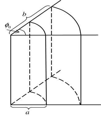
Figure 1: Geometry of a wedge with two coaxial cylindrical boundaries.

By expanding the field operator and using the standard commutation relations, the positive frequency Wightman function is presented as a sum over the eigenmodes:

$$\left\langle 0|\varphi(x)\varphi(x^{\prime})|0\right\rangle=\sum_{\alpha}\varphi_{\alpha}(x)\varphi_{\alpha}^{\ast}(x),$$ (3)

where $\left\{\varphi_{\alpha}(x),\varphi_{\alpha}^{\ast}(x)\right\}$  is a complete orthonormal set of positive and negative frequency solutions to the field equation satisfying boundary conditions (2). In the region between the cylindrical shells, $a\leqslant r\leqslant b$, the eigenfunctions are specified by the set of quantum numbers $\alpha=(n,\gamma,\mathbf{k})$,$~{}\ n=1,2,\cdots$, and have the form

$$\varphi_{\alpha}(x)=\beta_{\alpha}g_{qn}(\gamma a,\gamma r)\sin(qn\phi)\exp\left(i\mathbf{kr}_{\parallel}-i\omega t\right),$$ (4)

where

$$\omega=\sqrt{\gamma^{2}+k_{m}^{2}},\;k_{m}^{2}=|\mathbf{k}|^{2}+m^{2},\ q=\pi/\phi_{0},$$

and $\mathbf{r}_{\parallel}=\left(z_{1},...,z_{N}\right)$, $\mathbf{k}=(k_{1},\ldots,k_{N})$, $-\infty<k_{j}<\infty$. In formula (4) we have introduced the notation

$$g_{qn}(\gamma a,\gamma r)=Y_{qn}(\gamma a)J_{qn}(\gamma r)-J_{qn}(\gamma a)Y_{qn}(\gamma r),$$ (5)

with $J_{qn}(z)$ and $Y_{qn}(z)$ being the Bessel and Neumann functions. The eigenfunctions $\varphi_{\alpha}(x)$ defined by (4) satisfy the boundary conditions on the inner shell and on the wedge sides. The eigenvalues for the quantum number $\gamma$ are quantized by boundary condition (2) on the surface $r=b$ and are solutions of the equation

$$J_{qn}(\gamma a)Y_{qn}(\gamma b)-Y_{qn}(\gamma a)J_{qn}(\gamma b)=0.$$ (6)

In the discussion below the corresponding positive roots we will denote by $\gamma a=\sigma_{qn,l}$, $l=1,2,\ldots$, assuming that they are arranged in the ascending order, $\sigma_{qn,l}<\sigma_{qn,l+1}$.

The normalization coefficient $\beta_{\alpha}$ in (4) is found from the standard orthonormality condition for the eigenfunctions:

$$\int d^{N}\mathbf{r}_{\parallel}\int_{a}^{b}dr\,r\int_{0}^{\phi_{0}}d\phi\,\varphi_{\alpha}(x)\varphi_{\alpha^{\prime}}^{\ast}(x)=\frac{1}{2\omega}\delta_{nn^{\prime}}\delta_{ll^{\prime}}\delta(\mathbf{k-k}^{\prime}).$$ (7)

By making use of the standard integral for cylinder functions (see, for instance, [40]), one finds

$$\beta_{\alpha}^{2}=\frac{\pi^{2}q\gamma T_{qn}^{ab}(\gamma a)}{(2\pi)^{D-1}\omega a},$$ (8)

with the notation

$$T_{\nu}^{ab}(z)=\frac{z}{J_{\nu}^{2}(z)/J_{\nu}^{2}(\eta z)-1},\;\eta=b/a.$$ (9)

The substitution of eigenfunctions (4) into mode-sum formula (3) leads to the following expression for the positive frequency Wightman function

$$\left\langle 0|\varphi(x)\varphi(x^{\prime})|0\right\rangle = \frac{\pi^{2}q}{a}\int d^{N}\mathbf{k}\sum_{n=1}^{\infty}\sum_{l=1}^{\infty}\frac{zg_{qn}(z,zr/a)g_{qn}(z,zr^{\prime}/a)}{(2\pi)^{D-1}\sqrt{z+k_{m}^{2}a^{2}}}$$ (10)

$$\times\sin(qn\phi)\sin(qn\phi^{\prime})\exp(i\mathbf{k}\Delta\mathbf{r}_{\parallel}-i\omega\Delta t)T_{qn}^{ab}(z)\big{|}_{z=\sigma_{n,l}},$$

where $\Delta\mathbf{r}_{\parallel}=\mathbf{r}_{\parallel}-\mathbf{r}_{\parallel}^{\prime}$ and $\Delta t=t-t^{\prime}$. As the expressions for the eigenmodes $\sigma_{n,l}$ are not explicitly known, formula (10) for the Wightman function is not convenient. In addition, the separate terms in the sum are highly oscillatory for large values of quantum numbers. For the further evaluation of the summation over $l$ we apply formula [24]

$$\frac{\pi^{2}}{2}\sum_{l=1}^{\infty}h(\sigma_{qn,l})T_{qn}^{ab}(\sigma_{n,l}) = \int_{0}^{\infty}\frac{h(x)dx}{J_{qn}^{2}(x)+Y_{qn}^{2}(x)}$$ (11)

$$-\frac{\pi}{4}\int_{0}^{\infty}dx\,\Omega_{a,qn}(x,\eta x)\left[h(xe^{\pi i/2})+h(xe^{-\pi i/2})\right],$$

which is a direct consequence of the generalized Abel-Plana formula (for applications of the generalized Abel-Plana formula in investigations of the vacuum densities in the Casimir effect see also [41]). In (11)

$$\Omega_{a,qn}(x,y)=\frac{K_{qn}(y)/K_{qn}(x)}{K_{qn}(x)I_{qn}(y)-K_{qn}(y)I_{qn}(x)},$$ (12)

and $I_{qn}(x)$, $K_{qn}(x)$ are the modified Bessel functions.

As a function $h(x)$ in summation formula (11) we choose

$$h(x)=\frac{xg_{qn}(x,xr/a)g_{qn}(x,xr^{\prime}/a)}{\sqrt{x^{2}+k_{m}^{2}a^{2}}}\exp(-i\Delta t\sqrt{x^{2}/a^{2}+k_{m}^{2}}).$$ (13)

The corresponding conditions for this formula to be valid are satisfied if $r+r^{\prime}+|\Delta t|<2b$. In particular, this is the case in the coincidence limit $t=t^{\prime}$ for the region under consideration. As a result, the Wightman function is presented in the form

$$\left\langle 0|\varphi(x)\varphi(x^{\prime})|0\right\rangle = \frac{q}{2^{D-2}\pi^{D-1}}\sum_{n=1}^{\infty}\sin(qn\phi)\sin(qn\phi^{\prime})\int d^{N}\mathbf{k}\,e^{i\mathbf{k}\Delta\mathbf{r}_{\parallel}}$$ (14)

$$\times\Bigg{\{}\int_{0}^{\infty}dx\frac{h(x)/a}{J_{qn}^{2}(x)+Y_{qn}^{2}(x)}-\frac{2}{\pi}\int_{k_{m}}^{\infty}dx\frac{x\Omega_{a,qn}(ax,bx)}{\sqrt{x^{2}-k_{m}^{2}}}$$

$$\times G_{qn}(ax,rx)G_{qn}(ax,r^{\prime}x)\cosh(\Delta t\sqrt{x^{2}-k_{m}^{2}})\Bigg{\}},$$

where $h(x)$ is defined by (13) and we have introduced the notation

$$G_{qn}(x,y)=K_{qn}(x)I_{qn}(y)-I_{qn}(x)K_{qn}(y).$$ (15)

In the limit $b\rightarrow\infty$ the second term in figure braces on the right of (14) vanishes, whereas the first term does not depend on $b$. It follows from here that the part with the first term presents the Wightman function for the geometry of a wedge with a single cylindrical shell of radius $a$. The corresponding problem for a massless scalar field is investigated in [14]. For points $r<b$ the second term in figure braces on the right of (14) is finite in the coincidence limit and, hence, the renormalization procedure for the VEVs of the field square and the energy-momentum tensor is reduced to the corresponding procedure for the geometry with a single shell. In addition, in the coincidence limit of the arguments the $x$-integral in (14) is exponentially convergent in the upper limit.

In formula (14), the part corresponding to the geometry with a single cylindrical shell with radius $a$ can be further transformed by using the identity

$$\frac{g_{qn}(x,xr/a)g_{qn}(x,xr^{\prime}/a)}{J_{qn}^{2}(x)+Y_{qn}^{2}(x)} = J_{qn}(xr/a)J_{qn}(xr^{\prime}/a)-\frac{1}{2}\sum\limits_{\sigma=1}^{2}\frac{J_{qn}(x)}{H_{qn}^{(\sigma)}(x)}$$ (16)

$$\times H_{qn}^{(\sigma)}(xr/a)H_{qn}^{(\sigma)}(xr^{\prime}/a),$$

where $H_{qn}^{(\sigma)}(x)$, $\sigma=1,2$, are the Hankel functions. In the corresponding integral over $x$ with the second term on the right of (16) we rotate the integration contour by the angle $\pi/2$ for $\sigma=1$ and by the angle $-\pi/2$ for $\sigma=2$. Due to the well known properties of the Hankel functions, under the condition $r+r^{\prime}-|\Delta t|>2a$, the integrals over the arcs of the circle with large radius vanish, whereas the integrals over $(0,iak_{m})$ and $(0,-iak_{m})$ cancel out. Introducing the Bessel modified functions one obtains

$$\int_{0}^{\infty}dz\frac{h(x)/a}{J_{qn}^{2}(x)+Y_{qn}^{2}(x)} = \int_{0}^{\infty}dx\,x\frac{J_{qn}(xr)J_{qn}(xr^{\prime})}{\sqrt{x^{2}+k_{m}^{2}}}\exp(-i\Delta t\sqrt{x^{2}+k_{m}^{2}})$$ (17)

$$-\frac{2}{\pi}\int_{k_{m}}^{\infty}dx\frac{xI_{qn}(ax)}{K_{qn}(ax)}\frac{K_{qn}(xr)K_{qn}(xr^{\prime})}{\sqrt{x^{2}-k_{m}^{2}}}\cosh(\Delta t\sqrt{x^{2}-k_{m}^{2}}).$$

By taking into account this relation, the Wightman function is presented in the form

$$\left\langle 0|\varphi(x)\varphi(x^{\prime})|0\right\rangle = \left\langle\varphi(x)\varphi(x^{\prime})\right\rangle_{0}+\left\langle\varphi(x)\varphi(x^{\prime})\right\rangle_{a}-\frac{q}{2^{D-3}\pi^{D}}\sum_{n=1}^{\infty}\sin(qn\phi)\sin(qn\phi^{\prime})\,$$ (18)

$$\times\int d^{N}\mathbf{k}e^{i\mathbf{k}\Delta\mathbf{r}_{\parallel}}\int_{k_{m}}^{\infty}dx\,x\frac{\Omega_{a,qn}(ax,bx)}{\sqrt{x^{2}-k_{m}^{2}}}G_{qn}(ax,rx)G_{qn}(ax,r^{\prime}x)$$

$$\times\cosh(\Delta t\sqrt{x^{2}-k_{m}^{2}}).$$

In this formula,

$$\left\langle\varphi(x)\varphi(x^{\prime})\right\rangle_{0} = \frac{q}{2^{D-2}\pi^{D-1}}\sum_{n=1}^{\infty}\sin(qn\phi)\sin(qn\phi^{\prime})\int d^{N}\mathbf{k}\,e^{i\mathbf{k}\Delta\mathbf{r}_{\parallel}}$$ (19)

$$\times\int_{0}^{\infty}dx\,x\frac{J_{qn}(xr)J_{qn}(xr^{\prime})}{\sqrt{x^{2}+k_{m}^{2}}}\exp(-i\Delta t\sqrt{x^{2}+k_{m}^{2}}),$$

is the Wightman function for the wedge without cylindrical boundaries, and

$$\left\langle\varphi(x)\varphi(x^{\prime})\right\rangle_{a} = -\frac{q}{2^{D-3}\pi^{D}}\sum_{n=1}^{\infty}\sin(qn\phi)\sin(qn\phi^{\prime})\int d^{N}\mathbf{k}\,e^{i\mathbf{k}\Delta\mathbf{r}_{\parallel}}$$ (20)

$$\times\int_{k_{m}}^{\infty}dx\,x\frac{I_{qn}(ax)}{K_{qn}(ax)}\frac{K_{qn}(xr)K_{qn}(xr^{\prime})}{\sqrt{x^{2}-k_{m}^{2}}}\cosh(\Delta t\sqrt{x^{2}-k_{m}^{2}}),$$

is the part of the Wightman function induced by a single cylindrical shell with radius $a$ in the region $r>a$. Hence, the last term on the right of (18) is induced by the presence of the second shell with radius $b$.

An equivalent form for the Wightman function is obtained from (18) by using the identity

$$\sum_{j=a,b}n_{j}\Omega_{j,qn}(ax,bx)G_{qn}(jx,xr)G_{qn}(jx,xr^{\prime})$$ (21)

$$= \frac{K_{qn}(bx)}{I_{qn}(bx)}I_{qn}(xr)I_{qn}(xr^{\prime})-\frac{I_{qn}(ax)}{K_{qn}(ax)}K_{qn}(xr)K_{qn}(xr^{\prime}),$$

with the notations $n_{a}=1$, $n_{b}=-1$, and

$$\Omega_{b,qn}(x,y)=\frac{I_{qn}(x)/I_{qn}(y)}{K_{qn}(x)I_{qn}(y)-K_{qn}(y)I_{qn}(x)}.$$ (22)

This leads to the following representation for the Wightman function

$$\left\langle 0|\varphi(x)\varphi(x^{\prime})|0\right\rangle = \left\langle\varphi(x)\varphi(x^{\prime})\right\rangle_{0}+\left\langle\varphi(x)\varphi(x^{\prime})\right\rangle_{b}-\frac{q}{2^{D-3}\pi^{D}}\sum_{n=1}^{\infty}\sin(qn\phi)\sin(qn\phi^{\prime})\,$$ (23)

$$\times\int d^{N}\mathbf{k}e^{i\mathbf{k}\Delta\mathbf{r}_{\parallel}}\int_{k_{m}}^{\infty}dx\,x\frac{\Omega_{b,qn}(ax,bx)}{\sqrt{x^{2}-k_{m}^{2}}}G_{qn}(bx,xr)G_{qn}(bx,xr^{\prime})$$

$$\times\cosh(\Delta t\sqrt{x^{2}-k_{m}^{2}}).$$

In this formula,

$$\left\langle\varphi(x)\varphi(x^{\prime})\right\rangle_{b} = -\frac{q}{2^{D-3}\pi^{D}}\sum_{n=1}^{\infty}\sin(qn\phi)\sin(qn\phi^{\prime})\int d^{N}\mathbf{k}\,e^{i\mathbf{k}\Delta\mathbf{r}_{\parallel}}$$ (24)

$$\times\int_{k_{m}}^{\infty}dx\,x\frac{K_{qn}(bx)}{I_{qn}(bx)}\frac{I_{qn}(xr)I_{qn}(xr^{\prime})}{\sqrt{x^{2}-k_{m}^{2}}}\cosh(\Delta t\sqrt{x^{2}-k_{m}^{2}})$$

is the part induced by a single cylindrical shell of radius $b$ in the region $r<b$ and the last term on the right is induced by the presence of the second shell. Note that formulae (20) and (24) are related by the interchange $a\rightleftarrows b$, $I_{n}\rightleftarrows K_{n}$. For a massless scalar field these formulae are derived in [14].

3 VEVs of the field square and the energy-momentum tensor

3.1 Field square

In this section we consider the VEVs for the field square and the energy-momentum tensor in the region between the cylindrical shells. The VEV of the field square is obtained from the Wightman function in the coincidence limit of the arguments. In this limit and for points away from the boundaries the divergences are contained in the term $\left\langle\varphi(x)\varphi(x^{\prime})\right\rangle_{0}$ only. The corresponding renormalization procedure is realized by subtracting the part for the Minkowskian spacetime without boundaries. By using decompositions (18) and (23) for the Wightman function and taking the coincidence limit of the arguments, for the renormalized VEV of the field square one finds

$$\langle\varphi^{2}\rangle_{\mathrm{ren}}=\langle\varphi^{2}\rangle_{0,\mathrm{ren}}+\langle\varphi^{2}\rangle_{j}+\langle\varphi^{2}\rangle_{jj^{\prime}},$$ (25)

where $j^{\prime}=a$ ($b$) for $j=b$ ($a$) and the last term on the right is given by the formula

$$\langle\varphi^{2}\rangle_{jj^{\prime}} = -2qA_{D}\sum_{n=1}^{\infty}\sin^{2}(qn\phi)$$ (26)

$$\times\int_{m}^{\infty}dx\,x\left(x^{2}-m^{2}\right)^{\frac{D-3}{2}}\Omega_{j,qn}(ax,bx)G_{qn}^{2}(jx,rx),$$

with the notation

$$A_{D}=\frac{2^{2-D}}{\pi^{(D+1)/2}\Gamma((D-1)/2)}.$$ (27)

To obtain this result we have used the formula

$$\int_{0}^{\infty}dk\int_{k_{m}}^{\infty}dx\,\frac{k^{s}f(x)}{\sqrt{x^{2}-k_{m}^{2}}}=\frac{\pi^{N/2}}{\Gamma\left(N/2\right)}B\left(\frac{N+s}{2},\frac{1}{2}\right)\int_{m}^{\infty}dx\,\left(x^{2}-m^{2}\right)^{\frac{D-3}{2}}f(x),$$ (28)

where $B(x,y)$ is the Euler beta function. In formula (26), the term $\langle\varphi^{2}\rangle_{0,\mathrm{ren}}$ is the renormalized VEV for the geometry of a wedge without cylindrical shells and the term $\langle\varphi^{2}\rangle_{j}$ is induced by a single cylindrical shell of radius $j$ when the second shell is absent. Hence, the last term is induced by the second shell of radius $j^{\prime}$.

The formulae for single shell terms are directly obtained from (20) and (24) in the coincidence limit. By making use of formula (28), in the case $j=a$ one finds

$$\langle\varphi^{2}\rangle_{a}=-2qA_{D}\sum_{n=1}^{\infty}\sin^{2}(qn\phi)\int_{m}^{\infty}dx\,x\left(x^{2}-m^{2}\right)^{\frac{D-3}{2}}\frac{I_{qn}(ax)}{K_{qn}(ax)}K_{qn}^{2}(rx),$$ (29)

and the formula for $\langle\varphi^{2}\rangle_{b}$ is obtained from here by the replacements $a\rightarrow b$, $I\rightleftarrows K$. Note that, as $\Omega_{j,qn}(x,y)>0$ for $x<y$, the both terms $\langle\varphi^{2}\rangle_{j}$ and $\langle\varphi^{2}\rangle_{jj^{\prime}}$ are negative. For points away from the cylindrical shells the last two terms on the right of formula (26) are finite. Note that both single shell and the second shell induced parts vanish on the wedge sides $\phi=0,\phi_{0}$, $a<r<b$. The part $\langle\varphi^{2}\rangle_{j}$ diverges on the cylindrical surface $r=j$ with the leading term

$$\langle\varphi^{2}\rangle_{a}\approx-\frac{\Gamma\left((D-1)/2\right)}{(4\pi)^{(D+1)/2}|r-j|^{D-1}}.$$ (30)

for points with $|r/j-1|\ll|\sin\phi|,|\sin(\phi_{0}-\phi)|$. For points near the edges $(r=j,\phi=0,\phi_{0})$ the leading terms in the corresponding asymptotic expansions are the same as for the geometry of a wedge with the opening angle $\phi_{0}=\pi/2$. The surface divergences in the VEVs of local physical observables are well known in quantum field theory with boundaries and are investigated for various types of bulk and boundary geometries (see, for example, [9, 39, 42, 43, 44, 45]).

The term $\langle\varphi^{2}\rangle_{jj^{\prime}}$ in (25) vanishes on the shell $r=j$ and diverges on the shell $r=j^{\prime}$. The corresponding surface divergences are the same as those for a single cylindrical shell of radius $j^{\prime}$. It follows from here that if we present the VEV of the field square in the form

$$\langle\varphi^{2}\rangle_{\mathrm{ren}}=\langle\varphi^{2}\rangle_{0,\mathrm{ren}}+\sum_{j=a,b}\langle\varphi^{2}\rangle_{j}+\Delta\langle\varphi^{2}\rangle,$$ (31)

then the interference term $\Delta\langle\varphi^{2}\rangle$ is finite everywhere. Let us consider the behavior of the interference part in asymptotic regions of the parameters. In the limit $a\rightarrow 0$ for fixed values $r$ and $b$, this term vanishes as $a^{2q}$. In the limit $b\rightarrow\infty$ and for a massless field the interference part tends to zero like $1/b^{D+2q-1}$. In the same limit under the condition $mb\gg 1$ the interference part is suppressed by the factor $e^{-2mb}/b^{(D-1)/2}$. For small values of the wedge opening angle one has $q\gg 1$ and, hence, the order of the modified Bessel functions in the formulae for the VEVs is large. By using the corresponding uniform asymptotic expansions (see, for example, [46]) we can see that the main contribution comes from the term with $n=1$ and from the lower limit of the $x$-integral. To the leading order for the interference term we find

$$\Delta\langle\varphi^{2}\rangle\approx\frac{4q^{(D-1)/2}(a/b)^{2q}\sin^{2}(q\phi)}{(2\pi)^{(D+1)/2}(b^{2}-a^{2})^{(D-1)/2}}.$$ (32)

As we see, in this limit the interference part is exponentially suppressed. For points not too close to the cylindrical shells, similar suppression takes place for single shell induced parts.

3.2 Vacuum energy-momentum tensor

The VEV for the energy-momentum tensor is obtained by using the formula

$$\langle 0|T_{ik}|0\rangle=\lim_{x^{\prime}\rightarrow x}\partial_{i}\partial_{k}^{\prime}\langle 0|\varphi(x)\varphi(x^{\prime})|0\rangle+\left[\left(\xi-\frac{1}{4}\right)g_{ik}\nabla_{l}\nabla^{l}-\xi\nabla_{i}\nabla_{k}\right]\langle 0|\varphi^{2}|0\rangle.$$ (33)

Note that in this formula we have used the form of the metric energy-momentum tensor which differs from the standard one by the term which vanishes for the solutions of the field equation (see, for instance, [47]). As in the case of the field square, for points away from the boundaries the renormalization is realized by subtracting the part corresponding to the Minkowski spacetime without boundaries. By using the formulae for the Wightman function and for the VEV of the field square, for the renormalized VEV we obtain

$$\langle T_{i}^{k}\rangle_{\mathrm{ren}}=\langle T_{i}^{k}\rangle_{0,\mathrm{ren}}+\langle T_{i}^{k}\rangle_{j}+\langle T_{i}^{k}\rangle_{jj^{\prime}},$$ (34)

where $j^{\prime}=a$ ($b$) for $j=b$ ($a$) and the non-zero components of the last term on the right are given by the formulae (no summation over $i$)

$$\langle T_{i}^{i}\rangle_{jj^{\prime}} = \frac{1}{2}qA_{D}\sum_{n=1}^{\infty}\int_{m}^{\infty}dx\,x^{3}\left(x^{2}-m^{2}\right)^{\frac{D-3}{2}}\Omega_{j,qn}(ax,bx)$$ (35)

$$\times\left\{a_{i,qn}^{(+)}[G_{qn}(jx,rx)]-a_{i,qn}^{(-)}[G_{qn}(jx,rx)]\cos(2qn\phi)\right\},$$

$$\langle T_{1}^{2}\rangle_{jj^{\prime}} = q^{2}A_{D}\sum_{n=1}^{\infty}n\sin(2qn\phi)\int_{m}^{\infty}dx\,x^{2}(x^{2}-m^{2})^{\frac{D-3}{2}}$$ (36)

$$\times\Omega_{j,qn}(ax,bx)G_{qn}(jx,rx)\left[\frac{2\xi}{rx}G_{qn}(jx,rx)+(1-4\xi)G_{qn}^{\prime}(jx,rx)\right],$$

with $G_{\nu}^{\prime}(x,y)=\partial_{y}G_{\nu}(x,y)$. In formula (35) we have introduced notations

$$a_{i,l}^{(\pm)}[g(y)] = (4\xi-1)\left[g^{\prime 2}(y)+\left(1\pm\frac{l^{2}}{y^{2}}\right)g^{2}(y)\right]+2g^{2}(y)\frac{1-m^{2}r^{2}/y^{2}}{D-1},$$ (37)

$$a_{1,l}^{(\pm)}[g(y)] = g^{\prime 2}(y)+\frac{4\xi}{y}g(y)g^{\prime}(y)-g^{2}(y)\left\{1\pm\left[1-4\xi(1\mp 1)\right]\frac{l^{2}}{y^{2}}\right\},$$ (38)

$$a_{2,l}^{(\pm)}[g(y)] = \left(4\xi-1\right)\left[g^{\prime 2}(y)+g^{2}(y)\right]-\frac{4\xi}{y}g(y)g^{\prime}(y)+\frac{l^{2}}{y^{2}}g^{2}(y)\left(4\xi\pm 1\right),$$ (39)

with $g(y)=G_{qn}(jx,y)$ and in (37) $i=0,3,\ldots,D$. In particular, for the vacuum energy density and stresses along directions parallel to the cylinder axis we have the relations $\langle T_{0}^{0}\rangle_{\mathrm{ren}}=\langle T_{3}^{3}\rangle_{\mathrm{ren}}=\ldots=\langle T_{D}^{D}\rangle_{\mathrm{ren}}$. This property is a direct consequence of translation invariance of the problem along these directions. In (34) the term $\langle T_{i}^{k}\rangle_{j}$ is induced by a single cylindrical surface with radius $j$ when the second shell is absent and the term $\langle T_{i}^{k}\rangle_{jj^{\prime}}$ is induced by the presence of the second shell. Note that the off-diagonal component $\langle T_{1}^{2}\rangle_{jj^{\prime}}$ vanishes on the wedge sides and on the cylindrical shell $r=j$. The formulae for the components $\langle T_{i}^{k}\rangle_{a}$ are obtained from (35), (36) by the replacements

$$\Omega_{j,qn}(ax,bx)\rightarrow I_{qn}(ax)/K_{qn}(ax),\;G_{qn}(jx,rx)\rightarrow K_{qn}(rx).$$ (40)

The formulae for $\langle T_{i}^{k}\rangle_{b}$ are obtained from the corresponding expressions for $\langle T_{i}^{k}\rangle_{a}$ by the replacements $a\rightarrow b$, $I\rightleftarrows K$. Single shell parts in both interior and exterior regions are investigated in [13, 14] for a massless scalar field. These parts diverge on the shell and for $|r/j-1|\ll|\sin\phi|,|\sin(\phi_{0}-\phi)|$ the leading term in the corresponding asymptotic expansion is given by the formula (no summation over $i$)

$$\langle T_{i}^{i}\rangle_{j}\approx\frac{D(\xi-\xi_{D})\Gamma\left((D+1)/2\right)}{2^{D}\pi^{(D+1)/2}|r-j|^{D+1}},\quad i=0,2,\ldots,D.$$ (41)

For the other components to the leading order one has $\langle T_{1}^{1}\rangle_{j}\sim\langle T_{2}^{1}\rangle_{j}\sim|r-j|^{-D}$.

As in the case of the field square, the VEV of the energy-momentum tensor can be presented in the form

$$\langle 0|T_{i}^{k}|0\rangle=\langle T_{i}^{k}\rangle_{0}+\sum_{j=a,b}\langle T_{i}^{k}\rangle_{j}+\Delta\langle T_{i}^{k}\rangle,$$ (42)

where the surface divergences are contained in the single shell parts only and the interference part is finite on the shells. The explicit formula for the latter is obtained by subtracting from the last term on the right (35) and (36) the corresponding single shell part. It can be checked that the separate terms in formulae (31) , (42) satisfy the standard trace relation

$$T_{i}^{i}=D(\xi-\xi_{D})\nabla_{i}\nabla^{i}\varphi^{2}+m^{2}\varphi^{2},$$ (43)

and the continuity equation $\nabla_{i}T_{k}^{i}=0$. For the geometry under consideration the latter takes the form

$$\partial_{r}\left(rT_{2}^{1}\right)+r\partial_{\phi}T_{2}^{2} = 0,$$ (44)

$$\partial_{r}\left(rT_{1}^{1}\right)+r\partial_{\phi}T_{1}^{2} = T_{2}^{2}.$$ (45)

The behavior of the VEV for the energy-momentum tensor in the asymptotic regions of the parameters is investigated in the way similar to that used for the field square. In the limit $a\rightarrow 0$ the main contribution comes from the term with $n=1$ and the interference part behaves as $a^{2q}$. For large values of the radius of the exterior shell, $b\rightarrow\infty$, this part vanishes as $e^{-2mb}/b^{(D-1)/2}$ for a massive field and like $1/b^{D+2q-1}$ for a massless one. For large values of the parameter $q$, the interference term in the VEV of the energy-momentum tensor is suppressed by the factor $(a/b)^{2q}$.

In the discussion above we have considered a model where the physical interactions are replaced by the imposition of boundary conditions on the field for all modes. Of course, this is an idealization as real physical interactions cannot constrain all the modes of a fluctuating quantum field [9, 43, 48]. In general, the physical quantities in problems with boundary conditions can be classified into two main groups (see also [49]). The first group includes quantities which do not contain surface divergences. For these quantities the renormalization procedure is the same as in quantum field theory without boundaries and they can be evaluated by boundary condition calculations. The contribution of the higher modes into the boundary induced effects in these quantities is suppressed by the parameters already present in the idealized model. Examples of such quantities are the vacuum densities away from boundaries and the interaction forces between disjoint bodies. For the quantities from the second group, such as the vacuum densities on the boundary and the total vacuum energy, the contribution of the arbitrary higher modes is dominant and they contain divergences which cannot be eliminated by the standard renormalization procedure of quantum field theory without boundaries. Of course, the model where the physical interaction is replaced by the imposition of boundary conditions on the field for all modes is an idealization. The appearance of divergences in the process of the evaluation of physical quantities of the second type indicates that more realistic physical model should be employed for their evaluation. In literature on the Casimir effect different field-theoretical approaches have been discussed to extract the finite parts from the diverging quantities. However, in the physical interpretation of these results it should be taken into account that these terms are only a part of the full expression of the physical quantity and the terms which are divergent in the idealized model can be physically essential and their evaluation needs a more realistic model. It seems plausible that such effects as surface roughness, or the microstructure of the boundary on small scales can introduce a physical cutoff needed to produce finite values for surface quantities. Another possibility, proposed in Refs. [48], is to replace a boundary condition by a renormalizable coupling between the fluctuating field and non-dynamical smooth background field representing the material (for the evaluation of the vacuum energy in smooth background fields see also [50]). In this model the standard renormalization procedure of quantum field theory without boundaries provides the finite result for the quantities which are divergent in the boundary condition limit. An alternative mechanism for introducing a cutoff which removes singular behavior on boundaries is to allow the position of the boundary to undergo quantum fluctuations [51]. Such fluctuations smear out the contribution of the high frequency modes without the need to introduce an explicit high frequency cutoff.

The main subject of the present paper is the investigation of the VEVs for the field square and the energy-momentum tensor at points away from the boundaries and the vacuum interaction forces between separate parts of boundaries. In the scheme where a cutoff function is used instead of point-splitting, these quantities are cutoff independent and fall into the first group. They do not contain surface divergences and are completely determined within the framework of standard procedure of quantum field theory without boundaries. We expect that similar results would be obtained in the model where instead of externally imposed boundary condition the fluctuating field is coupled to a smooth background potential that implements the boundary condition in a certain limit [48].

4 Vacuum interaction forces

In this section we investigate the vacuum forces acting on the bounding surfaces due to the presence of the second cylindrical shell. First of all let us consider the forces acting on the wedge sides. These forces are determined by the ${}_{2}^{2}$-component of the energy-momentum tensor evaluated for $\phi=0,\phi_{0}$. Note that the off-diagonal components $\langle T_{1}^{2}\rangle_{j}$ and $\langle T_{1}^{2}\rangle_{jj^{\prime}}$ vanish on the wedge sides and, hence do not contribute to the force. The corresponding effective pressure is presented in the form

$$p_{2}=p_{2,\mathrm{wedge}}+p_{2,\mathrm{cyl}},$$ (46)

where $p_{2,\mathrm{wedge}}$ is the vacuum effective pressure on the wedge side when the cylindrical shells are absent and the part $p_{2,\mathrm{cyl}}$ is induced by the shells. For a conformally coupled massless scalar in $D=3$ one has

$$p_{2,\mathrm{wedge}}=-\frac{q^{4}-1}{480\pi^{2}r^{4}}.$$ (47)

The corresponding force is attractive for $\phi_{0}<\pi$ and repulsive for $\phi_{0}>\pi$. The second term on the right of (46) is decomposed as

$$p_{2,\mathrm{cyl}}=p_{2,\mathrm{cyl}}^{(j)}+p_{2,\mathrm{cyl}}^{(jj^{\prime})},$$ (48)

where $p_{2,\mathrm{cyl}}^{(j)}=-\langle T_{2}^{2}\rangle_{j}|_{\phi=0}$ is the effective azimuthal pressure on the wedges induced by a single cylindrical boundary with radius $j$, $j=a,b$, and $p_{2,\mathrm{cyl}}^{(jj^{\prime})}=-\langle T_{2}^{2}\rangle_{jj^{\prime}}|_{\phi=0}$ is induced by the presence of the second cylindrical boundary. Substituting $i=2$ and $\phi=0,\phi_{0}$ in the formulae for the VEVs of the energy-momentum tensor from the previous section, for the forces induced by the shells we find

$$p_{2,\mathrm{cyl}}^{(a)} = -\frac{q^{3}A_{D}}{r^{2}}\sum_{n=1}^{\infty}n^{2}\int_{m}^{\infty}dx\,x\left(x^{2}-m^{2}\right)^{\frac{D-3}{2}}\frac{I_{qn}(ax)}{K_{qn}(ax)}K_{qn}^{2}(rx),$$ (49)

$$p_{2,\mathrm{cyl}}^{(jj^{\prime})} = -\frac{q^{3}A_{D}}{r^{2}}\sum_{n=1}^{\infty}n^{2}\int_{m}^{\infty}dx\,x\left(x^{2}-m^{2}\right)^{\frac{D-3}{2}}\Omega_{j,qn}(ax,bx)G_{qn}^{2}(jx,rx).$$ (50)

The expression for $p_{2,\mathrm{cyl}}^{(b)}$ is obtained from (49) by the replacements $a\rightarrow b$, $I\rightleftarrows K$. Single shell parts in the forces acting on the wedge sides, $p_{2,\mathrm{cyl}}^{(j)}$, are finite for all values $r$ except the points on the edge $r=j$. The second shell-induced part, $p_{2,\mathrm{cyl}}^{(jj^{\prime})}$, is finite for all $r$ except the points on the edge $r=j^{\prime}$, $j^{\prime}=a,b$, $j^{\prime}\neq j$. Note that $p_{2,\mathrm{cyl}}^{(jj^{\prime})}=0$ for $r=j$. The integrands in (49) and (50) are positive and, hence, the corresponding vacuum forces are attractive. As before we can write

$$p_{2,\mathrm{cyl}}=\sum_{j=a,b}p_{2,\mathrm{cyl}}^{(j)}+\Delta p_{2,\mathrm{cyl}},$$ (51)

where the interference part $\Delta p_{2,\mathrm{cyl}}$ is finite for all values $a\leqslant r\leqslant b$. As it follows from (49), (50), the corresponding forces do not depend on the curvature coupling parameter.

In the limit $a\rightarrow 0$ the main contribution into $p_{2,\mathrm{cyl}}^{(a)}$ and $\Delta p_{2,\mathrm{cyl}}$ comes from the term with $n=1$ and these quantities behave like $a^{2q}$. In the limit $b\rightarrow\infty$ and for a massive scalar field the parts $p_{2,\mathrm{cyl}}^{(b)}$ and $\Delta p_{2,\mathrm{cyl}}$ are exponentially suppressed by the factor $e^{-2mb}$. In the same limit and for a massless field the main contribution comes from the summand with $n=1$ and these parts behave as $1/b^{D+2q-1}$. Now we consider the forces acting on the wedge sides in the limit of small values of the opening angle when the parameter $q$ is large, $q\gg 1$. In this limit the order of the modified Bessel functions is large and we can use the uniform asymptotic expansions for these functions. By using these expansions, it can be seen that the main contribution comes from the $n=1$ term and from the lower limit of the integral. To the leading order we find

$$p_{2,\mathrm{cyl}}^{(j)}\approx-\frac{q^{(D+3)/2}\exp[-2q|\ln(j/r)|]}{(2\pi)^{(D+1)/2}r^{2}|r^{2}-j^{2}|^{(D-1)/2}}.$$ (52)

In the similar way, for the interference part of the force one has:

$$\Delta p_{2,\mathrm{cyl}}\approx\frac{2q^{(D+3)/2}(a/b)^{2q}}{(2\pi)^{(D+1)/2}r^{2}(b^{2}-a^{2})^{(D-1)/2}}.$$ (53)

In figure 2 we have plotted the quantities $a^{4}p_{2,\mathrm{cyl}}^{(j)}$, $j=a,b$, and $a^{4}p_{2,\mathrm{cyl}}$ as functions of $r/a$ for $D=3$ massless scalar field. The graphs are given for the wedges with $\phi_{0}=\pi/2$ (full curves) and $\phi_{0}=3\pi/2$ (dashed curves) and for $b/a=1.5$.

Figure 2: Vacuum forces acting on the wedge sides due to the presence of cylindrical shells for $D=3$ massless scalar field: $a^{4}p_{2,\mathrm{cyl}}^{(j)}$ and $a^{4}p_{2,\mathrm{cyl}}$. The full (dashed) curves correspond to the wedge with $\phi_{0}=\pi/2$ ($\phi_{0}=3\pi/2$) and we have taken $b/a=1.5$. The curves a (b) correspond to the effective pressure $a^{4}p_{2,\mathrm{cyl}}^{(a)}$ ($a^{4}p_{2,\mathrm{cyl}}^{(b)}$) when the shell with radius $a$ ($b$) is present only, and the curves ab are for the effective pressure $a^{4}p_{2,\mathrm{cyl}}$ when the both shells are present.

Now we turn to the interaction forces acting on the cylindrical boundaries. These forces are determined by the ${}_{1}^{1}$-component of the energy-momentum tensor evaluated on the corresponding surfaces. Similar to the previous case, the effective pressure on the cylindrical shell $r=j$ is presented as the sum

$$p^{(j)}=p_{1}^{(j)}+p^{(jj^{\prime})},$$ (54)

where $p_{1}^{(j)}=-(\langle T_{1}^{1}\rangle_{0}+\langle T_{1}^{1}\rangle_{j})|_{r=j}$ is the radial vacuum stress on the cylinder with the radius $j$ when the second cylinder is absent and $p^{(jj^{\prime})}=-\langle T_{1}^{1}\rangle_{jj^{\prime}}|_{r=j}$ is the additional stress on this cylindrical surface when the second cylinder is present. Note that the off-diagonal component $\langle T_{1}^{2}\rangle_{jj^{\prime}}$ vanishes on the shell $r=j$ and does not contribute to the force. The part $p_{1}^{(j)}$ includes the self-action force on the cylindrical shell and belongs to the second group of quantities in the classification given in the previous section. Its evaluation requires more realistic model for the interaction of the quantum field. Unlike to the self-action force, the interaction force given by the second term on the right of (54) is finite for all nonzero distances between the shells and can be evaluated by boundary condition calculations. From the last term on the right of (35) taking $i=1$ and $r=j$ one finds:

$$p^{(jj^{\prime})}=-\frac{qA_{D}}{j^{2}}\sum_{n=1}^{\infty}\sin^{2}(qn\phi)\int_{m}^{\infty}dx\,x\left(x^{2}-m^{2}\right)^{\frac{D-3}{2}}\Omega_{j,qn}(ax,bx).$$ (55)

From this formula we see that $p^{(jj^{\prime})}<0$ and the corresponding forces are always attractive. The expression for the interaction forces between the cylindrical shells can also be written in the form

$$p^{(jj^{\prime})}=\frac{qn_{j}A_{D}}{j}\frac{\partial}{\partial j}\sum_{n=1}^{\infty}\sin^{2}(qn\phi)\int_{m}^{\infty}dx\,x\left(x^{2}-m^{2}\right)^{\frac{D-3}{2}}\ln\left[1-\frac{I_{qn}(ax)K_{qn}(bx)}{I_{qn}(bx)K_{qn}(ax)}\right],$$ (56)

where, as before, $n_{a}=1$, $n_{b}=-1$. As for the forces acting on the wedge sides, the interaction forces do not depend on the curvature coupling parameter.

Now we consider the behavior of the interaction forces in asymptotic regions of the parameters. In the limit $a\rightarrow 0$ the main contribution in the sum of formula (55) comes from the $n=1$ term and $j^{2}p^{(jj^{\prime})}\sim a^{2q}$. For large values of the exterior shell radius, $b\rightarrow\infty$, and for a massive field the interaction forces $p^{(jj^{\prime})}$ are suppressed by the factor $e^{-2mb}$. In the same limit and for a massless field one has $j^{2}p^{(jj^{\prime})}\sim 1/b^{D+2q-1}$. For small values of the wedge opening angle, assuming that $q\gg 1$, in the way similar to that used for the estimation of the forces acting on the wedge sides, one finds

$$j^{2}p^{(jj^{\prime})}\approx-\frac{4q^{(D+3)/2}(a/b)^{2q}\sin^{2}(q\phi)}{(2\pi)^{(D+1)/2}r^{2}(b^{2}-a^{2})^{(D-1)/2}}.$$ (57)

In figure 3 we have plotted the interaction forces acting on cylindrical shells, $a^{4}p^{(jj^{\prime})}$, as functions of $\phi/\phi_{0}$ for wedges with $\phi_{0}=\pi/2$ (full curves) and $\phi_{0}=3\pi/2$ (dashed curves) and for $b/a=1.5$ in the case of $D=3$ massless scalar field. The curves a are for $p^{(ab)}$ and the curves b are for $p^{(ba)}$.

Figure 3: Vacuum forces acting on the cylindrical shell due to presence of the second shell, $a^{4}p^{(jj^{\prime})}$ as functions on $\phi/\phi_{0}$, for $D=3$ massless scalar field. The full (dashed) curves correspond to the wedge with $\phi_{0}=\pi/2$ ($\phi_{0}=3\pi/2$) and in both cases $b/a=1.5$. The curves a (b) correspond to the forces acting on the shell with radius $a$ ($b$).

Note that in the geometry of two coaxial cylindrical shells without a wedge the corresponding interaction forces are given by the formula [27]

$$p^{(jj^{\prime})}=-\frac{A_{D}}{2j^{2}}\sideset{}{{}^{\prime}}{\sum}_{n=0}^{\infty}\int_{m}^{\infty}du\,u\left(u^{2}-m^{2}\right)^{\frac{D-3}{2}}\Omega_{j,n}(au,bu),$$ (58)

where the prime on the sum sign means that the term $n=0$ should be halved. For $D=3$ massless scalar field and for $b/a=1.5$ from this formula we have $p^{(ab)}\approx-0.437/a^{4}$ and $p^{(ba)}\approx-0.254/a^{4}$. As it has been shown in [27], the interaction forces (58) can also be obtained from the corresponding part in the total Casimir energy differentiating over the radii of cylindrical shells. In the geometry under consideration in the present paper the Casimir forces are position dependent on the boundary and cannot be obtained by global methods using the total Casimir energy.

In the limit $\phi_{0}\rightarrow 0$, $a,b\rightarrow\infty$, assuming that $b-a\equiv L_{1}$ and $a\phi_{0}\equiv L_{2}$ are fixed, from the formulae given above we obtain the corresponding results for the geometry of a rectangular waveguide with sides $L_{1}$ and $L_{2}$. Here we discuss this limiting transition for the case of the interaction forces $p^{(jj^{\prime})}$. The consideration of the other quantities is done in the similar way. In the limit under consideration the parameter $q$ is large and we can replace the modified Bessel functions by the corresponding uniform asymptotic expansions. By using these expansions it can be seen that to the leading order we have

$$\Omega_{j,\nu}(a\nu z,b\nu z)\approx\frac{2\nu\sqrt{1+a^{2}z^{2}}}{e^{2\nu\sqrt{1+a^{2}z^{2}}L_{1}/a}-1},\;\nu=qn.$$ (59)

Introducing in (57) a new integration variable $z=x/qn$ and by making use of (59), after some transformations, to the leading order we find

$$p^{(jj^{\prime})}\approx-\frac{2\pi A_{D}}{L_{1}^{D}L_{2}}\sum_{n=1}^{\infty}\sin^{2}(\pi ny/L_{2})\int_{0}^{\infty}dx\,\frac{x^{D-2}\sqrt{x^{2}+c_{n}^{2}}}{e^{2\sqrt{x^{2}+c_{n}^{2}}}-1},\;c_{n}^{2}=m^{2}L_{1}^{2}+(\pi nL_{1}/L_{2})^{2},$$ (60)

where $y=a\phi$. The expression on the right of this formula is the vacuum interaction force per unit surface between the facets of the rectangular parallelepiped separated by the distance $L_{1}$ and $y$ is the Cartesian coordinate parallel to these facets. Other facets of the parallelepiped are located at $y=0$ and $y=L_{2}$. Introducing in (60) $y=y^{\prime}+L_{2}/2$ and taking the limit $L_{2}\rightarrow\infty$ with fixed value $y^{\prime}$, from (60) the vacuum forces for two infinite parallel Dirichlet plates are obtained. Note that the local vacuum densities for a quantum field confined within rectangular cavities are investigated in [36, 37, 38] (for corresponding global quantities such as the total Casimir energy see [1, 4] and references therein).

5 Conclusion

In this paper we have considered one-loop quantum vacuum effects for a massive scalar field in the geometry of a wedge with two coaxial cylindrical shells. We have assumed that the field satisfies Dirichlet boundary condition on the bounding surfaces. This geometry generalizes various special cases previously discussed in literature, including wedge-shaped regions, cylindrical boundaries, and rectangular waveguides. The most important local characteristics of the quantum vacuum are the VEVs for the field square and the energy-momentum tensor. To evaluate these VEVs, as the first step we construct the positive frequency Wightman function. The corresponding eigensum contains a summation over the zeros of the combination of Bessel and Neumann functions. The application of the generalized Abel-Plana formula to the corresponding sum allows to present the Wightman function in decomposed form given by formulae (18) and (23). In this representations the first term on the right is the Wightman function for the wedge without cylindrical boundary, the term $\left\langle\varphi(x)\varphi(x^{\prime})\right\rangle_{j}$ is induced by a single shell with radius $j$ when the second shell is absent, and the last terms on the right are induced by the presence of the second shell. For points away from the shells the last two terms are finite in the coincidence limit and the renormalization is needed for the first term only. By taking the coincidence limit, we have obtained similar representations for the VEVs of the field square and the energy-momentum tensor, formulae (25) and (34). More symmetric decompositions are given by formulae (31) and (42), where the last interference term is finite everywhere including points on the shells. In the limit $a\rightarrow 0$ the interference parts tends to zero like $a^{2q}$. For large values of the exterior shell radius, $b\rightarrow\infty$, the interference terms in the VEVs behave as $e^{-2mb}/b^{(D-1)/2}$ for a massive field and as $1/b^{D+2q-1}$ for a massless one. For a wedge with small opening angle, $q\gg 1$, the main contribution into the interference parts of the VEVs comes from the summands with $n=1$ and these parts are suppressed by the factor $(a/b)^{2q}$.

In section 4 we have considered the vacuum forces acting on constraining boundaries. In the geometry under consideration these forces are position dependent on the boundary and cannot be obtained by global methods using the total Casimir energy. The forces acting on the wedge sides are determined by the ${}_{2}^{2}$-component of the vacuum energy-momentum tensor and are presented in the decomposed form (46). In this representation the first term on the right determines the force when the shells are absent and the second term is induced by the shells. In its turn the latter is decomposed into a single shell and second shell induced parts (see formula (48)) given by formulae (49), (50). Both these forces are always attractive and do not depend on the curvature coupling parameter. Further we consider the forces acting on the cylindrical shells. These force are presented in the form (54) where the first term on the right is the force acting on the cylindrical shell with radius $j$ when the second shell is absent and the second term is induced by the presence of the second shell. The latter, given by formula (55), is always attractive and does not depend on the curvature coupling parameter. For large values of the parameter $q$, this part is suppressed by the factor $(a/b)^{2q}$. In the limit $\phi_{0}\rightarrow 0$, $a,b\rightarrow\infty$, assuming that $b-a$ and $a\phi_{0}$ are fixed, from the results of the present paper we obtain the corresponding formulae for the VEVs in the geometry of a rectangular waveguide. We have demonstrated this on the example of the interaction force between the cylindrical shells.

Note that we have considered quantities which are well defined within the framework of standard renormalization procedure of quantum field theory without boundaries. We expect that similar results would be obtained from the model discussed in [48] where instead of externally imposed boundary condition the fluctuating field is coupled to a smooth background potential that reproduces the boundary condition in a limiting case. The generalization of the results in the present paper for a scalar field with Neumann boundary conditions is straightforward. For this case in the expressions (4) of the eigenfunctions the function $\cos(qn\phi)$ stands instead of $\sin(qn\phi)$ and the quantum number $n$ takes the values $0,1,2,\ldots$. The corresponding eigenvalues for $\gamma$ are zeros of the function $J_{qn}^{\prime}(\gamma a)Y_{qn}^{\prime}(\gamma b)-Y_{qn}^{\prime}(\gamma a)J_{qn}^{\prime}(\gamma b)$. The formula for the summation over these zeros is given in [24]. The formulae for the Wightman function and the VEV of the field square in Neumann case are obtained from the corresponding formulae for Dirichlet scalar by the replacements $\sin(qn\phi)\rightarrow\cos(qn\phi)$, $I_{qn}(jx)\rightarrow I_{qn}^{\prime}(jx)$, $K_{qn}(jx)\rightarrow K_{qn}^{\prime}(jx)$, $j=a,b$, and with the term $n=0$ included in the summation. In the expressions for the VEVs of the energy-momentum tensor this leads to the change of the sign for the second term in the figure braces on the right of (35) and to the change of the sign for the off-diagonal component (36).

References

- [1] V.M. Mostepanenko and N.N. Trunov, The Casimir Effect and Its Applications (Oxford University Press, Oxford, 1997).
- [2] G. Plunien, B. Muller, and W. Greiner, Phys. Rept. 134, 87 (1986).
- [3] M. Bordag, U. Mohidden, and V.M. Mostepanenko, Phys. Rept. 353, 1 (2001).
- [4] K.A. Milton, The Casimir Effect: Physical Manifestation of Zero-Point Energy (World Scientific, Singapore, 2002).
- [5] A. Bulgac, P. Magierski, and A. Wirzba, Phys. Rev. D 73, 025007 (2006).
- [6] T. Emig, R.L. Jaffe, M. Kardar, and A. Scardicchio, Phys. Rev. Lett. 96, 080403 (2006).
- [7] V.M. Mostepanenko, The Casimir effect in relativistic quantum field theories, Preprint quant-ph/0702061.
- [8] J.S Dowker and G. Kennedy, J. Phys. A 11, 895 (1978).
- [9] D. Deutsch and P. Candelas, Phys. Rev. D 20, 3063 (1979).
- [10] I. Brevik and M. Lygren, Ann. Phys. 251, 157 (1996).
- [11] I. Brevik and K. Pettersen, Ann. Phys. 291, 267 (2001).
- [12] V.V. Nesterenko, G. Lambiase, and G. Scarpetta, Ann. Phys. 298, 403 (2002).
- [13] A.H. Rezaeian and A.A. Saharian, Class. Quantum Grav. 19, 3625 (2002).
- [14] A.A. Saharian and A.S. Tarloyan, J. Phys A 38, 8763 (2005).
- [15] P. Fishbane, S. Gasiorowich, and P. Kauss, Phys. Rev. D 36, 251 (1987); P. Fishbane, S. Gasiorowich, and P. Kauss, Phys. Rev. D 37, 2623 (1988).
- [16] B.M. Barbashov and V.V. Nesterenko, Introduction to the Relativistic String Theory (World Scientific, Singapore, 1990).
- [17] J. Ambjørn and S. Wolfram, Ann. Phys. 147, 1 (1983).
- [18] L.L. De Raad Jr. and K.A. Milton, Ann. Phys. 136, 229 (1981).
- [19] K.A. Milton, A.V. Nesterenko and V.V. Nesterenko, Phys. Rev. D 59, 105009 (1999).
- [20] P. Gosdzinsky and A. Romeo, Phys. Lett. B 441, 265 (1998).
- [21] G. Lambiase, V.V. Nesterenko, and M. Bordag, J. Math. Phys. 40, 6254 (1999).
- [22] A.A. Saharian, Izv. AN Arm. SSR. Fizika 23, 130 (1988) [Sov. J. Contemp. Phys. 23, 14 (1988)].
- [23] A.A. Saharian, Dokladi AN Arm. SSR 86, 112 (1988) (Reports NAS RA, in Russian).
- [24] A.A. Saharian, Izv. AN Arm. SSR Mat. 22, 166 (1987) [Sov. J. Contemp. Math. Analysis 22, 70 (1987 )]; A.A. Saharian, The generalized Abel-Plana formula. Applications to Bessel functions and Casimir effect, Preprint IC/2000/14, hep-th/0002239.
- [25] F.D. Mazzitelli, M.J. Sanchez, N.N. Scoccola, J. von Stecher, Phys. Rev. A 67, 013807 (2002); D.A.R. Dalvit, F.C. Lombardo, F.D. Mazzitelli, R. Onofrio, Europhys. Lett. 67, 517 (2004); F.D. Mazzitelli, in Quantum Field Theory under the Influence of External Conditions, ed. by K. A. Milton (Rinton Press, Princeton NJ, 2004), quant-ph/0406116.
- [26] A. Romeo and A.A. Saharian, Phys. Rev. D 63, 105019 (2001).
- [27] A.A. Saharian and A.S. Tarloyan, J. Phys. A 39, 13371 (2006).
- [28] V.V. Nesterenko, G. Lambiase, and G. Scarpetta, Riv. Nuovo Cim. 27 (No. 6), 1 (2004).
- [29] V.V. Nesterenko, G. Lambiase, and G. Scarpetta, J. Math. Phys. 42, 1974 (2001).
- [30] A.A. Saharian, Electromagnetic Casimir densities for a wedge with a coaxial cylindrical shell, Preprint arXiv:0704.1898.
- [31] E.R. Bezerra de Mello, V.B. Bezerra, A.A. Saharian, and A.S. Tarloyan, Phys. Rev. D 74, 025017 (2006).
- [32] E.R. Bezerra de Mello, V.B. Bezerra, and A.A. Saharian, Phys. Lett. B 645, 245 (2007).
- [33] J.S. Apps and J.S. Dowker, Class. Quantum Grav. 15, 1121 (1998).
- [34] J.S. Dowker, Divergences in the Casimir energy, Preprint hep-th/0006138.
- [35] V.V. Nesterenko, I.G. Pirozhenko, and J. Dittrich, Class. Quantum Grav. 20, 431 (2003).
- [36] A.A. Actor and I. Bender, Fortschr. Phys. 44, 281 (1996).
- [37] A.A. Actor, Ann. Phys. 230, 303 (1994).
- [38] A.A. Actor, Fortschr. Phys. 43, 141 (1995).
- [39] N.D. Birrell and P.C.W. Davies, Quantum Fields in Curved Space (Cambridge University Press, Cambridge, 1982).
- [40] A.P. Prudnikov, Yu.A. Brychkov, and O.I. Marichev, Integrals and Series (Gordon and Breach, New York, 1986), Vol.2.
- [41] A.A. Saharian, The generalized Abel-Plana formula with applications to Bessel functions and Casimir effect, Preprint arXiv:0708.1187.
- [42] S.A. Fulling, Aspects of Quantum Field Theory in Curved Space-time (Cambridge University Press, Cambridge, 1989).
- [43] P. Candelas, Ann. Phys. 143, 241 (1982).
- [44] G. Kennedy, R. Critchley and J.S. Dowker, Ann. Phys. 125, 346 (1980).
- [45] J. Baacke and G. Krüsemann, Z. Phys. C 30, 413 (1986).
- [46] M. Abramowitz and I.A. Stegun, Handbook of Mathematical functions (National Bureau of Standards, Washington DC, 1964).
- [47] A.A. Saharian, Phys. Rev. D 69, 085005 (2004).
- [48] N. Graham, R.L. Jaffe, V. Khemani, M. Quandt, M. Scandurra, and H. Weigel, Nucl. Phys. B 645, 49 (2002); N. Graham, R.L. Jaffe, and H. Weigel, Int. J. Mod. Phys. A 17, 846 (2002); N. Graham, R.L. Jaffe, V. Khemani, M. Quandt, M. Scandurra, and H. Weigel, Phys. Lett. B 572, 196 (2003); N. Graham, R.L. Jaffe, V. Khemani, M. Quandt, O. Schröder, and H. Weigel, Nucl. Phys. B 677, 379 (2004).
- [49] R.L. Jaffe and A. Scardicchio, JHEP 06, 006 (2006).
- [50] M. Bordag, J. Phys. A 28, 755 (1995); M. Bordag and G. Lindig, J. Phys. A 29, 4481 (1996); M. Bordag and K. Kirsten, Phys. Rev. D 53, 5753 (1996); M. Bordag and K. Kirsten, Phys. Rev. D 60, 105019 (1999).
- [51] L.H. Ford and N.F. Svaiter, Phys. Rev. D 58, 065007 (1998).