Inequivalent quantization in the field of a ferromagnetic wire

Abstract

We argue that it is possible to bind neutral atom (NA) to the ferromagnetic wire (FW) by inequivalent quantization of the Hamiltonian. We follow the well known von Neumann’s method of self-adjoint extensions (SAE) to get this inequivalent quantization, which is characterized by a parameter $\Sigma\in\mathbb{R}(\mbox{mod}2\pi)$. There exists a single bound state for the coupling constant $\eta^{2}\in[0,1)$. Although this bound state should not occur due to the existence of classical scale symmetry in the problem. But since quantization procedure breaks this classical symmetry, bound state comes out as a scale in the problem leading to scaling anomaly. We also discuss the strong coupling region $\eta^{2}<0$, which supports bound state making the problem re-normalizable.

I Introduction

The quantum mechanics of a neutral atom (NA) or a neutral particle in the magnetic field $\bf B$ created by a ferromagnetic wire (FW) tka becomes a nontrivial problem when the spin $\bf S$ of the neutral atom or the particle is taken into account. The interaction of the spin with the magnetic field generates a potential $V=-\bm{\mu}.\bm{B}$ ($\bm{\mu}$ is the magnetic moment of the atom), which is inverse square in nature for a certain alignment of the magnetization of the wire. It is usually assumed that this system does not have any stable bound state landau and depending on the sign of the potential it is either unbounded in the field of the wire or it falls to the center.

However, with the advance of research work on mathematical physics we now know that systems with inverse square potential in $1$-dimension reed , $2$-dimensions giri1 ; giri , $3$-dimensions camblong1 ; giri3 and even higher dimensions kumar1 provide stable bound state solutions. It has been possible to obtain bound state solutions due to the consideration of nontrivial boundary condition at the singularity of the Hamiltonian. One possible way of constructing nontrivial boundary condition is to start with a very restricted boundary condition and then go for a possible SAE reed . This method has been very successfully implemented in different branches of physics reed ; giri1 ; giri ; camblong1 ; giri3 ; kumar1 ; biru ; kumar2 ; kumar3 ; bh ; stjep ; giri4 ; feher

In our present article we apply this well established method of SAE to explain the quantum dynamics of a neutral atom in the background magnetic field created by a ferromagnetic wire. Although the mathematical technicalities needed for this system is well know in the literature of mathematical physics, it is still not very frequently used especially in molecular physics. In our previous work we have used this same technique to explain the formation of bound state solution of polarizable neutral atom in the electric field of charged single-walled carbon nano-tube (SWNT) giri2 . It is argued that this bound state could be a possible candidate for the smearing of the step edge of quantized conduction try .

The article has been organized as follows: In Sec. II, we review the system of neutral atom with spin in the magnetic field of a ferromagnetic wire. Due to the cylindrical symmetry, first the free motion along $z$ direction has been separated out from the problem . The remaining two dimensional system has been reviewed and the radial eigenvalue equation has been constructed, which will be analyzed in the next section. In Sec. III, Self-adjoint extensions (SAE) of the radial eigenvalue equation has been made using the von Neumann’s method and bound state solution has been obtained. Re-normalization techniques are discussed in Sec. IV, to handle the strong attractive, $\eta^{2}<0$, inverse square potential, which may arise in our problem of neutral atom (NA) system. In Sec. V, classical scale symmetry of the full $3$-dimensional problem has been discussed and the partial breaking of that classical scale symmetry due to our quantization has been shown. The consequence of the symmetry breaking is also discussed. Finally, we conclude in Sec. VI.

II Neutral atom in the field of FW

We review here briefly about the neutral atom system in the magnetic field $\bf B$ of a ferromagnetic wire. The details can be found in Ref. tka . Let us consider a neutral atom of mass $\mu$ moving in the magnetic field $\bf B$ of a ferromagnetic wire. For the cylindrical symmetry of the system we consider the wire along the $z$ axis. The magnetization of the wire is considered along the $x$ axis. The magnetic field is confined on the $x$-$y$ plane and can be described in cylindrical coordinates $\rho,\phi,z$ by $\bm{B}=\frac{2M}{\rho^{2}}(\cos 2\phi\hat{i}+\sin 2\phi\hat{j})$ at a distance $\rho$ from the center of the wire. $M$ is the magnetization per unit length of the wire. The motion of the atom along $z$ direction is a free particle motion, given by the wave-function $e^{ikz}$ ($k$ is the wave-vector along the $z$ direction). We therefore consider the $2$-dimensional problem on $x$-$y$ plane. In polar coordinates $(\rho,\phi)$, then the time independent Schrödinger equation for neutral atom system is of the form ($\hbar=2\mu=1$)

$$\left(-\nabla^{2}-\bm{\mu}.\bm{B}-E\right)\Psi=0\,,$$ (1)

where $E$ is the energy eigenvalue of the neutral atom, the magnetic moment $\bm{\mu}=-g\mu_{0}\bm{S}/\hbar$, $\bf S$ is the spin of the atom, $g$ is the Lande factor and $\mu_{0}$ is the Bohr magneton. Eq. (1) is completely separable and after substituting $\Psi(\rho,\phi,z)=(1/\sqrt{\rho})R(\rho)\exp(il_{z}\phi)\chi$ into the Schrödinger equation (1), the radial equation can be written in the following well known $1$-dimensional eigenvalue problem with inverse square interaction:

$$\left(H_{\rho}-E\right)R(\rho)=0\,,$$ (2)

where the radial Hamiltonian is given by $H_{\rho}=-\frac{d^{2}}{d\rho^{2}}+\left(\eta^{2}-1/4\right)/\rho^{2}$. The coupling constant $\eta^{2}$ of this Hamiltonian $H_{\rho}$ can be obtained by solving the spin part tka ,

$$\left[(l_{z}-2S_{z})^{2}-\gamma S_{x}-\eta^{2}\right]\chi=0\,.$$ (3)

Here we are not interested in spin part, because we concentrate mostly on inequivalent quantization of the radial Hamiltonian. We just state the results, which we need in our discussion. $\eta^{2}=l_{z}^{2}+1\pm\sqrt{4l_{z}^{2}+(\gamma/2)^{2}}$ for $S=1/2$ tka , where $\gamma=2g\mu_{0}M$. In order to solve (2) we need to define a domain so that the Hamiltonian $H_{\rho}$ becomes self-adjoint. In the next section we perform the SAE of the Hamiltonian $H_{\rho}$ and from that we determine the bound state eigenvalue.

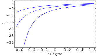
Figure 1: (color online) A plot of the bound state energy $E$(dimension $length^{-2}$) as a function of the self-adjoint extension parameter $\Sigma$. From top to bottom $\eta=0.7,0.6,0.5$ respectively.

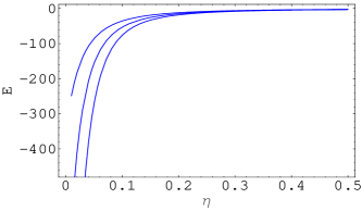
Figure 2: (color online) A plot of the bound state energy $E$(dimension $length^{-2}$) as a function of the coupling constant $\eta\neq 0$. From top to bottom $\Sigma=\pi/6,\pi/7,\pi/8$ respectively.

III SAE of the radial Hamiltonian

We need to construct a domain for our Hamiltonian $H_{\rho}$, because otherwise the Hamiltonian does not have any meaning. $H_{\rho}$ is formally self-adjoint, but formal self-adjointness of an operator does not mean that it is self-adjoint. To start with, we search for a very restricted domain $\mathcal{D}(H_{\rho})$ so that $H_{\rho}$ is symmetric (or hermitian) in that domain. $H_{\rho}$ can be made symmetric for $\forall\psi_{1},\psi_{2}\in\mathcal{D}(H_{\rho})$, if the R.H.S of

$$(H_{\rho}\psi_{1}(\rho),\psi_{2}(\rho))-(\psi_{1}(\rho),H_{\rho}\psi_{2}(\rho))=\Delta(\infty)-\Delta(0),$$

where $\Delta(r)=\psi_{1}(\rho)\dot{\psi}_{2}(\rho)-\dot{\psi}_{1}(\rho)\psi_{2}(\rho)$, is zero. The asymptotic limit of the functions $\psi_{1},\psi_{2}$ are assumed to fall to zero, so we get $\Delta(\infty)=0$. The condition for symmetric Hamiltonian thus reduces to $\Delta(0)=0$ and it can be easily achieved if the elements of $\mathcal{D}(H_{\rho})$ and their derivatives with respective to $\rho$ becomes zero at origin. We then need to get the domain $\mathcal{D}(H^{*}_{\rho})$ of the operator $H^{*}_{\rho}$ (this operator is adjoint to the Hamiltonian $H_{\rho}$). Since $H_{\rho}$ is formally self-adjoint, its adjoint $H^{*}_{\rho}$ should have the same form and the elements $\xi\in\mathcal{D}(H^{*}_{\rho})$ can now be found from

$$(H^{*}_{\rho}\xi(\rho),\psi(\rho))-(\xi(\rho),H_{\rho}\psi(\rho))=0,\forall\psi(\rho)\in\mathcal{D}(H_{\rho}).$$ (4)

We see that the elements $\psi(\rho)$ ($\psi(\rho)\in\mathcal{D}(H_{\rho})$) are so restricted that no restriction on the elements $\xi(\rho)$ ($\xi(\rho)\in\mathcal{D}(H^{*}_{\rho})$) are required in order to satisfy (4). Since the two domains $\mathcal{D}(H_{\rho})$ and $\mathcal{D}(H^{*}_{\rho})$ are not equal, i.e., $\mathcal{D}(H_{\rho})\neq\mathcal{D}(H^{*}_{\rho})$, the operator $H_{\rho}$ is not self-adjoint in the domain $\mathcal{D}(H_{\rho})$. To find out the possible SAE we follow the well known von Neumann’s method. We have to find out the square integrable solutions of $H_{\rho}^{*}\phi_{\pm}=\pm i\phi_{\pm}$. The square integrable solutions can be written in terms of Hankel functions ($H^{(1)},H^{(2)}$) abr as $\phi_{+}(\rho)=\sqrt{\rho}H^{(1)}_{\eta}(\rho e^{i\frac{\pi}{4}})$ and $\phi_{-}(\rho)=\sqrt{\rho}H^{(2)}_{\eta}(\rho e^{-i\frac{\pi}{4}})$. These solutions are square integrable at origin for $\eta^{2}\in[0,1)$. This can be checked from the short distance behavior

$$\lim_{\rho\to 0}|\phi_{\pm}(\rho)|^{2}=()\rho+()\rho^{2\eta+1}+()\rho^{-2\eta+1}\,,$$ (5)

where $()$s are constants, which are unimportant for this purpose. It can also be checked from (5) that for $\eta^{2}\geq 1$ $\phi_{\pm}(\rho)$ are not square integrable at the origin. In this case $H_{\rho}$ is essentially self-adjoint. Our next task is to get a SAE for $\eta^{2}\in[0,1)$ and it will be characterized by a single parameter $\Sigma$. The Hamiltonian $H_{\rho}$ will now be self adjoint over the newly defined domain $\mathcal{D}_{\Sigma}(H_{\rho})\equiv D(H_{\rho})+\phi_{+}(\rho)+\exp(i\Sigma)\phi_{-}(\rho)$, where $\Sigma\in R$ (mod $2\pi$) reed . Using $\mathcal{D}_{\Sigma}(H_{\rho})$ we have to calculate the bound state solutions. The bound state eigenfunction of (2) is

$$R(\rho) \equiv \sqrt{\rho}H^{(1)}_{\eta}(\sqrt{E}\rho),~{}~{}~{}~{}~{}~{}~{}~{}~{}\eta\neq 0$$ (6)

$$\equiv \sqrt{-2E\rho}K_{0}\left(\sqrt{-E}\rho\right),\eta=0$$

where $K_{0}$ is the modified Bessel function abr . Note that for $\eta=0$ we just mention the results, but the calculations should be done separately to get the results. The bound state eigenvalue $E$ of (2) can be calculated from the relation

$$\lim_{\rho\to 0}R(\rho)=\lim_{\rho\to 0}\left(\phi_{+}(\rho)+\exp(i\Sigma)\phi_{-}(\rho)\right)\,.$$ (7)

Equating the coefficients of $\rho^{\eta+1/2}$ and $\rho^{-\eta+1/2}$ from both sides of (7) and comparing between them we get a single bound state energy

$$E = -\sqrt[\eta]{\cos(\pi\eta/2)+\cot(\Sigma/2+\pi\eta/4)\sin(\pi\eta/2)},\eta\neq 0$$ (8)

$$= -{\exp}\left[(\pi/2){\cot}(\Sigma/2)\right],~{}~{}~{}~{}~{}~{}~{}~{}~{}~{}~{}~{}~{}~{}~{}~{}~{}~{}~{}~{}~{}~{}~{}~{}\eta=0$$

for a fixed value of $\eta^{2}$. Note that only those values of $\Sigma$ give bound state solution for which the quantity under third bracket in (8) is positive. Since for different values of the SAE parameter $\Sigma$ we get different boundary conditions and thus different systems, this can be recognized as inequivalent quantization.

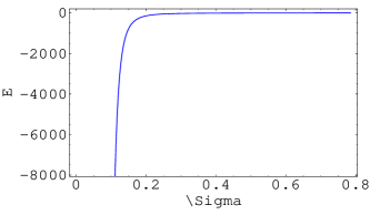
Figure 3: (color online) A plot of the bound state energy $E$(dimension $length^{-2}$) as a function of the self-adjoint extension parameter $\Sigma$ for $\eta=0$.

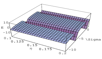
Figure 6: (color online) A 3-dimensional plot of the eigenvalue $E$ as a function of the parameter $\eta$ and $\Sigma$.

In FIG. 1, the bound state energy $E$ has been plotted as a function of the self-adjoint extension parameter $\Sigma$ for three different values of the coupling constant $\eta\neq 0$. In FIG. 2, the same bound state energy has been plotted as a function of the coupling constant $\eta$ for three different values of the self-adjoint extension parameter $\Sigma$. Since, for $\eta=0$, the expression for the eigenvalue $E$ is different, it has thus been plotted in FIG. 3 separately. The 3-dimensional plot of the eigenvalue $E$ as a function of the two parameters $\eta$ and $\sigma$ is shown in FIG. 6.

IV Re-normalization in NA system

For strong attractive ($\eta^{2}<0$) inverse square potential, the usual analysis of the NA system will give a tower of spectrum case with ground state being $-\infty$. Even the self-adjointness technique feher also gives the ground state to be -ve infinity. This implies that the system will collapse if $\eta^{2}<0$. But re-normalization technique rajeev ; hor ; bawin ; braaten has a remedy for this problem to give a finite ground state, thus making the problem physically realizable. In re-normalization technique, the divergent Hamiltonian is regularized with an ultraviolet cut off $\rho=\Theta$, for example consider an infinite barrier regularized potential

$$V(\rho) = \infty\,,~{}~{}~{}~{}~{}~{}~{}\mbox{for}~{}~{}\rho<\Theta$$ (9)

$$= \frac{\mbox{g}(\Theta)}{\rho^{2}}\,,~{}~{}~{}\mbox{for}~{}~{}\rho\geq\Theta$$

where now the coupling constant depends on the ultraviolet cut off, $\mbox{g}(\Theta)=(\eta^{2}(\Theta)-1/4)$. The ultraviolet cut off allows the system to sustain a well defined bound state. This can be understood form the regularized time independent Schrödinger equation

$$\left(H_{\rho}(\Theta)-E(\Theta)\right)R(\rho,\Theta)=0\,,~{}\mbox{for}~{}\rho\geq\Theta$$ (10)

with the boundary condition that $R(\rho=\Theta,\Theta)=0$. The dependence of the coupling constant $\eta(\Theta)$ on the ultraviolet cutoff $\Theta$ is encoded in the relation

$$\frac{dH_{\rho}(\Theta)}{d\Theta}=\left[\frac{d}{d\Theta},H_{\rho}(\Theta)\right]\,.$$ (11)

The relation of the coupling constant with the ultraviolet cut off can be obtained from (11) to be

$$\frac{d\eta^{2}(\Theta)}{d\Theta}=\rho^{2}\left[\frac{d}{d\Theta},H_{\rho}(\Theta)\right]\,.$$ (12)

The coupling $\eta(\Theta)$ goes to zero in the limit $\Theta\to 0$ rajeev . Thus $\eta=0$ is the ultraviolet stable point for the system.

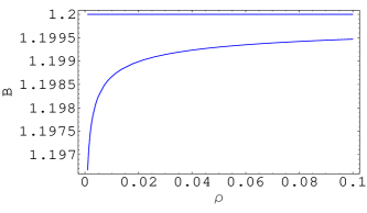
Figure 4: (color online) A plot of the absolute value of the quantity $B=\frac{|\lim_{\rho\to 0}\Lambda\phi(\rho)|}{|\lim_{\rho\to 0}\phi(\rho)|}$ as a function of $\rho$ for $\eta=0.2$. The straight line corresponds to $\Sigma=-\frac{\pi}{10}$ and curve line corresponds to $\Sigma=-1.001.\frac{\pi}{10}$. The point $(\eta,\Sigma)\equiv(0.2,-\frac{\pi}{4})$ associated with the straight line is the point in the $\eta,\Sigma$ parametric space where scaling is unbroken on the other hand at the point $(\eta,\Sigma)\equiv(0.2,-1.001.\frac{\pi}{4})$ associated with the curve line, scale symmetry is broken.

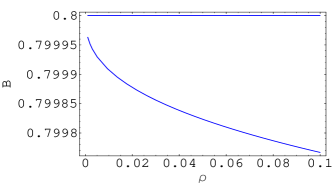
Figure 5: (color online) A plot of the absolute value of the quantity $B=\frac{|\lim_{\rho\to 0}\Lambda\phi(\rho)|}{|\lim_{\rho\to 0}\phi(\rho)|}$ as a function of $\rho$ for $\eta=0.2$. The straight line corresponds to $\Sigma=-\frac{3\pi}{10}$ and curve line corresponds to $\Sigma=-1.001.\frac{3\pi}{10}$. The point $(\eta,\Sigma)\equiv(0.2,-\frac{3\pi}{4})$ associated with the straight line is the point in the $\eta,\Sigma$ parametric space where scaling is unbroken on the other hand at the point $(\eta,\Sigma)\equiv(0.2,-1.001.\frac{3\pi}{4})$ associated with the curve line, scale symmetry is broken.

V Scaling anomaly of NA system

We now discuss scaling symmetry and its anomaly alfaro ; esteve ; gozzi ; gozzi1 ; govinda ; gino for the full $3$-dimensional problem of a neutral atom in the magnetic field of a ferromagnetic wire. Classically the action constructed from the Hamiltonian $H={\bm{p}}^{2}/2\mu-\bm{\mu}.\bm{B}$ is scale invariant under the scale transformation $\bm{r}\to\varrho\bm{r}$ and $t\to\varrho^{2}t$, where $\bm{r}=x\hat{i}+y\hat{j}+z\hat{k}$, $\varrho$ is the scale factor, $t$ is the time. The Hamiltonian transforms as $H\to(1/\varrho^{2})H$ under the scale transformation. Lagrangian constructed from this Hamiltonian $H$ also transforms in the same way $L\to(1/\varrho^{2})L$. So the action of our system is evidently scale invariant as stated above. The consequence of scale invariance is that the system should not have any bound state. Because, the presence of bound state energy would provide a scale govinda for the system and consequently scale invariance will break down.

We have seen in our previous section that after inequivalent quantization of the Hamiltonian, the use of nontrivial boundary condition gives a single bound state in the interval $\eta^{2}\in[0,1)$ for the $2$-dimensional problem ($x$-$y$ plane). This single bound state is however a characteristic feature of the of the inverse square potential and has been obtained in literature giri1 ; giri ; giri3 ; giri4 ; alfaro ; esteve ; gozzi ; gozzi1 ; govinda ; gino ; cabo before. Note that the motion along $z$ direction is still given by a free particle solution $e^{ikz}$. Bound state energy given by (8) provides a scale for the $2$-dimensional the system, leading to “partial scaling anomaly”. We use the term “partial scaling anomaly”, because in the $z$ direction scaling symmetry is still restored even after quantization. This situation happens in other cylindrically symmetric systems also, for example the motion of a charged particle or a dipole in cosmic string background giri1 ; giri show partial scale symmetry breaking. Quantum mechanically scaling transformation is associated with a scaling operator alfaro ; govinda $\Lambda=-\frac{i}{2}(\rho\frac{d}{d\rho}+\frac{d}{d\rho}\rho)$. For a generic element $\phi(\rho)\in\mathcal{D}_{\Sigma}(H_{\rho})$ and for $\Sigma\neq-\frac{\eta\pi}{2}$ or $\neq-\frac{3\eta\pi}{2}$, $\Lambda\phi(\rho)\notin\mathcal{D}_{\Sigma}(H_{\rho})$. This can be checked from the relation

$$\lim_{\rho\to 0}\Lambda\phi(\rho)\neq C\lim_{\rho\to 0}\phi(\rho),~{}\mbox{for}~{}\eta\neq 0$$ (13)

where $C$ is any complex number. Since the action of $\Lambda$ on the domain $\mathcal{D}_{\Sigma}(H_{\rho})$ does not keep the domain invariant, scaling symmetry is broken govinda . But it can be shown that for $\Sigma=-\frac{\eta\pi}{2}$ and $-\frac{3\eta\pi}{2}$, scaling symmetry is restored kumar1 ; kumar2 ; kumar3 even after quantization. In this case

$$\Lambda\phi(\rho)\in\mathcal{D}_{\Sigma}(H_{\rho}),~{}~{}\mbox{for}~{}~{}\eta\neq 0$$ (14)

For more clarity on scale symmetry and its anomalous breaking we plot the ratio of $|\lim_{\rho\to 0}\Lambda\phi(\rho)|$ to $|\lim_{\rho\to 0}\phi(\rho)|$ as a function of the radial variable $\rho$ for $\eta=0.2$. Note that for $\eta=0.2$, scale symmetry is restored for $\Sigma=-\frac{\pi}{10}$ and $\Sigma=-\frac{3\pi}{10}$ respectively. The straight line in FIG. 4 corresponds to $\Sigma=-\frac{\pi}{10}$ and straight line in FIG. 5 corresponds to $\Sigma=-\frac{3\pi}{10}$. On the other hand the scaling anomaly is displayed by the two curved line in FIG. 4 and FIG. 5 respectively. One can similarly discuss the scaling anomaly for the $\eta=0$ case from its bound state solution and its domain. It can also be noted that the two scaling symmetry points is associated with two extreme points on the energy scale for bound state of the system, one is at $E=0$ and other is at $E=\infty$.

VI Conclusion

In literature tka it is usually said that the neutral atom would not have any stable bound state under the magnetic field of a ferromagnetic wire and depending on the coupling constant $\eta^{2}$, it will either be unbounded (for $\eta^{2}>0$) or fall into the singularity (for $\eta^{2}<0$). In our work we have shown that the assumption in the literature is not true, if we allow nontrivial boundary condition to hold for the system, contrary to the result of the previous literature tka , where usual boundary condition has been considered. It is in fact possible to form stable bound state for the $2$-dimensional problem in the field of a ferromagnetic wire. The dynamics along $z$ direction is given by free state solution due to cylindrical symmetry of the system. We have also shown that scaling symmetry is partially violated due to nontrivial quantization of the system. Scaling symmetry in $z$ direction still survives even after quantization, so there is no bound state solution in $z$ coordinate. On the other hand on $x$-$y$ plane, scaling symmetry is broken due to quantization, leading to bound state solution. For strong coupling region, $\eta^{2}<0$, re-normalization technique can be used to find a physical bound state solution. $\eta=0$ is then identified as the ultraviolet stable fixed point for the neutral atom system.

References

- (1) V. M. Tkachuk, Phys. Rev. A60, 4715 (1999).
- (2) L. D. Landau and E. M. Lifshitz, Quantum Mechanics, (Pergamon Press, London, 1959).
- (3) M. Reed and B. Simon, Fourier Analysis, Self-Adjointness ( New York :Academic, 1975 ).
- (4) P. R. Giri, arXiv:0704.1725v2 [hep-th].
- (5) P. R. Giri, Phys. Rev. A76, 012114 (2007).
- (6) H. E. Camblong, L. N. Epele, H. Fanchiotti and C. A. G. Canal, Phys. Rev. Lett. 87 220402 (2001); H. E. Camblong, C. R. Ordonez, Phys. Rev. D68, 125013 (2003).
- (7) P. R. Giri, K. S. Gupta, S. Meljanac and A. Samsarov, hep-th/0703121.
- (8) B. Basu-Mallick, Pijush K. Ghosh and Kumar S. Gupta, Nucl. Phys. B659, 437 (2003).
- (9) B. Basu-Mallick and Kumar S. Gupta, Phys. Lett. A292, 36 (2001).
- (10) B. Basu-Mallick, Pijush K. Ghosh and Kumar S. Gupta, Phys. Lett. A311, 87 (2003).
- (11) Kumar S. Gupta, Mod. Phys. Lett. A18, 2355 (2003).
- (12) D. Birmingham, Kumar S. Gupta and Siddhartha Sen, Phys. Lett. B505, 191 (2001); Kumar S. Gupta and Siddhartha Sen, Phys. Lett. B526, 121 (2002).
- (13) S. Meljanac, A. Samsarov, B. Basu-Mallick and Kumar S. Gupta, Eur. Phys. J. C49, 875 (2007).
- (14) P. R. Giri, arXiv:0708.0707v1 [hep-th].
- (15) L. Feher, I. Tsutsui, T. Fulop, Nucl.Phys. B715, 713 (2005).
- (16) P. R. Giri, arXiv:0706.2945v1 [cond-mat.mtrl-sci].
- (17) T. Ristroph, A. Goodsell, J. A. Golovchenko and L. V. Hau, Phys. Rev. Lett. 94, 066102 (2005).
- (18) M. Abromowitz, I. A. Stegun, Handbook of Mathematical Functions (Dover, New York, 1970).
- (19) K. M. Case, Phys. Rev. 80, 797 (1950).
- (20) K. S. Gupta and S. G. Rajeev, Phys. Rev. D48, 5940 (1993).
- (21) H. E. Camblong, L. N. Epele, H. Fanchiotti and C. A. Garcia Canal, Phys. Rev. Lett. 85, 1590 (2000).
- (22) M. Bawin and S. A. Coon, Phys. Rev. A76, 042712 (2003).
- (23) E. Braaten and D. Phillips, Phys. Rev. A70, (2004).
- (24) V. de Alfaro, S. Fubini and G. furlan, Nuovo Cimento 34A, 569 (1976).
- (25) J. G. Esteve, Phys. Rev. D66, 125013 (2002).
- (26) E. Gozzi and D. Mauro, Phys. Lett. A345, 273 (2005).
- (27) E. Gozzi and D. Mauro, J. Phys. A39, 3411 (2006).
- (28) T. R. Govindarajan, V. suneeta and S. Vaidya, Nucl. Phys. B583, 291 (2000).
- (29) G. N. J. Ananos, H. E. Camblong, C. R. Ordonez, Phys. Rev. D68, 025006 (2003).
- (30) A. Cabo, J. L. Lucio and H. Mercado, Am. J. Phys. 66, 240 (1998).