Experimental joint signal-idler quasi-distributions and photon-number statistics for mesoscopic twin beams

Abstract

Joint signal-idler photoelectron distributions of twin beams containing several tens of photons per mode have been measured recently. Exploiting a microscopic quantum theory for joint quasi-distributions in parametric down-conversion developed earlier we characterize properties of twin beams in terms of quasi-distributions using experimental data. Negative values as well as oscillating behaviour in quantum region are characteristic for the subsequently determined joint signal-idler quasi-distributions of integrated intensities. Also the conditional and difference photon-number distributions are shown to be sub-Poissonian and sub-shot-noise, respectively.

I Introduction

The process of spontaneous parametric down-conversion Walls1994 ; Mandel1995 ; Perina1994 is one of the fundamental nonlinear quantum processes that can be understood in terms of created and annihilated photon pairs. This highly nonclassical origin of the generated optical fields is responsible for their unusual properties. They have occurred to be extraordinarily useful in verification of fundamental laws of quantum mechanics using tests of Bell inequalities Perina1994 , generation of Greenberger-Horne-Zeilinger states Bouwmeester1999 , demonstration of quantum teleportation Bouwmeester1997 , quantum cryptography Lutkenhaus2000 , dense coding, and many other ‘quantum protocols’ Bouwmeester2000 . Fields composed of photon pairs have already found applications, e.g. in quantum cryptography Lutkenhaus2000 or metrology Migdal1999 . Description of this process has been elaborated from several points of view for beams containing just one photon pair with a low probability Keller1997 ; PerinaJr1999 ; DiGiuseppe1997 ; Grice1998 ; PerinaJr2006 as well as for beams in which many photon pairs occur Nagasako2002 . Also stimulated emission of photon pairs has been investigated Lamas-Linares2001 ; DeMartini2002 ; Pellicia2003 .

Recent experiments Agliati2005 ; Haderka2005 ; Haderka2005a ; Bondani2007 ; Paleari2004 (and references therein) have provided experimental joint signal-idler photoelectron distributions of twin beams containing up to several thousands of photon pairs. Extremely sensitive photodiodes, special single-photon avalanche photodiodes Kim1999 , super-conducting bolometers Miller2003 , time-multiplexed fiber-optics detection loops Haderka2004 ; Rehacek2003 ; Achilles2004 ; Fitch2003 , intensified CCD cameras Jost1998 ; Haderka2005 , or methods measuring attenuated beams Zambra2005 ; Zambra2006 are available at present as detection devices able to resolve photon numbers. Also homodyne detection has been applied to determine intensity correlations of twin beams Vasilyev2000 ; Zhang2002 . These advances in experimental techniques have stimulated the development of a detailed microscopic theory able to describe such beams and give an insight into their physical properties. A theory based on multi-mode description of the generated fields has been elaborated both for spontaneous Perina2005 as well as stimulated processes Perina2006 . This theory allows one to determine the joint signal-idler quasi-distribution of integrated intensities from measured joint signal-idler photoelectron distributions. Considering phases of multi-mode fields generated in this spontaneous process to be completely random, the joint signal-idler quasi-distribution of integrated intensities gives us a complete description of the generated twin beams. As a consequence of pairwise emission the quasi-distribution of integrated intensities has a typical shape and attains negative values in some regions. This quasi-distribution has been already experimentally reached Haderka2005 ; Haderka2005a for twin beams containing up to several tens of photon pairs but with mean numbers of photons per mode being just a fraction of one. Here, we report on experimental determination of the joint signal-idler quasi-distribution of integrated intensities for twin beams containing several tens of photons per mode. Such system may be considered as mesoscopic and this makes its properties extraordinarily interesting for an investigation.

Photon-number distributions and quasi-distributions of integrated intensities provided by theory are contained in Sec. II. Section III is devoted to the analysis of experimental data. Conclusions are drawn in Sec. IV.

II Photon-number distributions and quasi-distributions of integrated intensities

In the experiment, whose layout is sketched in Fig. 1 (for details, see Bondani2007 ), the third harmonic field (wavelength 349 nm and time duration 4.45 ps) of an amplified mode-locked Nd:YLF laser with repetition rate of 500 Hz (High Q Laser Production, Hohenems, Austria) is used to pump parametric down-conversion in a BBO crystal (Fujian Castech Crystals, Fuzhou, China) cut for type-I interaction. The down-converted beams at wavelengths of 632.8 and 778.2 nm are selected by two 100 $\mu$m diameter apertures and directed into two amplified pin photodiodes (S5973-02 and S3883, Hamamatsu Photonics K.K., Japan) using lenses of appropriate focal lengths (see Fig. 1). The output current pulses are digitized and processed by a computer. The overall detection quantum efficiencies, $\eta$, are 55 % for both arms. First ($\langle m\rangle$) and second ($\langle m^{2}\rangle$) moments of photoelectron distributions for both signal and idler beams as well as correlation of photoelectron numbers in the signal and idler beams are obtained experimentally. Additive noise present during detection can be measured separately and subtracted from the measured data. The measured moments of photoelectron numbers can be corrected also for the overall quantum efficiency and we then obtain the moments for photons. Symbol $\langle n_{1}\rangle$ ($\langle n_{2}\rangle$) means mean photon number in signal (idler) field, $\langle n_{1}^{2}\rangle$ ($\langle n_{2}^{2}\rangle$) denotes the second moment of signal- (idler-) field photon-number distribution, and $\langle n_{1}n_{2}\rangle$ gives correlations in the number of signal and idler photons. We note that moments of photon-number distributions are obtained using the relations:

$$\langle n_{i}\rangle = \langle m_{i}\rangle/\eta,$$

$$\langle n_{i}^{2}\rangle = \langle m_{i}^{2}\rangle/\eta^{2}-(1-\eta)\langle m_{i}\rangle/\eta^{2},\hskip 14.22636pti=1,2,$$

$$\langle n_{1}n_{2}\rangle = \langle m_{1}m_{2}\rangle/\eta^{2}.$$ (1)

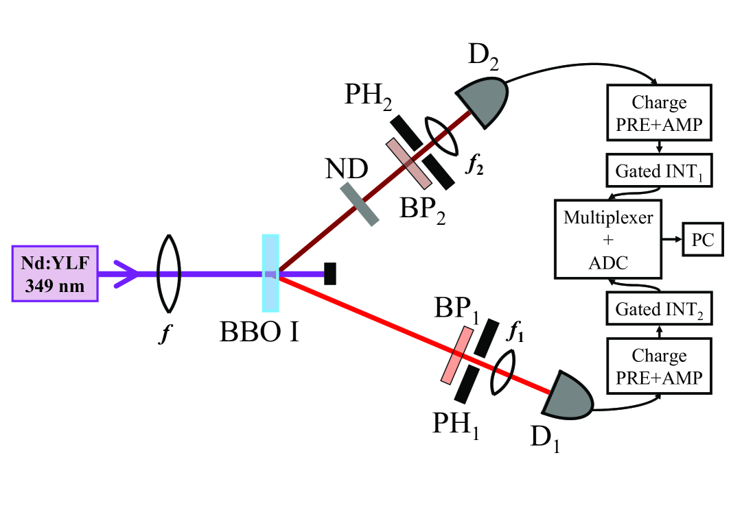
Figure 1: (Color online) Sketch of the experimental setup. Nd:YLF, amplified ps-pulsed laser source; BBO I, nonlinear crystal; $f$, $f_{1,2}$, lenses; PH_1,2, 100 $\mu$m diameter pin-holes; D_1,2, pin detectors; BP_1,2, band-pass filters; ND, adjustable neutral-density filter. The boxes on the right-hand side indicate the parts of the signal amplification and acquisition chains.

Moments of integrated intensities can be directly derived from moments of photon numbers:

$$\langle W_{i}\rangle = \langle n_{i}\rangle,$$

$$\langle W_{i}^{2}\rangle = \langle n_{i}^{2}\rangle-\langle n_{i}\rangle,\hskip 5.69054pti=1,2,$$

$$\langle W_{1}W_{2}\rangle = \langle n_{1}n_{2}\rangle.$$ (2)

Multi-mode theory of down-conversion developed in Perina2005 using a generalized superposition of signal and noise provides the following relations between the above mentioned experimental quantities and quantum noise coefficients $B_{1}$, $B_{2}$, $D_{12}$, and the number $M$ of modes:

$$\langle W_{i}\rangle = MB_{i},$$

$$\langle(\Delta W_{i})^{2}\rangle = MB_{i}^{2},\hskip 5.69054pti=1,2,$$

$$\langle\Delta W_{1}\Delta W_{2}\rangle = M|D_{12}|^{2}.$$ (3)

The coefficient $B_{i}$ gives mean number of photons in mode $i$ and $D_{12}$ characterizes mutual correlations between the signal and idler fields. Inverting relations in Eqs. (3) we arrive at the expressions for parameters $B_{1}$, $B_{2}$, $M$, and $D_{12}$:

$$B_{i} = \langle(\Delta W_{i})^{2}\rangle/\langle W_{i}\rangle,$$

$$M_{i} = \langle W_{i}\rangle^{2}/\langle(\Delta W_{i})^{2}\rangle,\hskip 5.69054pti=1,2,$$

$$|D_{12}| = \sqrt{\langle\Delta W_{1}\Delta W_{2}\rangle/M}.$$ (4)

As follows from Eqs. (4), the number $M$ of modes can be determined from experimental data measured either in the signal or idler field. This means that the experimental data give two numbers $M_{1}$ and $M_{2}$ of modes as a consequence of non-perfect alignment of the setup and non-perfect exclusion of noise from the data. On the other hand, there occurs only one number $M$ of modes (number of degrees of freedom) in the theory Perina2005 as it assumes that all pairs of mutually entangled signal- and idler-field modes are detected at both detectors. Precise fulfillment of this requirement can hardly be reached under real experimental conditions. However, experimental data with $M_{1}\approx M_{2}$ can be obtained.

Joint signal-idler photon-number distribution $p(n_{1},n_{2})$ for multi-thermal field with $M$ degrees of freedom and composed of photon pairs can be derived in the form Perina2005 :

$$p(n_{1},n_{2}) = \frac{1}{\Gamma(M)}\frac{(-K)^{n_{2}}(B_{1}+K)^{n_{1}-n_{2}}}{(1+B_{1}+B_{2}+K)^{n_{1}+M}}$$ (5)

$$\mbox{}\times\sum_{r={\rm max}(0,n_{2}-n_{1})}^{n_{2}}\frac{\Gamma(n_{1}+M+r)}{r!(n_{2}-r)!(n_{1}-n_{2}+r)!}$$

$$\mbox{}\times\frac{[(B_{1}+K)(B_{2}+K)]^{r}}{(-K)^{r}(1+B_{1}+B_{2}+K)^{r}}.$$

Determinant $K$ introduced in Eq. (5) and given by the expression

$$K=B_{1}B_{2}-|D_{12}|^{2}$$ (6)

is crucial for the judgement of classicality of a field. Negative values of the determinant $K$ mean that a given field cannot be described classically as in case of the considered field composed of photon pairs. In Eq. (5), the quantities $B_{1}+K$ and $B_{2}+K$ cannot be negative and can be considered as characteristics of fictitious noise present in the signal and idler fields, respectively. The theory for an ideal lossless case gives $K=-B_{1}=-B_{2}$ together with the joint photon-number distribution $p(n_{1},n_{2})$ in the form of diagonal Mandel-Rice distribution. On the other hand inclusion of losses and external noise results in non-diagonal photon-number distribution $p(n_{1},n_{2})$ as a consequence of the fact that not all detected photons are paired. We note that pairing of photons leads to higher values of elements $p(n_{1},n_{2})$ of the joint signal-idler photon-number distribution around the diagonal $n_{1}=n_{2}$ that violate a classical inequality derived in Haderka2005 .

A compound Mandel-Rice formula gives the joint signal-idler photon-number distribution $p(n_{1},n_{2})$ at the border between the classical and nonclassical characters of the field ($K=0$):

$$p(n_{1},n_{2})=\frac{\Gamma(n_{1}+n_{2}+M)B_{1}^{n_{1}}B_{2}^{n_{2}}}{\Gamma(M)n_{1}!\,n_{2}!\,(1+B_{1}+B_{2})^{n_{1}+n_{2}+M}}.$$ (7)

If the number $M$ of modes is large compared to mean values $\langle n_{1}\rangle$ and $\langle n_{2}\rangle$ (i.e. for $B_{1}$, $B_{2}$, and $|D_{12}|$ being small) the expression in Eq. (7) can roughly be approximated by a product of two Poissonian distributions. If $K>0$ or $K<0$, weak classical or quantum fluctuations remain in this Poisson limit of a large number $M$ of modes, as follows from the normal generating function Perina2005 in the form $G(\lambda_{1},\lambda_{2})\approx\exp(-\lambda_{1}\langle n_{1}\rangle-\lambda_{2}\langle n_{2}\rangle+\lambda_{1}\lambda_{2}M|D_{12}|^{2})$ valid in this approximation. Thus there are always mode correlations in agreement with the third formula in Eq. (3).

Declination from an ideal diagonal distribution $p(n_{1},n_{2})$ caused by losses can be characterized using conditional idler-field photon-number distribution $p_{c,2}(n_{2};n_{1})$ measured under the condition of detected $n_{1}$ signal photons and determined along the formula:

$$p_{c,2}(n_{2};n_{1})=p(n_{1},n_{2})/\sum_{k=0}^{\infty}p(n_{1},k).$$ (8)

Substitution of Eq. (5) in Eq. (8) leads to the conditional idler-field photon-number distribution $p_{c,2}$ with Fano factor $F_{c,2}$:

$$F_{c,2}(n_{1}) = 1$$ (9)

$$\mbox{}+\frac{(1+M/n_{1})[(B_{2}+K)/(1+B_{1})]^{2}-(K/B_{1})^{2}}{(1+M/n_{1})(B_{2}+K)/(1+B_{1})-K/B_{1}}$$

$$\approx 1+K/B_{1}.$$

As an approximate expression for the Fano factor $F_{c,2}$ in Eq. (9) (valid for $K\approx-B_{2}$ ) indicates negative values of the determinant $K$ are necessary to observe sub-Poissonian conditional photon-number distributions. Sub-Poissonian conditional distribution $p_{c,2}$ emerges from the formula in Eq. (5) that is a sum of positive terms in this case. For the ideal lossless case, $K=-B_{1}=-B_{2}$ holds and the Fano factor $F_{c,2}$ equals 0. On the other hand, positive values of the determinant $K$ mean that the sum in Eq. (5) contains large terms with alternating sings (this may lead to numerical errors in summation) and so the conditional distribution $p_{c,2}$ is super-Poissonian. For instance, for $K$ small compared to $B_{1}$, $F_{c,2}=1+(B_{2}+K)/(1+B_{1})$. We note that, in this approximation, the value of Fano factor $F_{c,2}$ equals the value of coefficient $R$ quantifying sub-shot-noise correlations and being defined in Eq. (11) below.

Pairing of photons in the detected signal and idler fields leads to narrowing of distribution $p_{-}$ of the difference $n_{1}-n_{2}$ of signal- and idler-field photon numbers:

$$p_{-}(n)=\sum_{n_{1},n_{2}=0}^{\infty}\delta_{n,n_{1}-n_{2}}p(n_{1},n_{2})$$ (10)

and $\delta$ denotes Kronecker symbol. If variance of the difference $n_{1}-n_{2}$ of signal- and idler-field photon numbers is less than the sum of mean photon numbers in the signal and idler fields we speak about sub-shot-noise correlations and characterize them by coefficient $R$ Bondani2007 :

$$R=\frac{\langle[\Delta(n_{1}-n_{2})]^{2}\rangle}{\langle n_{1}\rangle+\langle n_{2}\rangle}<1.$$ (11)

Joint signal-idler photon-number distribution $p(n_{1},n_{2})$ and joint signal-idler quasi-distribution $P_{1}(W_{1},W_{2})$ of integrated intensities belonging to normally-ordered operators are connected through Mandel’s detection equation Perina1994 ; Saleh1978 :

$$p(n_{1},n_{2}) = \frac{1}{n_{1}!\,n_{2}!}\int_{0}^{\infty}dW_{1}\,\int_{0}^{\infty}dW_{2}\,W_{1}^{n_{1}}W_{2}^{n_{2}}$$ (12)

$$\mbox{}\times\exp(-W_{1}-W_{2})P_{1}(W_{1},W_{2}).$$

Relation in Eq. (12) can be generalized to an arbitrary ordering of field operators Perina1994 ; Perina2005 and can be inverted in terms of series of Laguerre polynomials. Range of convergence of these series is determined under the condition $s\leq s_{\rm th}$ where $s_{th}$ is given in Eq. (15) later. These series define quasi-distributions for $s>s_{\rm th}$.

Provided that an $s$-ordered determinant $K_{s}$, $K_{s}=B_{1s}B_{2s}-|D_{12}|^{2}$ ($B_{i,s}=B_{i}+(1-s)/2$, $i=1,2$), is positive the $s$-ordered joint signal-idler quasi-distribution $P_{s}(W_{1},W_{2})$ of integrated intensities exists as an ordinary function Perina2005 which cannot take on negative values:

$$P_{s}(W_{1},W_{2}) = \frac{1}{\Gamma(M)K_{s}^{M}}\left(\frac{K_{s}^{2}W_{1}W_{2}}{|D_{12}|^{2}}\right)^{(M-1)/2}$$ (13)

$$\mbox{}\times\exp\left[-\frac{(B_{2s}W_{1}/B_{1s}+W_{2})B_{1s}}{K_{s}}\right]$$

$$\mbox{}\times I_{M-1}\left(2\sqrt{\frac{|D_{12}|^{2}W_{1}W_{2}}{K_{s}^{2}}}\right).$$

Symbol $I_{M}$ denotes modified Bessel function and $\Gamma$ stands for $\Gamma$-function.

If the $s$-ordered determinant $K_{s}$ is negative, the joint signal-idler quasi-distribution $P_{s}$ of integrated intensities exists in general as a generalized function that can be negative or even have singularities. It can be approximated by the following formula Perina2005 :

$$P_{s}(W_{1},W_{2}) \approx \frac{A(W_{1}W_{2})^{(M-1)/2}}{\pi\Gamma(M)(B_{1s}B_{2s})^{M/2}}\exp\left(-\frac{W_{1}}{2B_{1s}}-\frac{W_{2}}{2B_{2s}}\right)$$ (14)

$$\mbox{}\times\rm{sinc}\left[A\left(\frac{B_{2s}}{B_{1s}}W_{1}-W_{2}\right)\right];$$

${\rm sinc}(x)=\sin(x)/x$. Oscillating behaviour is typical for the quasi-distribution $P_{s}$ written in Eq. (14).

There exists a threshold value $s_{\rm th}$ of the ordering parameter $s$ for given values of parameters $B_{1}$, $B_{2}$, and $D_{12}$ determined by the condition $K_{s}=0$:

$$s_{\rm th}=1+B_{1}+B_{2}-\sqrt{(B_{1}+B_{2})^{2}-4K};$$ (15)

$-1\leq s_{\rm th}\leq 1$. Quasi-distributions $P_{s}$ for $s\leq s_{\rm th}$ are ordinary functions with non-negative values whereas those for $s>s_{\rm th}$ are generalized functions with negative values and oscillations.

Similarly as for photon numbers we can define quasi-distribution $P_{s,-}$ of the difference $W_{1}-W_{2}$ of signal- and idler-field integrated intensities as a quantity useful for description of photon pairing:

$$P_{s,-}(W) = \int_{0}^{\infty}dW_{1}\,\int_{0}^{\infty}dW_{2}\,$$ (16)

$$\mbox{}\times\delta(W-W_{1}+W_{2})P_{s}(W_{1},W_{2}).$$

Quasi-distribution $P_{s,-}$ oscillates and takes on negative values as a consequence of pairwise character of the detected fields if $s\geq s_{\rm th}$.

There exists relation between variances of the difference $n_{1}-n_{2}$ of signal- and idler-field photon numbers and difference $W_{1}-W_{2}$ of signal- and idler-field integrated intensities:

$$\langle[\Delta(n_{1}-n_{2})]^{2}\rangle=\langle n_{1}\rangle+\langle n_{2}\rangle+\langle[\Delta(W_{1}-W_{2})]^{2}\rangle.$$ (17)

According to Eq. (17) negative values of the quasi-distribution $P_{s,-}$ (as well as these of quasi-distribution $P_{s}$) are necessary to observe sub-shot-noise correlations in signal- and idler-field photon numbers as described by the condition $R<1$ in Eq. (11).

III Experimental distributions

As an example, we analyze the following experimental data appropriate for photons and derived from the experimental data for photoelectrons given in Bondani2007 using relations in Eqs. (1) [$\eta=0.55$]:

$$\langle n_{1}\rangle=959.21, \langle n_{2}\rangle=1078.3,$$

$$\langle n_{1}^{2}\rangle=971829.7, \langle n_{2}^{2}\rangle=1218608,$$

$$\langle n_{1}n_{2}\rangle=1088083.$$ (18)

These data thus characterize photon fields, as they have been obtained after correction for the nonunit detection efficiency. Formulas in Eqs. (2) and (4) then give mean number $B_{1}$ of signal photons per mode, mean number $B_{2}$ of idler photons per mode, number $M_{1}$ of signal-field modes, and number $M_{2}$ of idler-field modes:

$$B_{1}=52.95, B_{2}=50.81,$$

$$M_{1}=18.11, M_{2}=21.22.$$ (19)

Numbers $M_{1}$ and $M_{2}$ of modes given in Eqs. (19) and determined from data characterizing signal ($M_{1}$) and idler ($M_{2}$) fields slightly differ owing to experimental imperfections. That is why we use a mean number $M$ of modes [$M=(M_{1}+M_{2})/2$] and determine the coefficient $D_{12}$ along the relation in Eqs. (4):

$$M=19.66,\hskip 14.22636pt|D_{12}|=52.29.$$ (20)

Determinant $K$ given in Eq. (6) then equals -44.23, i.e. the measured field is nonclassical. Coefficient $R$ defined in Eq. (11) equals 0.19 (-7.2 dB reduction of vacuum fluctuations) and this means that fluctuations in the difference $n_{1}-n_{2}$ of signal and idler photon numbers are below shot-noise level. This also means [see Eq. (17)] that variance $\langle[\Delta(W_{1}-W_{2})]^{2}\rangle$ of the difference of signal- and idler-field integrated intensities is negative ($\langle[\Delta(W_{1}-W_{2})]^{2}\rangle=-1654$). Negative value of this variance is caused by pairwise character of the detected fields, which leads to strong correlations in integrated intensities $W_{1}$ and $W_{2}$. Also the value of covariance $C$ ($C=\langle\Delta n_{1}\Delta n_{2}\rangle/\sqrt{\langle[\Delta n_{1}]^{2}\rangle\langle[\Delta n_{2}]^{2}\rangle}$) of signal $n_{1}$ and idler $n_{2}$ photon numbers close to one ($C=0.997$) is evidence of a strong pairwise character of the detected fields. We note that also a two-mode principal squeeze variance $\lambda$ characterizing phase squeezing and related to one pair of modes can be determined along the formula:

$$\lambda=1+B_{1}+B_{2}-2|D_{12}|.$$ (21)

We arrive at $\lambda=0.18$ using our data in Eq. (21) and so the generated field is also phase squeezed.

The joint signal-idler photon-number distribution $p(n_{1},n_{2})$ determined along the formula in Eq. (5) for values of parameters in Eqs. (19) and (20) is shown in Fig. 2. Strong correlations in signal-field $n_{1}$ and idler-field $n_{2}$ photon numbers are clearly visible. Nonzero elements of the joint photon-number distribution $p(n_{1},n_{2})$ are localized around a line given by the condition $n_{1}\approx n_{2}$ as documented in contour plot in Fig. 2.

Figure 2: Joint signal-idler photon-number distribution $p(n_{1},n_{2})$.

Conditional distributions $p_{c,2}$ of idler-field photon numbers $n_{2}$ conditioned by detection of a given number $n_{1}$ of signal photons defined in Eq. (8) are also sub-Poissonian (see Fig. 3). The greater the value of the number $n_{1}$ of signal photons the smaller the value of Fano factor $F_{c,2}$ given in Eq. (9). If mean numbers $\langle n_{1}\rangle$ and $\langle n_{2}\rangle$ of signal- and idler-field photons are small compared to the number $M$ of modes the joint photon-number distribution $p(n_{1},n_{2})$ behaves like a product of two Poissonian distributions and so $F_{c,2}\approx 1$. Fano factor $F_{c,2}$ reaches its asymptotic value after certain value of the number $n_{1}$ of signal-field photons [see discussion below Eq. (7)].

Figure 3: Fano factor $F_{c,2}$ of the conditional signal-idler photon-number distribution $p_{c,2}$ as a function of the number $n_{1}$ of detected signal photons.

Strong correlations in signal-field $n_{1}$ and idler-field $n_{2}$ photon numbers lead to sub-Poissonian distribution $p_{-}$ of the difference $n_{1}-n_{2}$ of photon numbers defined in Eq. (10) (see Fig. 4).

Figure 4: Distributions $p_{-}(n)$ of the difference $n$ of signal-field ($n_{1}$) and idler-field ($n_{2}$) photon numbers; $n=n_{1}-n_{2}$. Solid curve without symbols characterizes the experimental data. Solid curve with $\circ$ gives the distribution obtained from the joint signal-idler photon-number distribution in the form of product of two independent Poissonian distributions with mean photon-numbers given by experimental data and is shown for comparison.

Joint signal-idler quasi-distributions $P_{s}(W_{1},W_{2})$ of integrated intensities differ qualitatively according to the value of ordering parameter $s$ ($s_{\rm th}=0.15$ for the experimental data). Nonclassical character of the detected fields is smoothed out ($K_{s}=2.66>0$) for the value of $s$ equal to 0.1 as shown in Fig. 5(a). On the other hand, the value of $s$ equal to 0.2 is sufficient to observe quantum features ($K_{s}=-2.53<0$) in the joint signal-idler quasi-distribution $P_{s}(W_{1},W_{2})$ that is plotted in Fig. 5(b). In this case oscillations and negative values occur in the graph of the joint quasi-distribution $P_{s}(W_{1},W_{2})$.

a)      

b)      

Figure 5: Joint signal-idler quasi-distributions $P_{s}(W_{1},W_{2})$ of integrated intensities of signal ($W_{1}$) and idler ($W_{2}$) fields for $s=0.1$ (a) and $s=0.2$ (b).

Determination of the number $M$ of modes for the overall field has to be done carefully because it might happen that the theory shows nonphysical results. There are three conditions determining the region with nonclassical behavior: $K<0$, $K+B_{1}>0$, and $K+B_{2}>0$. These conditions can be transformed into the following inequalities:

$$B_{1}B_{2}<|D_{12}|^{2}<B_{1}B_{2}+\min(B_{1},B_{2}),$$ (22)

where $\min$ denotes minimum value of its arguments. If sub-shot-noise reduction in fluctuations of the difference $n_{1}-n_{2}$ of signal- and idler-field photon numbers is assumed (implying $\langle[\Delta(W_{1}-W_{2})]^{2}\rangle<0$), even stronger conditions can be derived:

$$B_{1}B_{2}\leq(B_{1}^{2}+B_{2}^{2})/2<|D_{12}|^{2}<B_{1}B_{2}+\min(B_{1},B_{2})$$ (23)

and we therefore need to fulfill the inequality: $(B_{1}-B_{2})^{2}\leq 2\min(B_{1},B_{2})$. Assuming $B_{1}\geq B_{2}$ we arrive at the final condition:

$$B_{1}\leq B_{2}+\sqrt{2B_{2}}.$$ (24)

The condition in Eq. (24) gives limitation to the lowest possible physical value of the number $M$ of modes. Increasing the value of number $M$ of modes from this boundary value the field behaves nonclassically first and then its properties become classical.

Nonclassical character of the detected field is given by the condition $K<0$ in theory. In experiment we usually measure coefficient $R$ given in Eq. (11) in order to prove nonclassical character of the field given by the condition $R<1$. According to the developed theory Perina2005 , if the field is classical ($K>0$), then there is no sub-shot-noise reduction in fluctuations of the difference of signal- and idler-field photon numbers ($R>1$). On the other hand, situation is more complicated for nonclassical fields with $K<0$. Provided that $B_{1}=B_{2}=B$, negative value of the determinant $K$ implies $B^{2}-|D_{12}|^{2}<0$ and $\langle[\Delta(W_{1}-W_{2})]^{2}\rangle=2M(B^{2}-|D_{12}|^{2})<0$. Thus the use of relation in Eq. (17) gives $R<1$, i.e. we have sub-shot-noise reduction of fluctuations in the difference of photon numbers. If $B_{1}\neq B_{2}$, it may happen that $R\geq 1$, i.e. non-classicality of the field is not observed in sub-shot-noise reduction of fluctuations of the difference of photon numbers. We note that even conditional photon-number distributions $p_{c,2}$ can remain sub-Poissonian in this case.

The above discussion has been devoted to statistical properties of photons. Qualitatively similar results can be obtained also for photoelectrons. Quantum Burgess theorem assures that sub-Poissonian photoelectron distribution occurs provided that photon-number distribution is also sub-Poissonian [$F_{m}-1=\eta(F_{n}-1)$, $F_{n}$ ($F_{m}$) means Fano factor for photons (photoelectrons), $\eta$ is detection efficiency]. Photoelectron distributions are noisier compared to photon-number distributions and that is why nonclassical properties of photoelectron distributions are weaker.

IV Conclusions

Nonclassical character of mesoscopic twin beams containing several tens of photon pairs per mode has been demonstrated using experimental data. Joint signal-idler photon-number distribution, its conditional photon-number distributions, distribution of the difference of signal- and idler-field photon numbers, and joint signal-idler quasi-distributions of integrated intensities have been determined to provide evidence of non-classicality of the detected twin beams.

- (1) D.F. Walls and G.J. Milburn, Quantum Optics (Springer, Berlin, 1994) chap. 5.
- (2) L. Mandel and E. Wolf, Optical Coherence and Quantum Optics (Cambridge Univ. Press, Cambridge, 1995) chap. 22.4.
- (3) J. Peřina, Z. Hradil, and B. Jurčo, Quantum Optics and Fundamentals of Physics (Kluwer, Dordrecht, 1994) chap. 8.
- (4) D. Bouwmeester, J.-W. Pan, M. Daniell, H. Weinfurter, and A. Zeilinger, Phys. Rev. Lett. 82, 1345 (1999).
- (5) D. Bouwmeester, J.W. Pan, K. Mattle, M. Eibl, H. Weinfurter, and A. Zeilinger, Nature 390, 575 (1997).
- (6) D. Bruß, N. Lütkenhaus, in Applicable Algebra in Engineering, Communication and Computing Vol. 10 (Springer, Berlin, 2000); p. 383.
- (7) D. Bouwmeester, A. Ekert, and A. Zeilinger (Eds.) The Physics of Quantum Information (Springer, Berlin, 2000).
- (8) A. Migdall, Physics Today 1, 41 (1999).
- (9) T.E. Keller and M.H. Rubin, Phys. Rev. A 56, 1534 (1997).
- (10) J. Peřina, Jr., A.V. Sergienko, B.M. Jost, B.E.A. Saleh, and M.C. Teich, Phys. Rev. A 59, 2359 (1999).
- (11) G. Di Giuseppe, L. Haiberger, F. De Martini, and A.V. Sergienko, Phys. Rev. A 56, R21 (1997).
- (12) W.P. Grice, R. Erdmann, I.A. Walmsley, and D. Branning, Phys. Rev. A 57, R2289 (1998).
- (13) J. Peřina, Jr., M. Centini, C. Sibilia, M. Bertolotti, and M. Scalora, Phys. Rev. A 73, 033823 (2006); arXiv:quant-ph/0604017.
- (14) E.M. Nagasako, S.J. Bentley, R.W. Boyd, and G.S. Agarwal, J. Mod. Opt. 49, 529 (2002).
- (15) A. Lamas-Linares, J.C. Howell, and D. Bouwmeester, Nature 412, 887 (2001).
- (16) F. De Martini, V. Bužek, F. Sciarrino, and C. Sias, Nature 419, 815 (2002).
- (17) D. Pelliccia, V. Schettini, F. Sciarrino, C. Sias, and F. De Martini, Phys. Rev. A 68, 042306 (2003).
- (18) A. Agliati, M. Bondani, A. Andreoni, G. De Cillis, and M.G.A. Paris, J. Opt. B: Quant. Semiclass. Opt. 7, S652 (2005).
- (19) O. Haderka, J. Peřina, Jr., M. Hamar, and J. Peřina, Phys. Rev. A 71, 033815 (2005).
- (20) O. Haderka, J. Peřina, Jr., M. Hamar, J. Opt. B: Quantum Semiclass. Opt. 7, S572 (2005).
- (21) M. Bondani, A. Allevi, G. Zambra, M.G.A. Paris, and A. Andreoni, Phys. Rev. A 76, 013833 (2007); arXiv:quant-ph/0612198v1.
- (22) F. Paleari, A. Andreoni, G. Zambra, and M. Bondani, Opt. Express 12, 2816 (2004).
- (23) J. Kim, S. Takeuchi, Y. Yamamoto, and H. H. Hogue, Appl. Phys. Lett. 74, 902 (1999).
- (24) A.J. Miller, S.W. Nam, J.M. Martinis, and A.V. Sergienko, Appl. Phys. Lett. 83, 791 (2003).
- (25) O. Haderka, M. Hamar, and J. Peřina, Jr., Eur. Phys. J. D 28, 149 (2004); arXiv:quant-ph/0302154.
- (26) J. Řeháček, Z. Hradil, O. Haderka, J. Peřina, Jr., and M. Hamar, Phys Rev. A 67, 061801(R) (2003); arXiv:quant-ph/0303032.
- (27) D. Achilles, Ch. Silberhorn, C. Sliwa, K. Banaszek, and I.A. Walmsley, J. Mod. Opt. 51, 1499 (2004); arXiv:quant-ph/0305191.
- (28) M.J. Fitch, B.C. Jacobs, T.B. Pittman, and J.D. Franson, Phys. Rev. A 68, 043814 (2003); arXiv:quant-ph/0305193.
- (29) B.M. Jost, A.V. Sergienko, A.F. Abouraddy, B.E.A. Saleh, and M.C. Teich, Opt. Express 3, 81 (1998).
- (30) G. Zambra, A. Andreoni, M. Bondani, M. Gramegna, M. Genovese, G. Brida, A. Rossi, and M.G.A. Paris, Phys. Rev. Lett. 95, 063602 (2005).
- (31) G. Zambra and M.G.A. Paris, Phys. Rev. A 74, 063830 (2006).
- (32) M. Vasilyev, S.-K. Choi, P. Kumar, and G.M. D’Ariano, Phys. Rev. Lett. 84, 2354 (2000).
- (33) Y. Zhang, K. Kasai, and M. Watanabe, Opt. Lett. 27, 1244 (2002).
- (34) J. Peřina and J. Křepelka, J. Opt. B: Quant. Semiclass. Opt. 7, 246 (2005).
- (35) J. Peřina and J. Křepelka, Opt. Commun. 265, 632 (2006).
- (36) B.E.A. Saleh, Photoelectron Statistics (Springer-Verlag, New York, 1978).