Polarization rotation for light propagating non-parallel to a magnetic field in QED vacuum and in a dilute electron gas

Abstract

The rotation of the polarization vector for light propagating perpendicular to an external constant external magnetic field $B$, is calculated in quantum vacuum, where it leads to different photon eigenmodes of the magnetized photon self-energy tensor for polarizations along and orthogonal to $B$ (Cotton-Mouton effect in QED vacuum). Its analogies and differences with Faraday effect are discussed and both phenomena are calculated for a relativistic electron gas at low densities, by starting from the low energy limit of the photon self-energy eigenvalues in presence of $B$. In the Cotton-Mouton case the polarization vector describes an ellipse whose axes vary periodically from zero to a maximum value. By assuming an effective electron density of order $10^{3}$ cm^-3 the quantum relativistic eigenvalues lead to a rotation of the polarization plane compatible with some of the limit values reported by PVLAS experiments. Other consequences, which are interesting for astrophysics, are also discussed.

I Introduction

For light propagating in magnetized quantum vacuum, in a direction perpendicular to the magnetic field $B$, and polarized along a plane forming a nonzero angle $\beta$ with $B$, the polarization vector rotates describing a curve which is a sort of ellipse whose axes oscillate in time, making the polarization plane to rotate. This effect is due to the birefringence of magnetized quantum vacuum (for a medium it is known as Cotton-Mouton effect), which exhibits different dispersion laws for light polarized along and perpendicular to $B$. In the present letter we obtain the frequency of the ellipse axes oscillations by starting from the difference of the photon self-energy tensor eigenvalues, which we calculate by starting from the low frequency limit of the expressions obtained by Shabad ShabadAP for the photon self-energy. We find a similar phenomenon for a photon propagating in a relativistic electron gas, and from the low density limit of the corresponding eigenvalues PerezRojasShabad we obtain the oscillation frequency of the ellipse axes, leading to the Cotton-Mouton effect. By a Lorentz boost parallel to $B$ it results that the rotation occurs for any photon non-parallel propagation direction, whose polarization is also non-parallel to $B$.

We will discuss in the present paper both cases of propagation in quantum vacuum and in a dilute electron gas, which may arise from the ionization of neutral atoms or molecules. But, based on general arguments, even in the case that such background charge is negligible, a dilute neutral gas (for instance, that remaining in the ultra-high vacuum achieved in the laboratories, or in astrophysics, the components of some gaseous nebulae) would exhibit the birefringence effect, if atoms and molecules are under the action of an axially symmetric external field $B$. Their interactions with photons would differ for polarizations parallel and perpendicular to $B$. As a result, it is expected to have different frequencies for these two directions, leading to a Cotton-Mouton rotation. This effect bears some analogy to the Faraday rotation, due also to birefringence, which occurs in a magnetized medium non-invariant under charge conjugation for photon propagation parallel to $B$. Thus, in QED vacuum Faraday effect does not exist, but it occurs if a charge background is present. For a charged relativistic electron -positron gas its dispersion modes and polarizations were found in PerezRojasShabad , and some additional features are discussed below in Section III. However, the Cotton-Mouton rotation occurs in vacuum as well as in any other media with no restriction about the charge conjugation property. Our results are interesting both in connection to PVLAS experiments and in astroparticle physics.

In magnetized QED vacuum the spatial symmetry is explicitly broken by the field B. Electrons and positrons (observable and virtual) move in bound states characterized by discrete Landau quantum numbers $0,1,2..$ on the plane orthogonal to B (the quantum version of the classical circular motion), and move freely along B. By using the appropriate vectors characterizing the reduced symmetry properties and from gauge invariance,(see batalin , ShabadAP ) one can write the general tensor structure of the photon self-energy or polarization operator $\Pi_{\mu\nu}$, which is different from that of isotropic vacuum $(\mathbf{B}=0)$. The polarization operator can be written as a linear combination of three basic tensors, which are even functions of the electromagnetic field tensor ${F}_{\mu\nu}$.

II Low energy photon eigenmodes and polarization rotation in vacuum

To understand what follows, we recall briefly some properties of the photon eigenmodes in a magnetic field $B$ ShabadAP . The diagonalization of the photon self-energy tensor leads to the equations $\Pi_{\mu\nu}C^{(i)}_{\nu}=\kappa^{(i)}C^{(i)}_{\mu}$ having three non vanishing eigenvalues and three eigenvectors for $i=1,2,3$ (One additional eigenvector is the photon four momentum vector $k_{\nu}$ whose eigenvalue is $\kappa^{(4)}=0$). The first three eigenvectors satisfy the four dimensional transversality condition $C^{(1,2,3)}_{\mu}k_{\mu}=0$), and are $C^{1}_{\mu}=k^{2}F^{2}_{\mu\lambda}k^{\lambda}-k_{\mu}(kF^{2}k)$, $C^{2}_{\mu}=F^{*}_{\mu\lambda}k^{\lambda}$, $C^{3}_{\mu}=F_{\mu\lambda}k^{\lambda}$ (Here $F_{\mu\nu}=\partial_{\mu}A_{\nu}-\partial_{\nu}A_{\mu}$ is the electromagnetic field tensor and $F^{*}_{\mu\nu}=\frac{i}{2}\epsilon_{\mu\nu\rho\kappa}F^{\rho\kappa}$ its dual.). By considering $a^{(i)}_{\mu}(x)$ as the electromagnetic four vector describing these eigenmodes, its electric and magnetic fields are ${\bf e^{(i)}}=-\frac{\partial}{\partial x_{0}}\vec{a}^{(i)}-\frac{\partial}{\partial{\bf x}}a^{(i)}_{0}$, ${\bf h}^{(i)}=\nabla\times\vec{a}^{(i)}$ . The polarization vectors are given in detail in ShabadJETP , ShabadAP .

The eigenvalues and eigenvectors characterize the eigenmodes of wave propagation in the magnetized vacuum. In what follows we consider sometimes the eigenvectors normalized to unity (which is valid whenever the magnetic field B is not taken as zero), and denote them by $a^{(i)}_{\mu}$. We must recall here that for propagation perpendicular to the field, the second mode has polarizations proportional to $\textbf{e}^{(2)}=\textbf{b}_{\parallel}(k_{\parallel}^{2}-\omega^{2}),\textbf{h}^{(2)}=-[{\bf b}_{\perp}\times{\bf b}_{\parallel}]$. We use the set of unit vectors $\textbf{b}_{1,2}$ , (or in general $\textbf{b}_{\perp}$) orthogonal to B, and $\textbf{b}_{3}=\textbf{b}_{\parallel}$ along it, whereas the third mode has polarizations $\textbf{e}^{(3)}=-[{\bf b}_{\perp}\times{\bf b}_{\parallel}]\omega,\textbf{h}^{(3)}_{\perp}=-{\bf b}_{\perp}k_{\parallel}$. The first mode is purely longitudinal ${\bf e}^{(1)}=-\textbf{b}_{\perp}\omega$ and non-physical in quantum vacuum. In a charged medium it is responsible of longitudinal waves. For propagation along $B$, the modes 1,3 are transverse with polarizations proportional to ${\bf e}^{(1)}=-\textbf{b}_{\perp}\omega$ and $\textbf{e}^{(3)}=-[{\bf b}_{\perp}\times{\bf b}_{\parallel}]\omega$, respectively, whereas the second is pure longitudinal $\textbf{e}^{(2)}_{\parallel}=\textbf{b}_{\parallel}(k_{\parallel}^{2}-\omega^{2})$ and consequence it has meaning only in a charged medium. The vectors ${\bf k}_{\perp}$ and ${\bf k}_{\parallel}$ are the components of k across and along $\bf B$. The previous formulae refer to the reference frame which is at rest or moving parallel to $B$.

These results indicate that the dispersion equations and polarizations of light in a magnetic field are different along different directions in space. Let us consider a plane polarized wave $\textbf{E}=\textbf{f}e^{i\omega t}$ propagating perpendicular to $B$ and whose polarization vector f is in a direction forming a nonzero angle $\beta$ with $B$. It can be decomposed in two waves having polarizations $\textbf{f}_{2}=\textbf{f}cos\beta$, $\textbf{f}_{3}=\textbf{f}sin\beta$ along and perpendicular to $B$.Thus, after entering in the magnetized quantum vacuum, each one of these components obey the dispersion law dictated by the corresponding eigenmode, and propagate with different polarization and frequency; birefringence is produced. The frequencies are $\omega_{2}=\omega+\Delta\omega_{2}$ and $\omega_{3}=\omega+\Delta\omega_{3}$, where $\Delta\omega_{2,3}$ are the contributions from the corresponding eigenvalues of the polarization operator $\kappa_{2,3}$ respectively, obtained after solving the dispersion equations $k^{2}-\kappa^{(i)}=0$. At a point of space we can write the projections of the electromagnetic wave E as $E_{2}=f_{2}cos(\omega+\Delta\omega_{2})t$ and $E_{3}=f_{3}cos(\omega+\Delta\omega_{3})t$. The polarization vector starts to rotate, since we have here the well known problem of the resultant curve from orthogonal oscillations whose frequencies differ in a small fraction of the main frequency.

We will give below a quantitative estimate of the rotation frequency. In the low frequency limit, under the additional condition $k_{\perp}^{2}<<2eB\hbar c$, the scalars $\kappa^{(2)}$ and $\kappa^{(3)}$ have been approximated (see Appendix) by expanding the general expression of the photon self-energy tensor obtained in ShabadAP and taking the first order in $B^{2}$. The expansion is made also in terms of the relativistic invariant variables $z_{1}=k_{\parallel}^{2}-\omega^{2}$, $k_{\perp}^{2}$, respectively as (notice that for propagation perpendicular to $B$ we have $z_{1}=-\omega^{2}$.)

$$\kappa^{(2)} = \frac{\alpha e^{2}B^{2}\hbar^{4}}{9\pi m^{4}c^{6}}\left(\omega^{2}+\frac{2}{5}k_{\perp}^{2}\right),$$ (1)

$$\kappa^{(3)} = \frac{\alpha e^{2}B^{2}\hbar^{4}}{9\pi m^{4}c^{6}}\left(-\frac{2\omega^{2}}{5}+\frac{6k_{\perp}^{2}}{5}\right).$$ (2)

These quantities contain the contribution of all Landau levels of virtual electron-positron pairs. The frequency $\epsilon$ varies in the present approximation as $B^{2}$. On the light cone $k_{\perp}^{2}+z_{1}=0$, (1), (2) agree with earlier values reported by Dittrich et al Dittrich:1998gt in calculating the vacuum birefringence in a strong magnetic field.

The estimated ratio of frequencies $\epsilon/\omega=(\kappa^{(2)}-\kappa^{(3)})/k_{\perp}\omega$ for $\omega\sim 10^{15}$ rad/s, is $\epsilon/\omega\sim 10^{-21}$.

To find the curve described by the polarization vector we shall write $\omega^{\prime}=\omega+\Delta\omega_{2}$ for simplicity, and by eliminating $\omega^{\prime}$ from the expressions for $E_{2},E_{3}$ one gets

$$f_{2}^{2}E_{3}^{2}-2f_{2}f_{3}E_{2}E_{3}cos\epsilon t+f_{3}^{2}E_{2}^{2}=f_{2}^{2}f_{3}^{2}sin^{2}\epsilon t$$ (3)

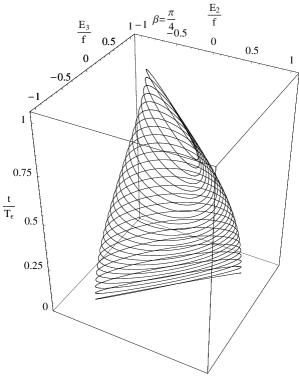
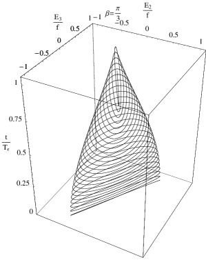
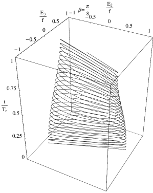
Figure 1: The ellipse described by $E_{2},E_{3}$ is drawn here for three values of $\beta$, along the time axis. We have exaggerated the ratio $\epsilon/\omega$ to $\sim 10^{-2}$, to make the rotation of the polarization plane more evident.

The curve representing (3) is an ellipse with oscillating axes, expressed in terms of $E_{2},E_{3}$, and $f_{2},f_{3}$. For $\epsilon t=0,\pi$, it degenerates in two straight lines $E_{3}=\pm\tan\beta E_{2}$. For $\epsilon=\pi/2,3\pi/2$ we have respectively two ellipses. The ellipse starts with its minor axis being zero and its major axis along the initial plane of polarization. The major axis oscillates and decreases, while the minor axis oscillates increasing, up to a configuration in which the major axis is zero and the minor axis is maximum and passes along the other straight line. Starting from this configuration, the situation is reversed. (See Fig. 1). This effect makes the rotation difficult to be observed in some intervals of time, when one of the semi-axes is very close to zero. We will see below that if some adequate density of electrons exists in the medium, the rotation of the polarization plane is produced at a frequency $\epsilon$ much larger than in the quantum vacuum, allowing it to be observable at magnetic fields and frequencies of the same order as those of PVLAS experiments.

III The case of a medium

The case of photons propagating in a relativistic electron-positron ($e^{\pm}$) medium at temperature $\beta^{-1}\neq 0$ and non-zero particle density (chemical potential $\mu\neq 0$) is of especial interest PerezRojasShabad . The one-loop diagram describing the process accounting for the photon self-energy interaction contains, in addition to the virtual creation and annihilation of the pair, the process of absorption and subsequent emission of one photon by the electron and/or positron. Concerning the average particle densities, for $\mu\neq 0$ but $\beta^{-1}=0$, the average positron density is zero. This is usual in most laboratory conditions.

Also, even in the case of high vacuum conditions of the experiment PVLAS2 , we expect that a density of order $10^{8}$ molecules remain. This is far from being pure quantum vacuum, but a medium which is not invariant under charge conjugation. We assume the existence of a low density electron gas may due to ionization of a fraction of these molecules which might be produced both by the action of the laser beam and the magnetic field intensity. In such case, their equilibrium with ions might be described by some chemical potential $\mu\neq 0$ . The ions also contribute to the self-energy tensor, but due to their large mass, their contribution is much smaller than that of the electron gas. In such a medium, an additional longitudinal electromagnetic wave component is also possible, saturating the three spatial degrees of freedom. Two other tensors, odd in the chemical potential $\mu$ and anti-symmetric in the tensor indices $\rho,\nu$ contribute to $\Pi_{\rho\nu}$ through new basic scalars named $V,R$. The resulting eigenmodes are, in general, polarized elliptically, and in some cases are combinations of transverse and longitudinal waves PerezRojasShabad .

For propagation along the external field $B$ we name $\kappa_{2}=S_{m}$ and $\kappa_{1,3}=T_{m}\pm R$, where $S_{m},T_{m},R$ are scalars depending on temperature and density as well as on $k_{\mu}$ and $B$. The second mode is a pure longitudinal wave, whose electric polarization vector $\textbf{e}^{(2)}=(\omega^{2}-k^{2}_{\parallel})\textbf{b}_{\parallel}\neq 0$ since $k_{\perp}=0$ but $\omega^{2}-k^{2}_{\parallel}$ does not necessarily vanish in the medium. The transverse modes are

$$C^{\prime 1,3}_{\mu}=R(C^{3}_{\mu}\pm iC^{1}_{\mu})$$ (4)

and describe circularly polarized waves in the plane orthogonal to B having different eigenvalues. Up to a normalizing factor, their electric polarization vectors can be written respectively as $\textbf{e}^{(1,3)}=(\textbf{b}^{(1)}_{1}\pm i\textbf{b}^{(3)}_{2})$, corresponding to the eigenvalues $T_{m}\pm R$, leading to the well-known phenomenon of Faraday effect. Let us consider two electromagnetic waves whose polarization vectors are proportional respectively to $\textbf{e}^{(1,3)}$, ($\textbf{h}^{(1,3)}=\textbf{k}\times\textbf{e}^{(1,3)}$).

If we also assume that $T_{m},R\ll\omega$, one can write approximately $\omega_{\mp}=\sqrt{\textbf{k}^{2}-T_{m}}\mp\epsilon^{\prime}$, where $\epsilon^{\prime}=R/2\sqrt{\textbf{k}^{2}-T_{m}}$. Thus, a superposition of both modes having equal amplitudes leads to the following wave

E $$= ARe[\textbf{e}^{1}e^{i(\textbf{k}\cdot\textbf{x}-\omega_{-}t)}+\textbf{e}^{3}e^{i(\textbf{k}\cdot\textbf{x}-\omega_{+}t)}]$$

$$= A[\textbf{e}^{1}e^{-i\epsilon^{\prime}t}+\textbf{e}^{3}e^{i\epsilon^{\prime}t}]Ree^{i(\textbf{k}\cdot\textbf{x}-\omega t)}$$

$$= A(\textbf{b}^{1}\cos\epsilon^{\prime}t+\textbf{b}^{2}\sin\epsilon^{\prime}t)Ree^{i(\textbf{k}\cdot\textbf{x}-\omega t)}]$$

which shows that the polarization of the propagating wave rotates counterclockwise with frequency $\epsilon^{\prime}$, describing a circumference. We recall that as the system has rotational symmetry around B, the direction of the orthogonal eigenvectors $\textbf{b}^{1,3}$ may be taken arbitrarily.

Concerning the propagation perpendicular to the field, we have the eigenvalues $\kappa_{2}=S_{m}$, $\kappa_{1,3}=[(P-T_{m})\pm\sqrt{(P-T_{m})^{2}-4R^{2}}]/2$ which describe two waves whose polarization vector rotates in the plane orthogonal to $B$. However, for very low charge densities, the quantities $P$ and $R$ are negligibly small as compared with $T_{m}$ for perpendicular propagation. This means that the eigenvalues $\kappa_{1,3}$ can be approximated as $\kappa_{3}$, $0$ respectively, the $3$-rd mode being plane polarized orthogonal to $B$. Thus, a wave entering in the magnetized medium propagating orthogonal to $B$, with polarization vector forming some angle $\pi/2>\beta>0$ with B, has components along the polarizations of modes $2,3$. This means that the polarization vector would describe an ellipse with oscillating axes, like the curve mentioned previously in the vacuum case. Below it is shown that its frequency of rotation is approximately a linear function of the electron density, $N_{e}$.

For comparison with PVLAS results, we take frequencies $\omega\sim 1,8\times 10^{15}$ rad/s, and magnetic field $B\sim 5.5\times 10^{4}G$, and we may simplify the expressions given in the Appendix for $T_{m}$ and $F$. Let us call the density of particles by $N_{e}=\sum_{n}(eB/\hbar^{2}c^{2})\int dp_{3}n_{e}$, where $n_{e}$ is the electron Fermi distribution function. We must stress here that $n_{e}$ stands for the low temperature limit of the sum of electrons plus positrons densities $n_{e}+n_{p}$, ($n_{p}$ is negligible small at low temperatures), since the Cotton-Mouton rotation exists in any case, even in a neutral electron-positron gas, where $n_{e}=n_{p}$ as different from the Faraday rotation, which depends on the net charge $n_{e}-n_{p}$. We may approximate $(\ref{T})$ and $(\ref{S})$ given in the Appendix as

$$T_{m} = -\frac{2\alpha}{\pi}\lambda^{3}m^{2}c^{4}N_{e}$$ (6)

$$S_{m} = -\frac{\alpha}{\pi}\lambda^{3}m^{2}c^{4}N_{e},$$ (7)

since $(\ref{T})$ and $(\ref{S})$ under the conditions of propagation perpendicular to $B$, $k_{\perp}^{2}\ll m^{2}c^{4}$ and near the light cone ($k_{\perp}\sim\omega$) are approximately independent of the photon momentum and energy. Here $\lambda$ is the electron Compton wavelength. The dependence on $B$ is contained in the term $N_{e}$ (see below). We assume that to have charge neutrality one must add to (6, 7) a similar term in which the electron density is replaced by the ion density and the electron mass by the ion mass. Such term, however, is al least $10^{-3}$ times smaller than expressions (6),(7), and may be ignored in the calculations.

For the previous values of $B$ and $\omega$, we have finally $\Delta\omega=(S_{m}-T_{m})/k_{\perp}\sim\frac{\alpha}{\pi}\lambda^{3}m^{2}c^{4}N_{e}/k_{\perp}\sim 5,6\times 10^{-34}N_{e}$. For $N_{e}\sim 10^{3}$, $\epsilon\sim 10^{-31}erg=10^{-4}$ rad/s, leading to a period $T\sim 10^{4}$ s. The angle rotated in a length of one meter is of order $10^{-13}$ rad.

Eqs. (6),(7) are valid for any value of the electron density and energy. Their dependence on the magnetic field is contained in the density of particles term: for constant chemical potential and zero temperature, the dependence on $B$ comes from the degeneracy factor $eB$ and from the energy eigenvalues $E_{n}$, especially for nonzero temperature. However, another dependence might come from the chemical potential $\mu$, which may be $B$-dependent.

Thus, for having a Cotton-Mouton rotation comparable with the limits imposed by the last results of PVLAS experiments PVLASII , if on the average, and in the process of the experiment, the system behaves as if having a number of free electrons of order $0.001$ percent of the remnant molecules. This is enough to give a figure $10^{3}$ times the pure quantum vacuum effect.

The Fermi-Dirac degenerate distribution might not be suitable to describe $n_{e}$ in some cases, for instance, at nonzero temperature and very low densities. Thus, although the experimental PVLAS conditions are made at temperatures near zero, the observed phenomenon occurs far from equilibrium. For a fixed magnetic field we may assume that on the average it behaves equivalently to an equilibrium system having a constant chemical potential and an effective temperature of several Kelvin degrees, and use the Boltzmann distribution $n_{e}=\sum\alpha_{n}\int dp_{3}e^{-((E-\mu))\beta}$ ($\alpha_{n}=2-\delta_{0n}$), as an approximation. For $E$ we take the non-relativistic limit by expanding it as $E=mc^{2}+p^{2}/2m+eB\hbar n/mc$. We call $A=e^{-\mu^{\prime}\beta}$, where $\mu^{\prime}=mc^{2}-\mu$, and gets easily

$$N_{e}=A\frac{eB}{\lambda_{D}\hbar c}\coth\frac{eB\hbar\beta}{mc}$$ (8)

where $\lambda_{D}=\hbar/\sqrt{2\pi m/\beta}$ is the De Broglie thermal wavelength. For for $\mu^{\prime}$ constant and $X<1$, by taking $cothX\sim(1/X+X/3)$, we conclude that $N_{e}$, and in consequence $\epsilon$ grows with $B$ as $a+bB^{2}$, where $a=m/\lambda_{D}\hbar^{2}$,$b=e\hbar\beta/mc$ are temperature dependent parameters. For $T$ of order of few Kelvin degrees, the dominant term is $a$ which is independent of $B$. But the chemical potential might be dependent on $B$, which is more realistic for the ionization process. Thus, for the dilute gas under the influences of both the laser and magnetic field it is expected for $T_{m}$, $S_{m}$ a dependence on $B$ more complex than in the quantum vacuum case (i.e. not proportional to $B^{2}$)

We must observe that formulae (10,12) in the Appendix may be applied even in the case of the so-called hot vacuum, a system of electron-positron pairs in equilibrium with photons at high very high temperature ($\beta^{-1}\geq mc^{2}\sim 10^{9}$ ^∘K), Such a system have zero net charge, and is invariant under charge conjugation. Such system (which might exist in neutron stars magnetospheres) does not exhibit the Faraday rotation but it shows the Cotton-Mouton rotation of the polarization plane. Even more, as hot vacuum implies $\mu=0$, and the Boltzmann distribution is a good approximation for it Kratkie one can use the expressions below (6,7) and (8) by taking $A=2e^{-\beta mc^{2}}$. It is seen from (8) that by increasing temperature, the density of particles, and in consequence, the frequency induced by the magnetic field, decreases.

In concluding, we want to emphasize that the Cotton-Mouton rotation of the polarization plane for photons propagating orthogonal to $B$, although bears some analogy to Faraday effect, differs from it in two main facts: Faraday rotation is circular (which is related to the axial symmetry determined by the preferred direction of magnetic field $B$, whereas the Cotton Mouton rotation is a more complex curve; Faraday rotation occurs only if the system is not invariant under charge conjugation, whereas Cotton-Mouton rotation does not require non-invariance under charge conjugation. Thus, it occurs in QED vacuum, in a medium containing an electron-ion system, as well as in a neutral molecular or electron-positron gas. Even if the remnant ionized molecules density would be negligible small, the medium would show birefringence properties, with the consequent rotation of the polarization plane. The Cotton-Mouton rotation is expected to act on the polarization plane of radiation propagating across intergalactic media.

The authors thank the Abdus Salam ICTP support under OEA-ICTP Net-35 Grant. They thank M. Chaichian, A. Tureanu and A. Zepeda for several comments and discussions, to A. Gonzalez, B.Rodriguez and S. Villalba for valuable suggestions, and especially to A.E. Shabad for several important remarks.

IV Appendix:

a)We write the explicit expressions for $S$ and $T$ in quantum field theory ShabadAP , in which it is taken $\hbar=c=1$, and in statistics PerezRojasShabad . In the first case,by calling $z_{2}\equiv k_{\perp}^{2}$, the scalars $\kappa_{2,3}=S,T$ are given by

$$\kappa_{2,3}=\frac{2\alpha}{\pi}\int_{0}^{\infty}d\tau\int_{1}^{1}d\eta[\rho_{2,3}C]e^{M-\frac{N}{2\tau}}e^{-\tau m^{2}}$$ (9)

where

$$C=\frac{eB}{\sinh eB},N=\frac{1-\eta^{2}}{4},M=-\frac{1}{2}z_{2}M^{\prime}-\frac{1}{2}z_{1}N$$

$$\eta^{\pm}=\frac{1\pm\eta}{2},M^{\prime}=\frac{\sinh eB\tau\eta^{+}\sinh eB\tau\eta^{-}}{eB\sinh eB\tau}$$

$$\rho_{2}=-\frac{1}{2}z_{1}\cosh eB\tau N-\frac{1}{2}z_{2}Q$$

$$\rho_{3}=-\frac{1}{2}z_{2}CM^{\prime}-\frac{1}{2}z_{1}Q$$

$$Q=\eta^{-}\frac{\sinh eB\tau\eta^{+}\cosh eB\tau\eta^{+}}{\sinh eB\tau}$$

One can expand (9) in powers of $z_{1}$, $z_{2}$. To first order one gets

$$\kappa_{2,3}(z_{1},z_{2})=z_{1}(\frac{\partial\kappa_{2,3}}{\partial z_{1}})_{z_{1}=z_{2}=0}+z_{2}(\frac{\partial\kappa_{2,3}}{\partial z_{2}})_{z_{1}=z_{2}=0},$$

since $\kappa_{2,3}(0,0)=0$. By taking the expansion in powers of $B^{2}$ also to first order, one gets eqs. (1), (2).

b) We shall now write from PerezRojasShabad ,PerezRojas the explicit expressions for the scalars $R$, $T_{m}$ and $S_{m}$ for $\omega^{2}\hbar^{2}\ll 2eB\hbar c$, in the case of a charged medium, i.e. , in relativistic quantum statistics. We have

$$T_{m}=-\frac{eB\hbar c}{4\pi^{2}}\sum_{n,n^{\prime}}F^{(2)}_{n,n^{\prime}}\int_{-\infty}^{\infty}\frac{dp_{3}}{E_{q}}[1-G](n_{e}+n_{p}-1)$$ (10)

where $G=[(H+N)K]/|Q|^{2}$, where $H=z_{1}+2eB\hbar c(n+n^{\prime}))$, $K=z_{1}+2eB\hbar c(n^{\prime}-n)$, $|Q|^{2}=K^{2}-4\omega^{2}E_{q}^{2}$, and $n_{e}$,$n_{p}$ are the electron and positron Fermi-Dirac distribution functions. The quantity $-1$ subtracted to them stands for the quantum field limit $\mu\to 0$, $\beta^{-1}=0$, whose contribution to order $B^{2}$ was discussed previously. The quantity $E_{q}=\sqrt{m^{2}c^{4}+c^{2}p_{3}^{2}+2eB\hbar cn}$ is the electron-positron energy eigenvalue. The quantities $F^{(2)}_{n,n^{\prime}}$, $N=4N^{(1)}_{n,n^{\prime}}$ are defined in PerezRojasShabad , as well as $F^{(1,3)}_{n,n^{\prime}}$ and $G^{(1)}_{n,n^{\prime}}$, used below, in terms of the Laguerre functions of the variable $k_{\perp}^{2}/2eB$. They have the property $F^{(2,3)}_{n,n^{\prime}}(0)=\delta_{n,n^{\prime}-1}\pm\delta_{n-1,n}$, $F^{(1)}_{n,n^{\prime}}(0)=\delta_{n-1,n^{\prime}-1}+\delta_{n,n^{\prime}}$, $G^{(1)}_{n,n^{\prime}}(0)=2(\delta_{nn^{\prime}}+\delta_{0n})$,$N^{(1)}_{n,n^{\prime}}(0)=0$ PerezRojas .

Now we give the corresponding expression for $R$. We have $R=\sqrt{\frac{k^{2}}{z_{1}}}F$, where

$$F=-\frac{eB\hbar c}{4\pi^{2}}\sum_{n,n^{\prime}}F^{(3)}_{n,n^{\prime}}\int_{-\infty}^{\infty}\frac{dp_{3}}{E_{q}}[H](n_{e}-n_{p}).$$ (11)

The term $F$ arises due to the electron-positron charge asymmetry. It vanishes in the limit $\mu\to 0$, but is nonzero in absence of positrons, whenever the electron density $n_{e}\neq 0$.

The expression for $S_{m}$, which in the present case contributes to the expansion to first order in $\omega^{2}$.

$$S_{m} = -\frac{eB\hbar c}{2\pi^{2}}\sum_{n,n^{\prime}}\int_{-\infty}^{\infty}\frac{dp_{3}}{E_{q}}[L]\frac{K}{|Q|^{2}}(n_{e}+n_{p}-1)$$ (12)

where $L=2m^{2}c^{4}+eB\hbar c(n+n^{\prime}))F^{(1)}_{n,n^{\prime}}+eB(nn^{\prime})^{1/2}G^{(1)}_{nn^{\prime}}$. For $\beta^{-1}\to 0$, (i.e., for all practical purposes in most laboratories) the positron contribution vanishes in (10,12), and we omit it in what follows). For propagation parallel to $B$, $k_{\perp}=0$ and the argument $F^{(1,2)}_{n,n^{\prime}}$ vanish. In the approximation assumed above ($\omega^{2}\hbar^{2}\ll 2eB\hbar c$)these expressions are actually valid also for propagation perpendicular to B. This makes $\int(n_{e}dp_{3})/E_{q}$ the dominant term in the integrals in $T_{m},S_{m}$.

c)We return to the Faraday rotation problem. We have

$$F=-\frac{\alpha}{2\pi}\frac{mc^{2}\lambda^{3}eB\hbar cN_{e}}{\hbar\omega}$$ (13)

For propagation parallel to $B$ we have,

$$T_{m}\sim 10^{-45}N_{e},\\ R=F\sim 10^{-48}N_{e}$$

By dividing $R$ by the factor $|\textbf{k}|\sim 10^{-12}$ erg we get

$$\Delta\omega=R/k\sim 10^{-36}N_{e}$$

Thus, $\epsilon^{\prime}/\omega=\Delta\omega/\omega\sim 10^{-24}N_{e}$. A density of $10^{6}$ electrons/cm³, would give a Faraday rotation frequency whose order of magnitude is comparable with PVLAS rotation.

.

References

- (1) A. E. Shabad, Ann. Phys. 90, 166-195 (1975)
- (2) H. Perez Rojas, A. E. Shabad, Ann. Phys. 121, 432-455 (1979)
- (3) E. Zavattini et al., Nucl. Phys. Proc. Suppl.164, 264-269 (2007)
- (4) I. A. Batalin, A. E. Shabad, J. Exp. Theor. Phys. 60, 894-900 (1971)
- (5) W. Heisenberg and H. Euler, Z. Physics , 98, 714 (1936)
- (6) J. Schwinger, Phys. Rev. 82, 664 (1951)
- (7) S. L. Adler, Ann. Phys. 67, 559 (1971)
- (8) A. E. Shabad, J. Exp. Theor. Phys. 98, 186-196 (2004)
- (9) H. Perez Rojas, J. Exp. Theor. Phys. 76,1,(1979)
- (10) W. Dittrich and H. Gies, Phys.Rev.D58, 025004,(1998).
- (11) Ugo Gastaldi,arXiv:hep-ex/0507061
- (12) H. Perez Rojas and A.E. Shabad, Kratkie Soobcheniya po Fizike (Lebedev Institute Reports, Allerton Press), 7 (1976) 16.
- (13) E. Zavattini et al, arXiv:hep-ex/0706.3419v3