3D Spectroscopy and the Virtual Observatory

Abstract

Integral field, or 3D, spectroscopy is the technique of obtaining spectral information over a two-dimensional, hopefully contiguous, field of view. While there is some form of astronomical 3D spectroscopy at all wavelengths, there has been a rapid increase in interest in optical and near-infrared 3D spectroscopy. This has resulted in the deployment of a large variety of integral-field spectrographs on most of the large optical/infrared telescopes. The amount of IFU data available in observatory archives is large and growing rapidly. The complications of treating IFU data as both imaging and spectroscopy make it a special challenge for the virtual observatory. This article describes the various techniques of optical and near-infrared spectroscopy and some of the general needs and issues related to the handling of 3D data by the virtual observatory.

1 Introduction

A basic goal of observational astronomy is to obtain the most complete, unbiased description of the objects under study. A complete description of an astronomical observation is inherently multi-dimensional, at each position on the sky one can measure intensity, wavelength or energy, and up to four polarization (Stokes) parameters. Each of these quantities can also vary with time. Since almost all astronomical objects have properties that are complex — structures on all scales, asymmetries, gradients, and variability — there is a strong need to obtain full 2D (spatial) information of all observables. The maximizes the information content of the observations and provides the most constraints possible for comparison with models and theories.

However, the nature of light and the technological limitations of instruments and detectors in general prevent us from making the “perfect” observation. Radio and sub-mm interferometric observations come the closest to the ideal. A map of the UV plane provides intensity, frequency (energy), and polarization information. The data cube does contain time information as well, though usually repeated observations are often needed to study variability. Many modern 2D X-ray detectors are also inherently multi-dimensional since the time and energy of each photon are recorded. However, obtaining high energy resolution usually means the loss of one spatial dimension.

Likewise, in the optical and near-infrared (NIR) the available technology limits the number of dimensions that can be observed simultaneously. Sensitive photon-counting systems such as photo-multiplier tubes, avalanche photo-diodes, and superconducting tunnel-junction devices (de Bruijne et al., 2002) are ideal for studying intensity variability on short timescales, but they have low energy resolution and are either single-channel devices or small arrays and so are inefficient for studying large areas of sky or for doing high-resolution spectroscopy. All large-format detectors such as photographic plates and CCDs are two dimensional and while they are good at counting the number of photons they have poor intrinsic energy resolution. Therefore, optics must be used to separate different wavelengths. Simply placing a dispersive element in the light path is one valid solution. While this “slitless” spectroscopy can be a useful way of obtaining spectral information over a full 2D field, it has the disadvantages of high background noise in ground-based observations, spectral resolution dependent on image quality, and confusion in crowded regions. Slitless spectroscopy has been used extensively to search for emission lines in limited wavelength regions (e.g. Salzer et al., 2000; Douglas et al., 2002). The background and spectral resolution problems are often solved by isolating the region of interest with a slit; spectra are obtained only along one physical dimension and the second dimension of the detector contains the wavelength information. This is very appropriate for compact isolated objects, but mapping large areas of extended, complicated sources with a slit is time consuming and it can be difficult to register spatially dithered spectra. Also, obtaining spatially contiguous spectra is usually not possible.

However, in the last 30 years clever optical/NIR instrument designers have developed 3D ($x,y,\lambda$) techniques that produce spectra of moderate to high resolutions ($R>100$) over a contiguous field. Other advantages of these techniques are easier acquisitions (no need to center precisely in a slit), radial velocities that are not affected by slit-centering errors, and no light losses that are otherwise unavoidable with narrow slits. These techniques were considered rather specialized at first but in the last 10 years the advantages of the techniques and the successes of the early 3D, or integral-field, spectrographs have made them popular and very common. Most current and future large optical/NIR telescopes have or will have integral-field options in their standard instrument suites.

Therefore, IFU (integral-field unit) data is becoming more and more common in telescope archives Also, large surveys such as SAURON and Atlas3D (de Zeeuw et al., 2002; Krajnović, 2007) are being carried out now and even more ambitious projects are being planned (see below). Thus, it is important for the Virtual Observatory (VO) to support integral-field data. This is a challenge because it requires a combination of imaging and spectroscopic techniques. However, since IFU data is still relatively new and many common reduction packages do not include good tools for manipulating IFU data, there is an opportunity for the VO to set standards and create useful tools that will draw people to the VO.

The remainder of this proceedings will review the different types of optical/IR spectrographs and the different formats of data that are being produced. Then some basic requirements for handling and visualizing IFU data in the VO will be discussed.

2 Optical/IR 3D Techniques

The two main types of optical/IR 3D instruments are spectrometers and spectrographs. Within each type there are a variety of related designs. This section will review the basic features of the most common variations. Some other good recent technical reviews of different 3D techniques are Bennett (2000) and Allington-Smith (2006).

2.1 Spectrometers

The fundamental principle of a spectrometer is that the wavelength region of interest is scanned in discreet steps and a narrow-band 2D image is taken at each wavelength, thus building up a stack of 2D images, or cube. Interference techniques are used to make the adjustable narrow-band filters.

One of the most common types of 3D spectrometer is the imaging Fabry-Perot, sometimes called a tunable filter, in which the interference between two closely spaced and adjustable partially-transmissive plates creates a narrow bandpass. There are also a variety of related techniques (Bland-Hawthorn, 2000). The main advantage of the tunable filter is that it can have a very wide field, up to several arcminutes in diameter. However, the spectral resolution is relatively low, between 100 and 1000, and often $R$ and wavelength coverage must be traded off against each other. Examples of this type of instrument are the Taurus tunable filter that has been used on the AAT and WHT and GRIF behind the adaptive optics system at the CFHT (Clénet et al., 2002). Also, several new tunable filters are being commissioned or developed, including the Maryland-Magellan Tunable filter (Dressler et al., 2006), FTF2 for the Flamingos 2 NIR MOS spectrograph for Gemini South (Scott et al., 2006), and the OSIRIS instrument on the GTC (Castañeda et al., 2002).

One other 3D spectrometer is the Imaging Fourier Transform Spectrometer (FTS) in which a FTS a Michelson interferometer defines the bandpass. These instruments have smaller fields-of-view, typically less than 1 arcminute, but the spectral resolution can be as high as about 30000. The FTS is sensitive to shot noise from the sky so ground-based observations will often use a bandpass filter to limit the spectral range. Figure 1 shows an example image from the Bear FTS spectrometer on the CFHT (Cox et al., 2002)

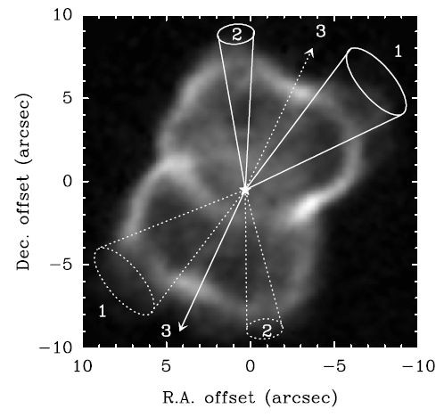
Figure 1: A 3D spectrometer result from the imaging FTS BEAR on the CFT (Cox et al., 2002). This shows the velocity-integrated H₂ emission from the planetary nebula NGC 7027. Outflow axes identified from the data cube are labeled.

The data format of a 3D spectrometer is a regularly gridded 3D ($x,y,\lambda$) datacube. Each ($x,y$) plane is a typical image which can be manipulated by most image processing software. This data is similar to a radio datacube and is the easiest to process and visualize with current software.

The main drawbacks of spectrometers are that the spectral range is relatively small and, more importantly, that the spectra are not created simultaneously. Therefore, any changes in image quality, sky transparency, and background during the scan will make the spectra difficult to process and interpret.

2.2 Spectrographs

Integral field spectrographs (IFSs) are a more spectra-based approach to 3D spectroscopy than the spectrometers. There are three basic flavors of IFS concepts — lenslet only, fiber based, and image slicer — each with particular advantages and applications (Figure 2). In all the flavors optics are used to sample the focal plane into “spaxels” (spatial pixels) and then the light from each is dispersed by a standard grating or grism spectrograph. Therefore, the spectral resolution is dependent on the ruling of the grating/grism and the effective size of the entrance aperture. Most IFSs operate with spectral resolutions between 500 and 5000. An advantage of the IFS is that all of the spectra are obtained simultaneously. However, since detector area is needed to store all the spectra the field-of-view (FOV) has to be sacrificed. The largest fields are about an arcminute in diameter. Techniques of modifying the field size include using fore-optics to change the scale (arcsec/mm), trading off FOV for spectral coverage, and by increasing the detector area by using bigger CCDs or CCD mosaics. Some dedicated IFSs exist but often a multi-purpose spectrograph can be given 3D capability by inserting an integral-field unit (IFU) into the focal plane as if it were a standard slit mask.

The first and simplest IFSs were derivatives of the early fiber multi-object spectrographs (MOS). In this design the input ends of the optical fibers are packed as closely together as possible in the focal plan and then the fibers reformat the 2D field into a pseudo slit at the entrance to the spectrograph (Vanderriest, 1980). Since these IFUs are relatively easy to construct and incorporate with existing spectrographs quite a few have seen operation, including SILFID at CFHT (Vanderriest & Lemonnier, 1988), INTEGRAL at the WHT (Arribas et al., 1998), and DensPak and SparsPak at WIYN (Barden & Wade, 1988; Bershady et al., 2004). The disadvantages of this design are that the spatial coverage is not contiguous because of the cladding needed to support the fibers and that throughput losses occur due to focal ratio degradation (FRD) caused by feeding the fibers with a slow telescope beam (see Allington-Smith et al., 2002).

The problems of the fiber-only IFU can be avoided by using a microlense array to sample the focal plane (Courtes, 1982). The microlenses give full, contiguous spatial coverage and focus an image of the telescope pupil on the spectrograph entrance. In lenslet-only IFSs (Figure 2) the spectrograph input is an array of micropupil images. If grisms are used to disperse the light then the optical design can be quite simple and have high throughput. However, a blocking filter must be used to limit the spectral coverage in order to avoid spectral overlap in the dispersion direction. Thus, the spectral coverage is always limited. Also, in the cross-dispersion direction neighboring spectra overlap at different wavelengths. The spectra cannot be positioned too closely together and deconvolution is mandatory to extract the spectra (Bacon et al., 2001). Field of view is made adjustable by fore-optics that change the scale (arcsec/mm) at the lenslet array. Examples of productive lenslet-only IFSs are TIGRE on the CFHT (Bacon et al., 1995), OASIS and SAURON on the WHT (Bacon et al., 2001), and OSIRIS on Keck (Larkin et al., 2006). Figure 3 shows a classic IFS result, the kinematically decoupled central disk in a velocity map from SAURON (Davies et al., 2001).

Lenslet arrays are also used to focus pupil images onto the entrances of fibers. Lenslet-fiber IFUs have full spatial coverage and avoid the FRD losses of fiber-only designs. Another advantage is that the spectra can be more tightly packed on the detector since neighboring spectra on are adjacent on the sky and in wavelength (Allington-Smith et al., 2002). This makes more efficient use of detector area and helps produce larger fields-of-view. Deconvolution of overlapping spectra is still helpful, but not mandatory. With IFUs of this type is often possible to trade field-of-view for spectral coverage. For example, in the Gemini GMOS IFUs (Allington-Smith et al., 2002) and the ESO VIMOS IFU (Bonneville et al., 2003) the full field is divided into equal sections. Fibers transfer the light from each section to pseudo slits at the spectrograph(s) entrance(s). When the largest field-of-view is required blocking filters must be used to limit spectral coverage and avoid overlap. When higher spectral resolution or longer wavelength coverage is desired then some of the pseudo slits can be masked off to increase spectral coverage at the expense of FOV. This type of IFU has become very popular. In addition to the GMOS-N/S and VIMOS IFUs mentioned above, other examples include CIRPASS on Gemini, the AAT, and the WHT (Parry et al., 2004), PMAS on Calar Alto (Roth et al., 2005), SPIRAL at the AAT (Sharp et al., 2006), MPFS on the SAO 6-m, IMACS on Magellan (Schmoll et al., 2004), and FLAMES on the VLT (Pasquini et al., 2002).

The final common type of IFS is the image slicer. In this design the focal plane of the telescope is sampled by a stack of diamond-turned slicing mirrors. An optics train then reformats the 2D field ($x,y$) into a 1D pseudo slit at the spectrograph entrance. The 2D spectra ($x,\lambda$) from the slices are lined up side-by-side on the detector. Slicer IFU units can be very compact and the all-reflecting optics make them good for cryogenic environments. Therefore, they are often used for near and mid-IR IFUs. Slicer IFUs currently in use include 3D from MPE (Weitzel et al., 1996), PIFS at Palomar (Murphy et al., 2000), UIST at UKIRT (Ramsay Howat et al., 2006), ESI at Keck (Sheinis, 2006), GNIRS and NIFS at Gemini (Allington-Smith et al., 2006; Hart et al., 2003; Miller et al., 2006), and SPIFFI at the VLT (Iserlohe et al., 2004).

The native data format for each of these instruments tends to be unique. For fiber and lenslet IFSs the reduced dataset is a set of 1D spectra, one for each lenslet/fiber spaxel, and a table of the relative positions of each spaxel on the sky. Often the lenslets are hexagonal so this type of data does not naturally produce a rectangularly gridded 3D cube. The slicer IFUs produce a set of ”longslit” spectra that are easier to place into a regular cube.

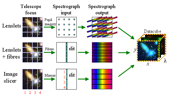
Figure 2: A schematic of the three main types of integral field spectrographs: lenslet-only, lenslet$+$fiber (or fiber only), and image slicer. The three techniques can produce very similar 3D data but the information density on the detector increases from top to bottom (lenslet only to image slicer). (Figure credit: Jeremy Allington-Smith)

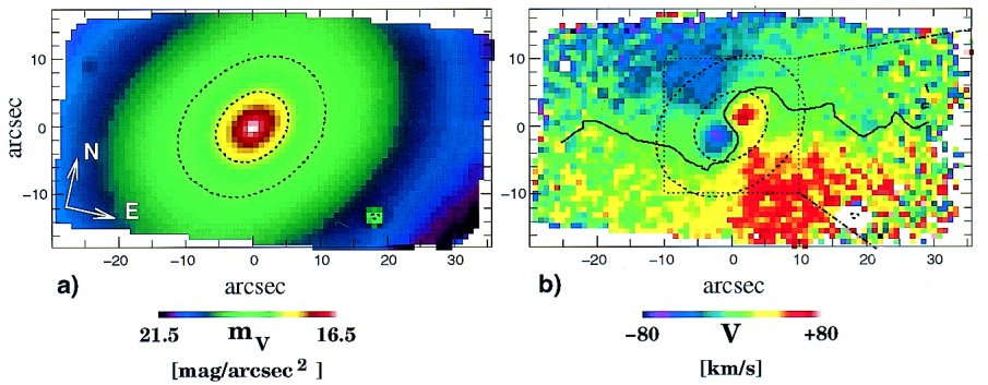
Figure 3: The integrated light (a) and velocity field (b) of the inner region of the elliptical galaxy NGC 4365 (Davies et al., 2001). The galaxy has a small inner disk rotating around the minor axis but stars in the outer galaxy are rotating around the major axis.

2.3 IFU Surveys

IFSs are increasingly being used for large surveys. The SAURON instrument on the WHT was conceived as a survey instrument and the initial survey of about 70 galaxies has already revealed important new insight into the dynamics and formation of elliptical galaxies (Emsellem et al., 2007; Cappellari et al., 2007). Atlas3D is an extension of the SAURON survey that will observe nearly 200 early-type elliptical galaxies to produce a complete sample of early-type galaxies brighter than $M_{K}=-21.8$ within 40 Mpc (Krajnović, 2007). New IFSs for surveys are now under development. VIRUS on the HET is a massively-modular IFS being constructed for the HETDEX galaxy redshift and dark energy experiment (Hill et al., 2004). KMOS is a NIR IFS being built for the VLT which will have 24 slicer units with pickoff mirrors on deployable arms (Sharples et al., 2006). It will compile statistics on the kinematics of distant galaxies similar to what SAURON has done for nearby galaxies. Another new IFS for the VLT is MUSE (Bacon et al., 2004). It will have 24 spectrograph modules making up a 1 arcminute field. It is designed to work behind a ground-layer adaptive optics system that should routinely produce $0.3-0.4$ arcsec image quality. It will be a general-purpose IFU studying deep fields of distant galaxies, nearby galaxy kinematics, and solar system objects.

2.4 IFUs with Adaptive Optics

If the 1990s was the era when the 8-10 meter became the norm, the 2000s is the time of the common use of adaptive optics (AO) and laser guide stars (LGS). Such systems are in use or currently under development at Keck, Gemini, ESO and the GTC they will probably be an integral part of the next generation of giant telescopes (Crampton & Simard, 2006; Cunningham et al., 2006). These systems produce near-diffraction-limited images that rival or surpass the images from smaller space telescopes. To take advantage of the image quality spectrographs with AO should have correspondingly narrow slits. However, normal variations in image quality and the “breathing”, or plate scale changes normal to single-star AO systems could lead to significant slit losses with a normal slit spectrograph IFSs overcome these problems since slit losses are not an issue. IFSs used with AO systems have small fields, normally around 3 arcseconds, because of the fine sampling needed, but they provide spectroscopy while preserving the high image quality. IFSs being using with AO systems now include OASIS at the WHT, GRIF at CFHT, NIFS at Gemini North, SINFONI at the VLT, and OSIRIS at Keck. An IFU will also be used with the high-contrast AO system of the Gemini Planet Imager (Macintosh et al., 2006).

2.5 IFUs on JWST

IFUs will also be major components of the instrumentation for the 6.5-meter James Webb Space Telescope (JWST) being constructed by NASA, ESA, and the CSA. JWST will include three 3D spectroscopy technologies. A Fabry-Perot tunable filter to be provided by the CSA with a 2.2 arcminute field of view will be part of the fine guidance sensor (Rowlands et al., 2004). It will provide narrow-band imaging with $R~{}100$ and will also have a chonographic mode. Also, the ESA NIRSpec spectrograph will contain a slicer IFU with a 3 arcsecond field-of-view and 0.1 arcsec slices (Arribas et al., 2005). Finally, the medium resolution spectrometer in the mid-infrared instrument MIRI is a slicer IFS with four slicers in separate wavelength channels split by dichroics (Wright et al., 2004).

3 3D Spectroscopy and the Virtual Observatory

The increasing popularity of optical/IR 3D data and the large volume of 3D data that will soon be in archives makes it very important that 3D spectroscopy is supported by the VO. As with any form of astronomical data, the main issues that have to be addressed are data description, storage format, discovery, data transmission, and analysis tools. 3D data provides an interesting challenge because it is a mixture of imaging and spectroscopy. Fortunately, this means that existing protocols and tools for handling imaging and spectroscopic data separately can serve as a basis for handling 3D data. A goal is that an astronomer could be able to use the VO to find and combine multi-wavelength 3D data on an object (a 3D SED) and then do analysis on this meta-cube. With the addition of multiple observations to give the time information, we are approaching the goal of the fully general observation.

3.1 Data Description

A meta-data structure, or general data model, for describing optical/IR 3D data has been developed using the IVOA Simple Spectra Access Protocol (Chilingarian et al., 2006). More details about this standard and an example application are given in (Chilingarian et al., 2007).

3.2 Storage Format

The storage format for 3D data is an important consideration for discovery, transmission, and analysis. As has been mentioned, each IFU tends to have its own data format. This is partially due to the fact that the most commonly used data reduction packages such as IRAF, MIDAS, and IDL, do not have a common data structure for 3D data. Also, there is the problem that different types of instruments produce different types of data: stacks of images; one spectrum per spaxel; or a series of 2D “longslit” spectra. A common data format for reduced data would help promote the use IFU use by making it easier to develop analysis tools. A common format would also simplify making IFU data VO compliant.

One option for a standard IFU data format is the Euro3D format developed by the European OPTICON Euro3D research training network (Kissler-Patig et al., 2004). The format is a 3D FITS table in which each row contains the information from one spaxel. Columns can contain coordinate information and data, data quality, and statistics vectors. It is general to all IFS instruments after the instrument signature is removed. It also has a very general spatial description of a spaxel that does not require resampling to a 3D linear cube and that supports adaptive binning (Cappellari & Copin, 2003).

Another option for a common format is the linearly sampled 3D FITS cube. This gives the data a similar format to radio and 3D spectrometer data cubes and it makes the data a bit easier to visualize with common display tools. However, it would require that many IFS datasets be re-sampled (which can often degrade data) and it doesn’t lend itself to adaptive binning. Data that is not on a regular grid should not be forced into one unnecessarily. However, because of the meta-data description it should be possible to support both Euro3D and datacube formats.

3.3 Discovery

Data discovery needs to answer the user questions “What data is available?” and “Is it useful to me?”. If the answer to the second question is “yes” then the astronomer will continue to work on the data by downloading it or analyzing it with VO tools. For 3D data good query interfaces must be joined with both imaging and spectral visualization tools. Searches need to be done both in terms of position and wavelength. It should be possible to visualize the footprint of IFU data on a digital sky image. Then it should be possible to preview both image and spectral representations of the 3D dataset. A first-generation tool that fulfills many of these requirements is described by Chilingarian et al. (2007) in this volume.

3.4 Data Transmission

Full Euro3D or datacube files can be many megabytes in size and new instruments like VIRUS and MUSE will produce vastly larger datasets than current instruments. Therefore, it is important that it be possible to extract regions of a dataset. Because of the size and complexity of 3D data, data providers should experiment with providing processing and analysis on the server. However, the users should always have the option to download the data for local analysis.

3.5 Visualization and Analysis Tools

As has been mentioned several times, visualization and analysis of 3D data is challenging because of the combination of needs for manipulating images and spectra. It is always important to be able to treat a 3D dataset as a set of images. It is often useful to loop through the planes like a movie. For IFS data this means that the tool needs to reconstruct the images and show any binning that was done. Registering and either overlaying or overplotting different planes or different images are also needed. Also, it should be possible to select a wavelength range and inspect the resulting 2D spatial map. Inversely, one should be able to select a region from a map and then inspect either the individual spectra or the summed or averaged spectrum. As with imaging, overplotting is an important feature. Two 3D visualization tools that do many of these things are the Euro3D tool (Sánchez, 2004) and QFitsView (Abuter et al., 2006). However, neither is VO compliant at this time. Another potentially powerful visualization option is to treat the spatial and spectral dimensions together. A few visualization labs and authors have been experimenting with generating 3D views of IFU data by using volume rendering, stereoscopic views or “3D” display monitors, and holographic imaging (see Figure 4). These techniques make full use of the data and can help astronomers draw the correct physical interpretation. Generating good visualization tools for 3D data is a challenge but also an important opportunity for the VO community.

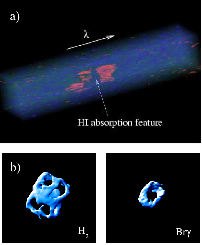
Figure 4: Volume renderings of 3D data cubes. a) Ly$\alpha$ emission and absorption from a $z=3.09$ galaxy observed by SAURON (Wilman et al., 2005). b) Representations of the H₂ and Br$\gamma$ emission from the planetary nebula NGC 7027 (Cox et al., 2002). The outflow cavities sketched in Figure 1 are clearly seen.

Until now we have been treating the spectral and spatial domains independently, however, certain operations on 3D data require that they be treated simultaneously. One example is the need to subtract a spectral continuum from a region using an annulus around it. This would involve fitting in both wavelength and position. Also, both spatial and spectral PSFs change with wavelength so a deconvolution of either quantity involves deconvolution in both. For example, atmospheric refraction is a shift of spatial position with wavelength and correcting for it requires operations in all dimensions of the dataset (Arribas et al., 1999). Finally, adaptive binning is a means of combining adjacent spaxels until the spectral signal-to-noise is sufficient for a particular analysis. All these operations mean that the errors in the spectra of adjacent spaxels become correlated so error propagation is very important for the final assessment of signal-to-noise.

The analysis needs in only the spectral dimension are fairly standard, only it must be easy to apply the same analysis to all spaxels in a dataset. The main needs are single and multiple line fitting, radial velocity and velocity dispersion measurements using observed templates or models, and the measurement of line fluxes, equivalent widths, and line indices. Radial velocity measurements and stellar template fitting to separate the emission line and absorption line spectra are good applications for the VO since the template observations or models could be accessed via the VO. This also meshes with the VO focus on SED fitting which should be generalized to 3D.

Once a 2D map is produced it should be possible to perform all standard imaging analysis on it. This includes calculating statistics, aperture photometry, ellipse or isophote fitting, fitting surfaces, and the subtraction of background regions. In addition, many maps may not represent intensity data but the results of the spectral analysis such as velocity fields or line ratio maps. These maps may also need quantitative analysis. An example of this is kinemetry, a Fourier analysis of line-of-sight velocity distributions similar to ellipse isophote fitting that provides a quantitative description of velocity fields (Krajnović et al., 2006).

More advanced capabilities can also be envisioned. For example, it is likely that an investigator would want to apply new and perhaps proprietary techniques or models to data available with the VO. For example, someone could want to fit N-body models to velocity fields from a 3D instrument. This person could download the data to fit to the models, but if the dataset is very large it may be more efficient to upload the model or analysis technique to the data on the server and let the powerful server handle the processing. In cases like this the intellectual property of the user would have to be respected and the use of expensive processing resources might need to be negotiated.

4 Summary

Three dimensional spectroscopy techniques in the optical and NIR are a relatively new but rapidly growing in importance. With 3D instruments on most large telescopes, several large 3D survey instruments under development, and 3D instruments being prepared for JWST, there will be en ever growing amount of 3D data in archives which future investigators will need to access easily in order to take full advantage of them. Therefore, the VO needs to support the discovery, transmission, and visualization and analysis of 3D (and higher dimensional) data. There are challenges to handling these more general datasets because of the union of spatial, spectral, and eventually time series and polarization analysis. However, this is also an important opportunity because tools for handling 3D data are not well developed. Good tools would draw people with IFU data to the VO and it would allow the joining of 3D datasets from all wavelength ranges. The discovery and exploration would allow for the creation of the most complete combined datasets possible and of data products such as the spatially resolved SED. The capability to handle such datasets will encourage data providers to make their data VO accessible and give investigators more incentive to use the services, thereby maximizing the potential for scientific discovery.

References

- Abuter et al. (2006) Abuter, R., et al. 2006, New Astronomy Review, 50, 398
- Allington-Smith et al. (2002) Allington-Smith, J., et al. 2002, PASP, 114, 892
- Allington-Smith et al. (2006) Allington-Smith, J. R., Content, R., Dubbeldam, C. M., Robertson, D. J., & Preuss, W. 2006, MNRAS, 371, 380
- Allington-Smith (2006) Allington-Smith, J. 2006, New Astronomy Review, 50, 244
- Arribas et al. (1998) Arribas, S., et al. 1998, Proc. SPIE, 3355, 821
- Arribas et al. (1999) Arribas, S., Mediavilla, E., García-Lorenzo, B., del Burgo, C., & Fuensalida, J. J. 1999, A&AS, 136, 189
- Arribas et al. (2005) Arribas, S., et al. 2005, Bulletin of the American Astronomical Society, 37, 1352
- Bacon et al. (1995) Bacon, R., et al. 1995, A&AS, 113, 347
- Bacon et al. (2001) Bacon, R., et al. 2001, MNRAS, 326, 23
- Bacon et al. (2004) Bacon, R., et al. 2004, Proc. SPIE, 5492, 1145
- Barden & Wade (1988) Barden, S. C., & Wade, R. A. 1988, Fiber Optics in Astronomy, 3, 113
- Bennett (2000) Bennett, C. L. 2000, Imaging the Universe in Three Dimensions, ASPC, 195, 58
- Bershady et al. (2004) Bershady, M. A., Andersen, D. R., Harker, J., Ramsey, L. W., & Verheijen, M. A. W. 2004, PASP, 116, 565
- Bershady et al. (2005) Bershady, M. A., Andersen, D. R., Verheijen, M. A. W., Westfall, K. B., Crawford, S. M., & Swaters, R. A. 2005, ApJS, 156, 311
- Bland-Hawthorn (2000) Bland-Hawthorn, J. 2000, Imaging the Universe in Three Dimensions, ASPC, 195, 34
- Bonneville et al. (2003) Bonneville, C., et al. 2003, Proc. SPIE, 4841, 1771
- Cappellari & Copin (2003) Cappellari, M., & Copin, Y. 2003, MNRAS, 342, 345
- Cappellari et al. (2007) Cappellari, M., et al. 2007, MNRAS, in press (astro-ph/0703533)
- Castañeda et al. (2002) Castañeda, H., Cepa, J., Jesús Gonzalez, J., & Bland-Hawthorn, J. 2002, Galaxies: the Third Dimension, ASPC, 282, 395
- Chilingarian et al. (2006) Chilingarian, I., Bonnarel, F., Louys, M., & McDowell, J. 2006, Astronomical Data Analysis Software and Systems XV, 351, 371
- Chilingarian et al. (2007) Chilingarian, I., et al. 2007, in these proceedings
- Clénet et al. (2002) Clénet, Y., et al. 2002, PASP, 114, 563
- Courtes (1982) Courtes, G. 1982, in Instrumentation for Astronomy with Large Optical Telescopes, ed. C.M. Humphries (Dordrecht: Reidel), 123
- Cox et al. (2002) Cox, P., Huggins, P. J., Maillard, J.-P., Habart, E., Morisset, C., Bachiller, R., & Forveille, T. 2002, A&A, 384, 603
- Crampton & Simard (2006) Crampton, D., & Simard, L. 2006, Proc. SPIE, 6269, 62691T
- Cunningham et al. (2006) Cunningham, C., et al. 2006, Proc. SPIE, 6269, 62691R
- Davies et al. (2001) Davies, R. L., et al. 2001, ApJ, 548, L33
- de Bruijne et al. (2002) de Bruijne, J.H. et al. 2002, in Galaxies: The Third Dimension, ASPC, 282, 465
- de Zeeuw et al. (2002) de Zeeuw, P. T., et al. 2002, MNRAS, 329, 513
- Douglas et al. (2002) Douglas, N. G., et al. 2002, PASP, 114, 1234
- Dressler et al. (2006) Dressler, A., Hare, T., Bigelow, B. C., & Osip, D. J. 2006, Proc. SPIE, 6269,
- Emsellem et al. (2007) Emsellem, E., et al. 2007, MNRAS, in press (astro-ph/0703531)
- Hart et al. (2003) Hart, J., McGregor, P. J., & Bloxham, G. J. 2003, Proc. SPIE, 4841, 319
- Hill et al. (2004) Hill, G. J., MacQueen, P. J., Tejada, C., Cobos, F. J., Palunas, P., Gebhardt, K., & Drory, N. 2004, Proc. SPIE, 5492, 251
- Iserlohe et al. (2004) Iserlohe, C., et al. 2004, Proc. SPIE, 5492, 1123
- Kissler-Patig et al. (2004) Kissler-Patig, M., Copin, Y., Ferruit, P., Pécontal-Rousset, A., & Roth, M. M. 2004, Astronomische Nachrichten, 325, 159
- Krajnović et al. (2006) Krajnović, D., Cappellari, M., de Zeeuw, P. T., & Copin, Y. 2006, MNRAS, 366, 787
- Krajnović (2007) Krajnović, D. 2007, private communication
- Larkin et al. (2006) Larkin, J., et al. 2006, New Astronomy Review, 50, 362
- Macintosh et al. (2006) Macintosh, B., et al. 2006, Proc. SPIE, 6272, 62720L
- Miller et al. (2006) Miller, B. W., Turner, J., Beck, T., Song, I., & Simons, D. 2006, New Astronomy Review, 50, 259
- Murphy et al. (2000) Murphy, T. W., Jr., Matthews, K., & Soifer, B. T. 2000, Imaging the Universe in Three Dimensions, ASPC, 195, 200
- Parry et al. (2004) Parry, I., et al. 2004, Proc. SPIE, 5492, 1135
- Pasquini et al. (2002) Pasquini, L., et al. 2002, The Messenger, 110, 1
- Ramsay Howat et al. (2006) Ramsay Howat, S., Todd, S., Wells, M., & Hastings, P. 2006, New Astronomy Review, 50, 351
- Roth et al. (2005) Roth, M. M., et al. 2005, PASP, 117, 620
- Rowlands et al. (2004) Rowlands, N., et al. 2004, Proc. SPIE, 5487, 676
- Salzer et al. (2000) Salzer, J. J., et al. 2000, AJ, 120, 80
- Sánchez (2004) Sánchez, S. F. 2004, Astronomische Nachrichten, 325, 167
- Schmoll et al. (2004) Schmoll, J., Dodsworth, G. N., Content, R., & Allington-Smith, J. R. 2004, Proc. SPIE, 5492, 624
- Scott et al. (2006) Scott, A., et al. 2006, Proc. SPIE, 6269, 62695
- Sharp et al. (2006) Sharp, R., et al. 2006, Proc. SPIE, 6269, 62690
- Sharples et al. (2006) Sharples, R., et al. 2006, New Astronomy Review, 50, 370
- Sheinis (2006) Sheinis, A. I. 2006, Proc. SPIE, 6269, 626936
- Vanderriest (1980) Vanderriest, C. 1980, PASP, 92, 858
- Vanderriest & Lemonnier (1988) Vanderriest, C., & Lemonnier, J. P. 1988, in Instrumentation for Ground-Based Optical Astronomy, Present and Future, ed. L.B. Robinson (New York, Springer-Verlag), 304
- Weitzel et al. (1996) Weitzel, L., Krabbe, A., Kroker, H., Thatte, N., Tacconi-Garman, L. E., Cameron, M., & Genzel, R. 1996, A&AS, 119, 531
- Wilman et al. (2005) Wilman, R. J., Gerssen, J., Bower, R. G., Morris, S. L., Bacon, R., de Zeeuw, P. T., & Davies, R. L. 2005, Nature, 436, 227
- Wright et al. (2004) Wright, G. S., et al. 2004, Proc. SPIE, 5487, 653
- Zanichelli et al. (2005) Zanichelli, A., et al. 2005, PASP, 117, 1271