Abstract

It is known that the biological activity of the brain involves radiation of electric waves. These waves result from ionic currents and charges traveling among the brain’s neurons. But it is obvious that these ions and charges are carried by their relevant masses which should give rise, according to the gravitational theory, to extremely weak gravitational waves. We use in the following the stochastic quantization (SQ) theory to calculate the probability to find a large ensemble of brains radiating similar gravitational waves. We also use this SQ theory to derive the equilibrium state related to the known Lamb shift.

Keywords: brainwaves, gravitational waves, stochastic quantization, Lamb shift

Pacs numbers: 04.30.-w, 05.10.Gg, 02.50.Fz, 42.50.Lc

1 Introduction

As known, the human brain radiates, during its biological activity, several kinds of electric waves (EW) which are generally classified as the $\alpha$, $\beta$, $\delta$ and $\theta$ waves [1, 2] (see also the references in [1]). These EW, which differ in their frequencies ($Hz$) and amplitudes ($\mu V$) and are detected by electrodes attached to the scalp, are tracked to the human states [1] such as relaxation (related to the $\alpha$ waves), alertness (related to the $\beta$ waves) and sleep which gives rise to the $\delta$ and $\theta$ waves. The source of these EW are the neurons in the cerebral cortex which are transactional cells which receive and transmit among them inputs and outputs in the form of ionic electric currents over short and long distances within the brain (see Chapter 1 in [1]). These ionic electric currents are, of course, electric charges in motion which may be calculated through the known Gauss law [3]. That is, assuming the brain is surrounded by some hypothetical surface $S$ one may measure, using the mentioned electrodes, the electric field which crosses that surface so that he can calculate, using Gauss law [3] $\oint{\bf E_{c}}\cdot d{\bf s}=C_{c}q=\frac{q}{\epsilon_{0}}$, the charge $q$ inside the brain which is related to the measured EW. The ${\bf E_{c}}$ in the former Gauss’s law is the electric field vector and $\epsilon_{0}$ is the permittivity constant. But as known, any ion and any charge $q$ has a mass $m$ which actually carries it so that one may use the corresponding Gauss’s law for gravitation (see P. 618 in [3]) $\oint{\bf E_{g}}\cdot d{\bf s}=C_{g}m=-4\pi G\cdot m$ to relate the mass $m$ to the gravitational field vector ${\bf E_{g}}$ which is identified at the neighbourhood of the earth surface with the gravitational acceleration ${\bf g}$, i. e., ${\bf E_{g}}={\bf g}$. The constant $G$ is the universal gravitational constant and the gravitational field vector at the earth surface $E_{g}$ is a specific case of the generalized gravitational waves (GW) which have tensorial properties [4, 5, 6]. These GW are very much weak compared to the corresponding EW as may be seen by comparing (in the MKS system) the constants which multiply the mass $m$ and charge $q$ in the former two Gauss’s laws, e.g, $\biggl{|}\frac{C_{g}}{C_{c}}\biggr{|}=\frac{4\pi G}{\frac{1}{\epsilon_{0}}}=4\pi\cdot 6.672\cdot 10^{-11}\frac{Nm^{2}}{kg^{2}}\cdot 8.854\cdot 10^{-12}\frac{C^{2}}{Nm^{2}}=7.4234\cdot 10^{-25}\frac{C^{2}}{kg^{2}}$.

One may, however, consider the real situation in which the mentioned GW’s originate not from one human brain but from a large ensemble of them. Thus, if these waves have the same wavelength and phase they may constructively interfere [7] with each other to produce a resultant significant GW. It has been shown [7], comparing gravitational waves with the electromagnetic ones, that the former may also display constructive or destructive interference as well as holographic properties.

We emphasize here before anything else that this work is not about consciousness, mind or thinking at all (the way discussed, for example, by Roger Penrose in his books [8] or in [9]) but use only the assumption that the mass, associated with the charge in the brain, should be involved with gravitational field as all masses do. But, in contrast to the electromagnetic waves, no GW of any kind and form were directly detected up to now, except through indirect methods [10], even with the large terrestrial interferometric Ligo [11], Virgo [12], Geo [13] and Tama [14] detectors. Morover, in contrast to other physical waves (for example, the electromagnetic waves), GW’s do not propagate as three-dimensional (3D) oscillations in the background of the stationary four-dimensional (4D) spacetime but are themselves perturbations of this spacetime itself [4, 5, 6]. That is, the geometry of spacetime curves and oscillates in consequence of the presence of the passing GW so that, in case it is strong enough, it may even impose its own geometry upon the traversed spacetime [15]. Thus, the GW is an inherent part of the involved 4D spacetime in the sense that its geometry is reflected in the related metric form $ds^{2}$. This is seen, for example, in the metric form of the cylindrical spacetime [16, 17] or in the linearized version of general relativity where one uses the flat Minkowsky metric form to which a small perturbation is added which denotes the appropriate weak passing GW [4].

No one asks in such cases if these 4D perturbations, which propagate as GW’s, occur in the background of some stationary higher dimensional neighbourhood. One may, however, argue that as other physical waves, such as the electromagnetic ones, are considered as 3D oscillations in the background of the stationary 4D spacetime so the GW’s may also be discussed as 4D oscillations in the background of a stationary 5D neighbourhood. This point of view was taken in the known Kaluza’s 5D theory and in the projective field formulations of general relativity (unified field theories, see Chapter XVII in [18]) where it was shown that the related expressions in the 5D spacetime were decomposed not only to the known Einstein field equations but also to the not less known Maxwell equations.

In this work we discuss GW from this point of view and use the stochastic quantization (SQ) of Paris-Wu-Namiki [19, 20] which is known to yield by a unique limiting process the equilibrium state of many classical and quantum phenomena [20]. An important and central element of the SQ is the assumption of an extra dimension termed in [20] fictitious time in which some stochastic process, governed by either the Langevin [21] or the Fokker-Plank [22] equations, is performed. Thus, one may begin from either one of the two mentioned equations, which govern the assumed stochastic process in the extra dimension, and ends, by a limiting process in which all the different values of the relevant extra variable (denoted $s$) are equated to each other and taken to infinity [20], in the equilibrium state. The main purpose of the SQ theory [20] is to obtain the expectation value of some random quantity or the correlation function of its variables.

In this work we consider, as an example of stochastic process which may be discussed in the framework of the Parisi-Wu-Namiki SQ, the mentioned activity of the human brain. That is, as it is possible to calculate the correlation between a large ensemble of brains in the sense of finding them radiating similar EW’s so one may, theoretically, discuss the probability to find them radiating similar GW’s. We show that although, as mentioned, the GW radiated by one brain is negligible compared to the related EW the correlation between the GW’s radiated from a large number of them may not be small. But in order to be able to properly calculate this correlation we should discuss some specific kind, from a possible large number of kinds, of GW’s. Thus, we particularize to the cylindrical one and calculate the probability (correlation) to find an ensemble of $n$ human brains radiating cylindrical GW’s. We do this by calculating this correlation in the extra dimension and show that once it is equated to unity one finds that in the stationary state (where the extra variable is eliminated) all the ensemble of brains radiate similar cylindrical GW’s. As mentioned, no one has directly detected, up to now, any kind of GW so all our discussion is strictly theoretical in the hope that some day in the future these GW may at last be directly detected.

As mentioned, the SQ theory is suitable for discussing stochastic and unpredictable phenomena which should be analyzed by correlation terminology and probability terms. Thus, we found it convenient to discuss the electron-photon interaction which originates from quantum fluctuations and results in the known Lamb shift [23] by the SQ methods. We first calculate the states of the electron and photon and the interaction between them in the extra dimension and then show that in the limit of eliminating the extra variable one obtains the known expressions which characterize the Lamb shift [23, 24].

In Appendix A we represent the formalism and main expressions of the Parisi-Wu-Namiki SQ theory. We, especially, introduce the expressions for the correlation among an ensemble of variables along given intervals of the time $t$ and the extra variable $s$. In our discussion here of the cylindrical GW we use the fact emphasized in [17] that the ADM canonical formalism for the cylindrical GW is completely equivalent to the parametrized canonical formalism for the cylindrically symmetric massless scalar field on a Minkowskian spacetime background. Moreover, as also emphasized in [17], one may use the half-parametrized formalism of the mentioned canonical formalism without losing any important content. Thus, in Section II we introduce a short review of this half parametrized cylindrical massless scalar field in the background of the Minkowsky spacetime where use is made of the results in [17]. In Section III we represent and discuss the cylindrical GW in the framework of the SQ formalism and introduce the probability that a large ensemble of brains are found to radiate cylindrical GW’s. This probability is calculated in a detailed manner in Appendix $B$. In Section IV we realize that the somewhat complex expression of the calculated probability in the extra dimension is greatly simplified at the mentioned stationary limit so that one may clearly see that for a unity value of it all the $n$-brain ensemble radiate the same cylindrical GW’s. In Section V we discuss the electron-photon interaction, which results in the known Lamb shift [23, 24], in the framework of the SQ formalism and the Fokker-Plank equation [22]. In Section VI we show that at the limit of the stationary state, in which the extra variable is eliminated, one may obtain the known expressions related to the mentioned Lamb shift as obtained in the framework of quantum field theory [23, 24]. In Section VII we summarize the discussion.

2 The massless cylindrical wave in the Minkowskian background

As discussed in Appendix A the stochastic process in the extra dimension $s$ is described by the $n$ variables $\psi(s,t)=\biggl{(}\psi_{0}(s,t),\psi_{1}(s,t),\ldots\psi_{(n-2)}(s,t),\psi_{(n-1)}(s,t)\biggr{)}$ where the finite intervals $(s_{(0)},s)$, $(t_{(0)},t)$ of $s$ and $t$ during which the former process ”evolutes” are assumed each to be subdivided into $N$ subintervals $(t_{(0)},t_{1}),(t_{1},t_{2}),\ldots(t_{(N-1)},t)$ and $(s_{(0)},s_{1}),(s_{1},s_{2}),\ldots(s_{(N-1)},s)$. In the application of the SQ formalism for the ensemble of brains we identify the mentioned ensemble of $n$ variables $\psi_{i}(s,t),\ \ 0\leq i\leq(n-1)$, which describe the stochastic process in the extra dimension $s$, with the ensemble of brains. This ensemble of variables (brains) is related, as is customary in the SQ theory, to the corresponding ensemble of random forces $\eta(s,t)=\biggl{(}\eta_{0}(s,t),\eta_{1}(s,t),\ldots\eta_{(n-2)}(s,t),\eta_{(n-1)}(s,t)\biggr{)}$.

As mentioned, our aim is to calculate the correlation between the $n$-member ensemble of brains with respect to the cylindrical GW. That is, according to the results of Appendix B, we calculate the conditional probability to find this ensemble of brains radiating at $t$ and $s$ the cylindrical GW’s $\psi(s,t)$ if they were found at $t_{(N-1)}$ and $s_{(N-1)}$ radiating the cylindrical GW’s $\psi(s_{(N)},t_{(N)})$ and at $t_{(N-3)}$ and $s_{(N-3)}$ they were found radiating the cylindrical GW’s $\psi(s_{(N-2)},t_{(N-2)})$ $\ldots\ldots$ and at $t_{(0)}$ and $s_{(0)}$ they were radiating the cylindrical GW’s $\psi(s_{(1)},t_{(1)})$ (see the discussion after Eqs ($B_{10}$), ($B_{13}$) and ($B_{14}$) in Appendix $B$). As mentioned, the cylindrical GW, in its ADM canonical formalism [25], is completetly equivalent [17] to the parametrized canonical formalism for the cylindrically symmetric massless scalar field in a Minkowskian background. Thus, for introducing the relevant expressions related to the cylindrical GW [17] we write the action functional $S$ for the massless cylindrical wave in the Minkowskian background [17, 25]

$$S=2\pi\int_{-\infty}^{\infty}dT\int_{(0)}^{\infty}dR{\cal L},$$ (1)

where ${\cal L}$ is is the Lagragian density [17]

$${\cal L}=\frac{1}{2}R\biggl{(}(\psi_{,T})^{2}-(\psi_{,R})^{2}\biggr{)}$$ (2)

The $T$ denotes the Minkowskian time and $R$ is the radial distance from the symmetry axis in flat space [17]. The expressions $\psi_{,T}$, and $\psi_{,R}$ denote the respective derivatives of $\psi$ with respect to $T$ and $R$. In the parametrized canonical formalism in a Minkowskian background one have to introduce [17] curvilinear coordinates $t$ and $r$ in flat space

$$t=t(T,R),\ \ \ \ r=r(T,R)$$ (3)

$$T=T(t,r),\ \ \ \ R=R(t,r)$$

As shown in [17] one may discuss the cylindrical scalar waves in a half-parametrized canonical formalism without losing any physical content except for the spatial covariance of the scalar wave formalism [17]. In this half-parametrized canonical formalism one use the following coordinates

$$r=R,\ \ \ \ \ t=t(T,R)$$ (4)

It was shown in [17], using Eqs (1)-(2) and (4), that the action $S$ assumes the simplified form

$$S=2\pi\int_{-\infty}^{\infty}dt\int_{(0)}^{\infty}dR{\cal L}=2\pi\int_{-\infty}^{\infty}dt\int_{(0)}^{\infty}dR\biggl{(}\Pi_{T}T_{,t}+\pi_{\psi}\psi_{,t}-N{\cal H}\biggl{)},$$ (5)

where $T_{,t}$ and $\psi_{,t}$ denote derivatives of $T$ and $\psi$ with respect to $t$. The $N$ is a Lagrange multiplier and ${\cal H}$ is [17]

$${\cal H}=\Pi_{T}+\underline{\cal H},$$ (6)

where $\underline{\cal H}$ and $\Pi_{T}$ are related as [17]

$$\underline{\cal H}=-\Pi_{T}=\frac{1}{2}\bigl{(}1-T^{2}_{,R}(R,t)\bigr{)}^{-1}\biggl{(}-iR^{-\frac{1}{2}}\frac{\delta}{\delta\psi(R,t)}-R^{\frac{1}{2}}T_{,R}(R,t)\psi_{,R}(R,t)\biggr{)}^{2}+$$ (7)

$$+\frac{1}{2}R\psi^{2}_{,R}(R,t)=\frac{1}{2(1-T^{2}_{,R}(R,t))}\biggl{(}R^{-1}\pi^{2}_{\psi}(R,t)-2T_{,R}(R,t)\pi_{\psi}(R,t)\psi_{,R}(R,t)+$$

$$+R\psi^{2}_{,R}(R,t)\biggr{)}$$

The last result were obtained by using the following definition of the momentum operator $\pi_{\psi}(R,t)$

$$\pi_{\psi}(R,t)=-i\frac{\delta}{\delta(\psi(R,t))}$$ (8)

From Eqs (6)-(7) one realizes that ${\cal H}$ satisfies the constraint [17]

$${\cal H}=0$$ (9)

Note that we do not discuss yet the SQ theory with the extra dimension which will be discussed in the following section. Eqs (5)-(9) ensure that in the framework of the half parametrized canonical formalism the following variational principle is satisfied [17]

$$\delta S=\delta\biggl{\{}2\pi\int_{-\infty}^{\infty}dt\int_{(0)}^{\infty}dR\biggl{(}\Pi_{T}T_{,t}(R,t)+\pi_{\psi}(R,t)\psi_{,t}(R,t)-N{\cal H}\biggl{)}\biggr{\}}=0,$$ (10)

where all variables $T$, $\Pi_{T}$, $\psi(R,t)$, $\pi_{\psi}(R,t)$, and $N$ may be varied freely [17]. Note that the function $\Pi_{T}$ may be represented as the operator [17] $\Pi_{T}=-i\frac{\delta}{\delta(T(R,t))}$. Also, it should be remarked that the commutation relation between $\pi_{\psi}(R,t)$ and $\psi_{,R}(R,t)$ is zero at the same point, i.g., $[\psi_{,R}(R,t),\pi_{\psi}(R^{\prime},t)]=i\frac{\delta(\psi_{,R}(R,t))}{\delta\psi(R^{\prime},t)}=i\frac{d}{dR}(\frac{\delta(\psi(R,t))}{\delta\psi(R^{\prime},t)})=i\frac{d\delta(R-R^{\prime})}{dR}=0$ since the $\delta$ function is antisymmetric so that one have $\frac{d\delta(0)}{dR}=0$. The wave function $\psi(R,T)$ (not in the half-parametrized formalism), which is obtained as a solution of the Einstein field equations for the cylindrical line element, is generally represented as an integral over all modes $k$ [26]

$$\psi(R,T)=\int_{(0)}^{\infty}dkJ_{0}(kR)\bigl{(}A(k)e^{(ikT)}+A^{*}(k)e^{-(ikT)}\bigr{)}$$ (11)

where $j_{0}(kR)$ is the bessel function of order zero [27]. The quantities $A(k),\ A^{*}(k)$ denote the amplitude and its complex conjugate for some specific mode $k$. Note that here one assumes, as done in the literature, $c=\hbar=1$ so that $w={\tilde{k}}=p$ where $w$ is the frequency, ${\tilde{k}}$ the wave number and $p$ the momentum of some mode. The momentum $\pi_{\psi}(T,R)$, canonically conjugate to $\psi(R,T)$, may be obtained [17, 26] by solving the Hamilton equation

$$\frac{\partial\psi(R,T)}{\partial t}=\{\psi(R,T),H\},$$ (12)

where $\psi(R,T)$ is from Eq (11) and the curly brackets at the right denote the Poisson brackets. The Hamilton function $H$ is [17, 26]

$$H=\int_{(0)}^{\infty}dr\biggl{(}\tilde{N}\tilde{H}+\tilde{N^{1}}\tilde{H}_{1}\biggr{)}$$ (13)

where $\tilde{H}$ and $\tilde{H}_{1}$ are respectively the rescaled superHamiltonian and supermomentum which where given in [17] (see Eqs (93)-(97) and (106)-(108) in [17]) as

$$\tilde{H}=R_{,r}\Pi_{T}+T_{,r}\Pi_{R}+\frac{1}{2}R^{-1}\pi_{\psi}^{2}(R,T)+\frac{1}{2}R\psi_{,r}^{2}(R,T)$$ (14)

$$\tilde{H}_{1}=T_{,r}\Pi_{T}+R_{,r}\Pi_{R}+\psi_{,r}(R,T)\pi_{\psi}(R,T)$$

The quantities $\psi_{,r}(R,T)$, $T_{,r}$, $R_{,r}$ denote differentiation of $\psi(R,T)$, $T$, $R$ with respect to $r$ (where in the half-parametrized formalism $R_{,r}=1$ as realized from Eq (4)) and $\Pi_{T},\ \Pi_{R}$ are the respective momenta canonically conjugate to $T$ and $R$. The $\tilde{N}$ and $\tilde{N}^{1}$ from Eq (13) respectively denote the rescaled lapse and shift function $N$, $N^{1}$ (see Eqs (96) in [17]). Thus, the $\pi_{\psi}(T,R)$ in the half-parametrized formalism were shown [17] to be

$$\pi_{\psi}(T,R)=R\biggl{(}\frac{(1-T^{2}_{,R})}{T_{,t}}\psi_{,t}(R,T)+T_{,R}\psi_{,R}(R,T)\biggr{)}=iR(1-T^{2}_{,R})\int_{(0)}^{\infty}dkkJ_{0}(kR)\cdot$$

$$\cdot\biggl{(}A(k)e^{(ikT)}-A^{*}(k)e^{-(ikT)}\biggr{)}-RT_{,R}\int_{(0)}^{\infty}dkkJ_{1}(kR)\bigl{(}A(k)e^{(ikT)}+$$ (15)

$$+A^{*}(k)e^{-(ikT)}\bigr{)}+iR\int_{(0)}^{\infty}dkkJ_{0}(kR)(T_{,R})^{2}\biggl{(}A(k)e^{(ikT)}-A^{*}(k)e^{-(ikT)}\biggr{)}$$

where $j_{1}(kR)$ is the first order Bessel function [27] obtained by differentiating $j_{0}(kR)$ with respect to $R$, e.g., $j_{0}(kR)_{,R}=-kj_{1}(kR)$. As shown in [26] one may express, using the expression $\int_{(0)}^{\infty}dr^{\prime}r^{\prime}\int_{(0)}^{\infty}dkkJ_{n}(kr)J_{n}(kr^{\prime})f(r^{\prime})=f(r)$, the observables $A(k)$ and $A^{*}(k)$ in terms of $\psi(R,T)$ and $\pi_{\psi}(R,T)$ as

$$A(k)=\frac{1}{2}\int_{(0)}^{\infty}dRe^{-ikT}\biggl{\{}Rk\biggl{[}\psi(R,T)\biggl{(}J_{0}(kR)-iT_{,R}J_{1}(kR)\biggr{)}\biggr{]}-iJ_{0}(kR)\pi_{\psi}(R,T)\biggr{\}}$$ (16)

$$A^{*}(k)=\frac{1}{2}\int_{(0)}^{\infty}dRe^{ikT}\biggl{\{}Rk\biggl{[}\psi(R,T)\biggl{(}J_{0}(kR)+iT_{,R}J_{1}(kR)\biggr{)}\biggr{]}+iJ_{0}(kR)\pi_{\psi}(R,T)\biggr{\}}$$

3 The cylindrical GW in the SQ formalism

We, now, discuss the cylindrical GW from the SQ point of view and begin by writing the Langevin equation ($A_{1}$) of Appendix $A$ for the subintervals $(t_{(k-1)},t_{k})$ and $(s_{(k-1)},s_{k})$ in the following form [20]

$$\frac{\psi_{i}^{k}(s)-\psi_{i}^{k-1}(s)}{\bigl{(}s_{k}-s_{(k-1)}\bigr{)}}-K_{i}(\psi^{k-1}(s))=\eta_{i}^{k}(s),$$ (17)

where $\frac{d\psi_{i}}{ds_{k}}\approx\frac{\psi_{i}^{k}-\psi_{i}^{(k-1)}}{s_{k}-s_{(k-1)}}$ and the $\eta_{i}(s)$ are conditioned as [20]

$$<\!\eta_{i}(s)\!>=0,\ \ \ <\!\eta_{i}(s)\eta_{j}(\grave{s})\!>=\left\{\begin{array}[]{ll}0&{\rm for\leavevmode\nobreak\ }s\neq\grave{s}\\ 2\alpha\delta_{ij}&{\rm for\leavevmode\nobreak\ }s=\grave{s}\end{array}\right.$$ (18)

Note that although the $s$ dependence is emphasized in the last two equations one should remember that there exist also spatial and time dependence (see the following discussion and Eq (19)). The $\alpha$ in Eq (18) is as discussed after Eq ($A_{3}$) of Appendix $A$. The appropriate $K_{i}$ for the massless cylindrical scalar wave in the Minkowskian background may be obtained by using Eq ($A_{2}$) in Appendix A and Eq (5) from which one realizes that the Lagrangian ${\cal L}$ depends upon two independent variables $t$, $R$ and five dependent varables $\psi(R,t)$, $\pi_{\psi}(R,t)$, $T(R,t)$, $\Pi_{T}$, $N$. Note that in the following we represent $\psi$ and $\pi_{\psi}$ by the expressions from Eqs (11) and (15) as mentioned after Eq (23). Thus, although the functions $\psi$ and $\pi_{\psi}$ should be denoted, because of that, as $\psi(R,T)$ and $\pi_{\psi}(R,T)$ we denote them as $\psi(R,t)$ and $\pi_{\psi}(R,t)$ and take, of course, into account the dependence of $T$ upon $r$ and $t$ as realized, for example, in Eqs (27). The mentioned dependence of ${\cal L}$ upon the dependent variables include in our case, as seen from Eqs (6)-(7) and (15), dependence of ${\cal L}$ also upon some derivatives of them, i.e., $\psi_{,t}$, $\psi_{,R}$, $T_{,t}$, $T_{,R}$. Thus, the involved variation of $\delta S$ is given by

$$\delta S=2\pi\int_{-\infty}^{\infty}dt\int_{(0)}^{\infty}dR\delta{\cal L}=2\pi\int_{-\infty}^{\infty}dT\int_{(0)}^{\infty}dR\biggl{(}\frac{\partial{\cal L}}{\partial\psi}\delta\psi+\frac{\partial{\cal L}}{\partial\psi_{,R}}\delta\psi_{,R}+\frac{\partial{\cal L}}{\partial\psi_{,t}}\delta\psi_{,t}+$$

$$+\frac{\partial{\cal L}}{\partial T}\delta T+\frac{\partial{\cal L}}{\partial T_{,R}}\delta T_{,R}+\frac{\partial{\cal L}}{\partial T_{,t}}\delta T_{,t}+\frac{\partial{\cal L}}{\partial\pi_{\psi}}\delta\pi_{\psi}+\frac{\partial{\cal L}}{\partial\Pi_{T}}\delta\Pi_{T}+\frac{\partial{\cal L}}{\partial N}\delta N\biggr{)}$$ (19)

As seen from Eq (17) we are interested in calculating the function $K_{i}$ which is given by Eqs (23) and ($A_{2}$) in Appendix $A$ as $K_{i}(\psi^{k-1}(s))=-(\frac{\delta S_{i}[\psi]}{\delta\psi})_{\psi=\psi(s,t,x)}$ where the function $\psi$ as function of $s$ is introduced only after varying the action $S_{i}$ as functional of $\psi$. Also, in order to deal with compact and simplified expressions, as done, for example, in Eqs (19)-(24), we do not always write the various functions such as $\psi$, $\pi_{\psi}$, $T$ etc in their full dependence upon $R$ and $T$.

We, now, should realize that the integrand in the last equation (19) is the total differential $\delta{\cal L}$, whereas we are interested in $K_{i}(\psi^{k-1}(t_{k},s_{k}))$ which is seen from Eqs (23) and ($A_{2}$) in Appendix A to be equal to the negative variation of the action $S_{i}$ with respect to $\psi$. Thus, according to the definition of $S$ from Eq (1) $K_{i}(\psi^{k-1}(t_{k},s_{k}))$ should involve the $R$ and $t$ integration of the negative variation of the Lagrangian ${\cal L}$ with respect to $\psi$. That is, we should consider only the first three terms of Eq (19) which are related to $\psi$ and its derivatives. Thus, for calculating the variations of these derivatives we note that $\delta\psi_{,t}$, $\delta\psi_{,R}$ are the respective differences between the original and varied $\psi_{,t}$, $\psi_{,R}$ and, therefore, they may be written as (see P. 493 in [28])

$$\delta\psi_{,t}=\frac{\partial(\delta\psi)}{\partial t},\ \ \ \delta\psi_{,R}=\frac{\partial(\delta\psi)}{\partial R}$$ (20)

Using the former discussion and the last equations (20) one may write the appropriate expression for $\delta S$ as

$$\delta S=\frac{\delta S}{\delta\psi}\delta\psi=2\pi\int_{-\infty}^{\infty}dt\int_{(0)}^{\infty}dR\biggl{(}\frac{\partial{\cal L}}{\partial\psi}\delta\psi+\frac{\partial{\cal L}}{\partial(\psi_{,R})}\frac{\partial(\delta\psi)}{\partial R}+\frac{\partial{\cal L}}{\partial(\psi_{,t})}\frac{\partial(\delta\psi)}{\partial t}\biggr{)}$$ (21)

The second term at the right hand side of the last equation may be integrated by parts with respect to $R$ where the resulting surface terms are assumed to vanish because $\psi$ tends to zero at infinite distances [17]. The third term at the right hand side of Eq (21) may also be integrated by parts with respect to $t$ where the boundary terms vanish because of the following assumed conditions of the variational principle [29] $\delta\psi(R,-\infty)=\delta\psi(R,+\infty)=0$. Thus, Eq (21) becomes

$$\delta S=2\pi\int_{-\infty}^{\infty}\int_{(0)}^{\infty}\biggl{(}\frac{\partial{\cal L}}{\partial\psi}-\frac{\partial}{\partial R}\bigl{(}\frac{\partial{\cal L}}{\partial(\psi_{,R})}\bigr{)}-\frac{\partial}{\partial t}\bigl{(}\frac{\partial{\cal L}}{\partial(\psi_{,t})}\bigr{)}\biggr{)}\delta\psi dtdR$$ (22)

We note that analogous discussion regarding the quantization of wave fields may be found at pages 492-493 in [28]. Thus, using the former discussion and Eq (22) one may write the following expression for $K_{i}(\psi^{k-1}(t_{k},s_{k}))$

$$K_{i}(\psi^{k-1}(t_{k},s_{k}))=-(\frac{\delta S_{i}[\psi]}{\delta\psi})_{\psi=\psi(s,t,x)}=-2\pi\int_{-\infty}^{\infty}dt\int_{(0)}^{\infty}dR\frac{\delta{\cal L}}{\delta\psi}=$$

$$=-2\pi\int_{-\infty}^{\infty}\int_{(0)}^{\infty}\biggl{(}\frac{\partial{\cal L}}{\partial\psi}-\frac{\partial}{\partial R}\bigl{(}\frac{\partial{\cal L}}{\partial(\psi_{,R})}\bigr{)}-\frac{\partial}{\partial t}\bigl{(}\frac{\partial{\cal L}}{\partial(\psi_{,t})}\bigr{)}\biggr{)}dtdR$$ (23)

In order to obtain final calculable results we use, as mentioned, for $\psi$ and $\pi_{\psi}$ the respective expressions of Eqs (11) and (15). Also, noting that $\pi_{\psi}$ from Eq (15) depends upon the derivatives $\psi_{,R}$, $\psi_{,t}$ one may use Eqs (5)-(7) and (9) to calculate the three expressions in the integrand of the last equation (23) as follows

$$\frac{\partial{\cal L}}{\partial\psi}=0$$

$$\frac{\partial{\cal L}}{\partial(\psi_{,R})}=T_{,t}\frac{\partial\Pi_{T}}{\partial(\psi_{,R})}+\psi_{,t}\frac{\partial\pi_{\psi}}{\partial(\psi_{,R})}=-\frac{T_{,t}}{2(1-T^{2}_{,R})}\biggl{(}2R^{-1}\pi_{\psi}\frac{\partial\pi_{\psi}}{\partial(\psi_{,R})}-2T_{,R}\pi_{\psi}-$$

$$-2T_{,R}\psi_{,R}\frac{\partial\pi_{\psi}}{\partial(\psi_{,R})}+2R\psi_{,R}\biggr{)}+\psi_{,t}\frac{\partial\pi_{\psi}}{\partial(\psi_{,R})}=-\frac{T_{,t}}{(1-T^{2}_{,R})}\bigl{(}R\psi_{,R}-R\psi_{,R}(T_{,R})^{2}\bigr{)}+$$

$$+\psi_{,t}RT_{,R}=R\bigl{(}\psi_{,t}T_{,R}-T_{,t}\psi_{,R}\bigr{)}$$ (24)

$$\frac{\partial{\cal L}}{\partial(\psi_{,t})}=T_{,t}\frac{\partial\Pi_{T}}{\partial(\psi_{,t})}+\pi_{\psi}+\psi_{,t}\frac{\partial\pi_{\psi}}{\partial(\psi_{,t})}=-\frac{T_{,t}}{2(1-T^{2}_{,R})}\biggl{(}2R^{-1}\pi_{\psi}\frac{\partial\pi_{\psi}}{\partial(\psi_{,t})}-$$

$$-2T_{,R}\psi_{,R}\frac{\partial\pi_{\psi}}{\partial(\psi_{,t})}\biggr{)}+\pi_{\psi}+\psi_{,t}\frac{\partial\pi_{\psi}}{\partial(\psi_{,t})}=-\biggl{(}R\bigl{(}\frac{(1-T^{2}_{,R})}{T_{,t}}\psi_{,t}+T_{,R}\psi_{,R}\bigl{)}-$$

$$-RT_{,R}\psi_{,R}\biggr{)}+2\frac{R(1-T^{2}_{,R})}{T_{,t}}\psi_{,t}+RT_{,R}\psi_{,R}=\frac{R(1-T^{2}_{,R})}{T_{,t}}\psi_{,t}+RT_{,R}\psi_{,R}$$

As seen from Eq (23) the expressions $\frac{\partial{\cal L}}{\partial(\psi_{,R})}$ and $\frac{\partial{\cal L}}{\partial(\psi_{,t})}$ should be respectively differentiated with respect to $R$ and $t$. Thus, taking into account that these derivatives serve as integrands of integrals over $R$ and $t$ and using Eqs (24) one may write Eq (23) as

$$K_{i}(\psi^{k-1}(t_{k},s_{k}))=2\pi\biggl{\{}\int_{-\infty}^{\infty}\biggl{(}\int_{(0)}^{\infty}\frac{\partial}{\partial R}\bigl{(}\frac{\partial{\cal L}}{\partial(\psi_{,R})}\bigr{)}dR\biggr{)}dt+\int_{0}^{\infty}\biggl{(}\int_{-\infty}^{\infty}\frac{\partial}{\partial t}\bigl{(}\frac{\partial{\cal L}}{\partial(\psi_{,t})}\bigr{)}dt\biggr{)}dR\biggr{\}}=$$

$$=2\pi\biggl{\{}\int_{-\infty}^{\infty}dt\bigl{(}\frac{\partial{\cal L}}{\partial(\psi_{,R})}\bigr{)}\biggl{|}^{R=\infty}_{R=0}+\int_{0}^{\infty}dR\bigl{(}\frac{\partial{\cal L}}{\partial(\psi_{,t})}\bigr{)}\biggl{|}^{t=\infty}_{t=-\infty}\biggr{\}}=2\pi\biggl{\{}\int_{-\infty}^{\infty}dt\biggl{(}R\bigl{(}\psi_{,t}T_{,R}-$$

$$-T_{,t}\psi_{,R}\bigr{)}\biggr{)}\biggl{|}^{R=\infty}_{R=0}+\int_{R=0}^{R=\infty}dR\biggl{(}\frac{R(1-T^{2}_{,R})}{T_{,t}}\psi_{,t}+RT_{,R}\psi_{,R}\biggr{)}\biggr{|}^{t=\infty}_{t=-\infty}\biggr{\}}$$ (25)

In the following we use the boundary values related to the function $T$ (see Section III in [17])

$$\lim_{t\to\pm\infty}T=t,\ \ \ \lim_{r\to\infty}T=t$$ (26)

Also, because of representing $\psi$ through the expression (11), one may use the relation [27] $j_{0}(kR)_{,R}=-kj_{1}(kR)$ in order to write the derivatives of $\psi$ with respect to $t$ and $r$ as

$$\frac{\partial\psi(R,t)}{\partial R}=-\int_{(0)}^{\infty}dkkJ_{1}(kR)\bigl{(}A(k)e^{(ikT)}+A^{*}(k)e^{-(ikT)}\bigr{)}+$$

$$+i\int_{(0)}^{\infty}dkkT_{,R}J_{0}(kR)\bigl{(}A(k)e^{(ikT)}+A^{*}(k)e^{-(ikT)}\bigr{)}$$ (27)

$$\frac{\partial\psi(R,t)}{\partial t}=iT_{,t}\int_{(0)}^{\infty}dkkJ_{0}(kR)\bigl{(}A(k)e^{(ikT)}-A^{*}(k)e^{-(ikT)}\bigr{)}$$

Note that the leading terms of the Bessel’s functions of integer orders in the limits of very small and very large arguments are [27, 28]

$$\lim_{R\to 0}J_{n}(R)=\frac{R^{n}}{(2n+1)!!},\ \ \ \ \lim_{R\to\infty}J_{n}(R)=\frac{1}{R}\cos\bigl{(}R-\frac{(n+1)\pi}{2}\bigr{)},$$ (28)

where $(2n+1)!!=1\cdot 3\cdot 5\cdots(2n+1)$. From the last limiting relations one obtains for $J_{0}(kR)$ and $J_{1}(kR)$

$$\lim_{kR\to 0}J_{0}(kR)=1,\ \ \ \ \ \ \lim_{kR\to\infty}J_{0}(kR)=\frac{1}{kR}\cos\bigl{(}kR-\frac{\pi}{2}\bigr{)}$$ (29)

$$\lim_{kR\to 0}J_{1}(kR)=\frac{kR}{1\cdot 3},\ \ \ \ \ \ \lim_{kR\to\infty}J_{1}(kR)=\frac{1}{kR}\cos\bigl{(}kR-\pi\bigr{)}$$

Taking into account Eqs (27) and the derivative $j_{0}(kR)_{,R}=-kj_{1}(kR)$ one may realize that the right hand side of Eq (25) becomes

$$K_{i}(\psi^{k-1}(t_{k},s_{k}))=2\pi\int_{-\infty}^{\infty}dt\biggl{(}RT_{,R}\psi_{,t}-RT_{,t}\psi_{,R}\biggr{)}\biggl{|}^{R=\infty}_{R=0}+2\pi\int_{R=0}^{R=\infty}dR\biggl{(}\frac{R(1-T^{2}_{,R})}{T_{,t}}\psi_{,t}+$$

$$+RT_{,R}\psi_{,R}\biggr{)}\biggr{|}^{t=\infty}_{t=-\infty}=2\pi\int_{-\infty}^{\infty}dt\biggl{[}\int_{(0)}^{\infty}dkkRT_{,t}J_{1}(kR)\biggl{(}A(k)e^{(ikT)}+$$

$$+A^{*}(k)e^{-(ikT)}\biggr{)}\biggr{]}\biggr{|}^{R=\infty}_{R=0}+2\pi\int_{0}^{\infty}dR\biggl{[}i\int_{(0)}^{\infty}dkkRJ_{0}(kR)\biggl{(}A(k)e^{(ikT)}-$$ (30)

$$-A^{*}(k)e^{-(ikT)}\biggr{)}-RT_{,R}\int_{0}^{\infty}dkkJ_{1}(kR)\biggl{(}A(k)e^{(ikT)}+A^{*}(k)e^{-(ikT)}\biggr{)}\biggr{]}\biggr{|}^{t=\infty}_{t=-\infty}$$

Using, now, (1) the limiting relations from Eqs (26) and (28)-(29), (2) the basic complex relation $i^{2}=-1$, (3) the trigonometric identity $2i\sin(\phi)=(e^{i\phi}-e^{-i\phi})$ and (4) the general property of Bessel’s functions of integer orders [27] $\frac{d(x^{n}J_{n}(x))}{dx}=x^{n}J_{n-1}(x)$, which reduces, for $n=1$, to $\frac{d(xJ_{1}(x))}{dx}=xJ_{0}(x)$ it is possible to show that the first two terms at the right hand side of Eq (30) cancel each other

$$2\pi\int_{-\infty}^{\infty}dt\biggl{[}\int_{(0)}^{\infty}dkkRT_{,t}J_{1}(kR)\biggl{(}A(k)e^{(ikT)}+A^{*}(k)e^{-(ikT)}\biggr{)}\biggr{]}\biggr{|}^{R=\infty}_{R=0}+$$

$$+2\pi\int_{0}^{\infty}dR\biggl{[}i\int_{(0)}^{\infty}dkkRJ_{0}(kR)\biggl{(}A(k)e^{(ikT)}-A^{*}(k)e^{-(ikT)}\biggr{)}\biggr{]}\biggl{|}^{t=\infty}_{t=-\infty}=$$ (31)

$$=4\pi\int_{0}^{\infty}dk\frac{\cos\bigl{(}kR-\pi\bigr{)}}{k}\sin(kt)\bigl{(}A(k)+A^{*}(k)\bigr{)}-4\pi\int_{0}^{\infty}dk\sin(kt)\cdot$$

$$\cdot\frac{\bigl{(}A(k)+A^{*}(k)\bigr{)}}{k}\int_{(0)}^{\infty}d(kR)\frac{d\bigl{(}(kR)J_{1}(kR)\bigr{)}}{d(kR)}=4\pi\int_{0}^{\infty}dk\frac{\sin(kt)}{k}cos\bigl{(}kR-\pi\bigr{)}\cdot$$

$$\cdot(A(k)+A^{*}(k))-4\pi\int_{0}^{\infty}dk\frac{\sin(kt)}{k}\bigl{(}A(k)+A^{*}(k)\bigr{)}\cos\bigl{(}kR-\pi\bigr{)}=0,$$

where we have passed in the last result from the integral variable $R$ to $kR$ and use the relation from Eqs (29) $J_{1}(kR)\biggl{|}_{kR=0}=\lim_{kR\to 0}J_{1}(kR)=\lim_{kR\to 0}\frac{kR}{1\cdot 3}\approx 0$. Thus, one remains with only the last term at the right hand side of Eq (30) which, using Eqs (11), (26), (29) and the integrals [27] $\int_{(0)}^{\infty}xJ_{1}(x)dx=-xJ_{0}\biggl{|}^{\infty}_{0}+\int_{(0)}^{\infty}J_{0}(x)dx$ and $\int_{(0)}^{\infty}J_{0}(x)dx=1$, may be reduced to

$$K_{i}(\psi^{k-1}(t_{k},s_{k}))=-2\pi\int_{(0)}^{\infty}dk\int_{(0)}^{\infty}d(kR)kR\frac{J_{1}(kR)}{k}T_{,R}\biggl{(}A(k)e^{ikT}+A^{*}(k)e^{-ikT}\biggr{)}\biggl{|}^{t=\infty}_{t=-\infty}=$$

$$=-2\pi\int_{(0)}^{\infty}dk\biggl{(}A(k)e^{ikt}+A^{*}(k)e^{-ikt}-A(k)e^{-ikt}-A^{*}(k)e^{ikt}\biggr{)}T_{,R}\biggl{(}\int_{(0)}^{\infty}d(kR)J_{0}(kR)-$$

$$-kRJ_{0}(kR)\biggl{|}^{kR=\infty}_{kR=0}\biggr{)}=-4i\pi\int_{(0)}^{\infty}dk\sin(kt)\bigl{(}A(k)-A^{*}(k)\bigr{)}T_{,R}+$$ (32)

$$+2\pi\int_{(0)}^{\infty}dk\biggl{(}A(k)e^{ikt}+A^{*}(k)e^{-ikt}-A(k)e^{-ikt}-A^{*}(k)e^{ikt}\biggr{)}T_{,R}kRJ_{0}(kR)\biggl{|}^{kR=\infty}_{kR=0}=$$

$$=-4i\pi\int_{(0)}^{\infty}dk\sin(kt)\bigl{(}A(k)-A^{*}(k)\bigr{)}T_{,R}+2\pi\lim_{kR\to\infty}kR\psi(t,R)T_{,R}-$$

$$-\int_{(0)}^{\infty}dk\cos\bigl{(}kR-\frac{\pi}{2}\bigr{)}\biggl{(}A(k)e^{-ikt}+A^{*}(k)e^{ikt}\biggr{)}T_{,R}$$

We note, as emphasized in [17], that a hypersurface of constant time $t$ is not assumed to have conical singularity on the axis of symmetry $R=0$. This requires the condition [17] $T_{,R}=0,\ for\ R=0$. But spacetime is assumed to be locally Euclidean at spatial infinity [17] which means that the hypersurface of constant time $t$ have no conical singularity also at infinity so that $\lim_{R\to\infty}T_{,R}\approx 0$. Thus, one may suppose that the relation $\lim_{kR\to\infty}kRT_{,R}$ at Eq (32) tends to finite value so that the prefix of $\lim_{kR\to\infty}$ may be omitted. It may be realized in this respect from the definition of $T$ and its $r$ derivative, i.e., $T(r)=T(\infty)+\int_{\infty}^{r}(-\pi_{\gamma})dr$, $T_{,r}=\pi_{\gamma}$ (see Eqs (98) and (100) in [17]) that the $r$ dependence of $T$ is especially through the $r$ at the upper end of the integral interval. Thus, the $T_{,R}$ may be taken outside the integral over $kR$. Also, one may note that the boundary value of $kRJ_{0}(kR)$ at $kR=0$ is ignored since, as seen from Eqs (29), it obviously vanishes. Substituting from Eq (32) into the Langevin equation (17) one obtains

$$\frac{\psi_{(i)}^{(k)}(s_{k},R,t_{k})-\psi_{(i)}^{(k-1)}\bigl{(}s_{(k-1)},R,t_{(k-1)}\bigr{)}}{\bigl{(}s_{k}-s_{(k-1)}\bigr{)}}+4i\pi\int_{(0)}^{\infty}dk\sin(kt)\bigl{(}A(k)-A^{*}(k)\bigr{)}T_{,R}-$$ (33)

$$-2\pi\biggl{[}(\lim_{kR\to\infty}kRT_{,R})\psi(t,R)-\int_{(0)}^{\infty}dk\cos\bigl{(}kR-\frac{\pi}{2}\bigr{)}\biggl{(}A(k)e^{-ikt}-A^{*}(k)e^{ikt}\biggr{)}T_{,R}\biggr{]}=\eta_{i}^{k}$$

Thus, the probability from Eq ($A_{10}$) of Appendix A for the subintervals $(t_{(k-1)},t_{k})$, $(s_{(k-1)},s_{k})$ assumes the following form for the cylindrical gravitational wave [20]

$$P\bigl{(}\psi_{(n-1)}^{(k)},t_{k},s_{k}|\psi_{(0)}^{(k-1)},t_{(k-1)},s_{(k-1)}\bigr{)}=\biggl{(}\frac{1}{\sqrt{2\pi(2\alpha)}}\biggr{)}^{n}\exp\biggl{\{}-\sum_{i}\biggl{[}\frac{1}{2(2\alpha)}\biggl{\{}\frac{\bigl{(}\psi_{(i)}^{(k)}-\psi_{(i)}^{(k-1)}\bigr{)}}{\bigl{(}s_{k}-s_{(k-1)}\bigr{)}}+$$

$$+4i\pi\int_{(0)}^{\infty}\sin(kt)\bigl{(}A(k)-A^{*}(k)\bigr{)}T_{,R}-2\pi\biggl{[}(\lim_{kR\to\infty}kRT_{,R})\psi(t,R)-$$ (34)

$$-\int_{(0)}^{\infty}dk\cos\bigl{(}kR-\frac{\pi}{2}\bigr{)}\biggl{(}A(k)e^{-ikt}-A^{*}(k)e^{ikt}\biggr{)}T_{R}\biggr{]}\biggr{\}}^{2}\biggr{]}\biggr{\}},$$

which is the probability that the $\eta_{i}^{k}$ from the right hand side of Eq (33) takes the value at its left hand side [20] and the index $i$ runs over the $n$ members of the ensemble. Here, we relate the variable $s$ to the possible geometries of the gravitational wave in the sense that different values of $s$ refer to different geometries of the radiated GW’s. This is the meaning of saying that the right hand side of Eq (33), which represents the unpredictability of the stochastic forces, should reflects the left hand side of it which represents the variable character of the waves radiated by the brain. A Markov process [30] in which $\eta(s)$ does not correlate with its history is always assumed for these correlations. Eq (34) is, actually, a conditional probability which is detaily discussed in the following section and, especially, in Appendix $B$.

4 The probability that the large ensemble of brains radiate cylindrical gravitational waves

The correlation for the $n$-ensemble of variables $\psi_{i},\ (n-1)\geq i\geq 0$ over the entire $N$ subintervals into which each of the $(s_{(0)},s)$ and $(t_{(0)},t)$ intervals are subdivided may be taken from either Eq ($A_{11}$) or the equivalent Eq ($A_{12}$) of Appendix $A$ which is [20]

$$P\bigl{(}\psi_{(n-1)},t,s|\psi_{0},t_{(0)},s_{0}\bigr{)}=\int\cdots\int\cdots\int\cdots$$

$$\cdots P\bigl{(}\psi^{(N)}_{(n-1)},t_{N},s_{N}|\psi^{(N-1)}_{(0)},t_{(N-1)},s_{(N-1)}\bigr{)}\cdots P\bigl{(}\psi^{(k)}_{(n-1)},t_{k},s_{k}|\psi^{(k-1)}_{0},t_{(k-1)},s_{(k-1)}\bigr{)}\cdots$$

$$\cdots P\bigl{(}\psi^{(1)}_{(n-1)},t_{1},s_{1}|\psi^{(0)}_{0},t_{(0)},s_{0}\bigr{)}d\psi^{(N)}\cdots d\psi^{(k)}\cdots d\psi^{(0)},$$ (35)

where each $P$ at the right hand side of the last equation is essentially given by Eq (34). In order to be able to solve the integrals in the last equation we should substitute from Eq (34) for the $P$’s. But we should remark that in Appendix $B$ and in this section the relevant probability is calculated by performing the relevant summations first over the $n$ variables denoted by the suffix $i$ and then over the $N$ subintervals denoted by the superscript $k$. That is, as emphasized after Eq ($B_{1}$) in Appendix $B$, the sum over $i$ in the exponent of that equation, in contrast to Eq ($A_{11}$) in Appendix $A$, precedes that over $k$ and, therefore, the squared expression involves the variables $\psi_{(i)}^{(k)}$, $\psi_{(i-1)}^{(k)}$ etc (instead of $\psi_{(i)}^{(k)}$, $\psi_{(i)}^{(k-1)}$ of ($A_{11}$) and Eq (34)). Now, before proceeding we define the following expressions

$$B_{1}(R,t)=2\pi kRT_{,R}$$

$$B_{2}(R,t)=2\pi\int_{(0)}^{\infty}dk\cos\bigl{(}kR-\frac{\pi}{2}\bigr{)}\biggl{(}A(k)e^{-ikt}-A^{*}(k)e^{ikt}\biggr{)}T_{,R}$$ (36)

$$B_{3}(R,t)=i4\pi\int_{(0)}^{\infty}dk\sin(kt)\bigl{(}A(k)-A^{*}(k)\bigr{)}T_{,R},$$

where, as remarked after Eq (32), the prefix of $\lim_{kR\to\infty}$ were omitted from the definition of $B_{1}(R,t)$. Thus, Eq (33) may be written as

$$\frac{\partial\psi(s_{k},R,t)}{\partial s}=B_{1}(R,t)\psi(R,t)-B_{2}(R,t)-iB_{3}(R,t)+\eta_{i}^{k},$$ (37)

where the $\eta^{(k)}_{i}$ satisfies the Gaussian constraints from Eq (18). Solving Eq (37) for $\psi^{(k)}_{i}(s_{k},R,t)$ one obtains

$$\psi_{i}^{k}(s_{k},R,t)=\psi_{(0)}\exp\bigl{(}2\pi s_{k}B_{1}(R,t)\bigr{)}+2\pi\int_{0}^{s_{k}}ds^{\prime}_{k}\biggl{\{}\exp\biggl{(}B_{1}(R,t)(s_{k}-s^{\prime}_{k})\biggr{)}\cdot$$

$$\cdot\biggl{(}\eta^{k}_{i}-B_{2}(R,t)-iB_{3}(R,t)\biggr{)}\biggr{\}},$$ (38)

for initial condition $\psi(0)=\psi_{(0)}$ at $s_{k}=0$. Note that differentiating Eq (38) with respect to $s_{k}$, using the rules for evaluating integrals dependent on a parameter [31], one obtains Eq (37). In Appendix $B$ we have derived in a detailed manner the appropriate expressions for the correlations of the ensemble of $n$ variables over the given subintervals. We note, as emphasized at the beginning of Section II, that these variables are related with the involved ensemble of brains. Thus, the correlation of these $n$ brains over the $N$ subinterval $(s_{(1)}-s_{(0)})\ldots(s_{(N)}-s_{(N-1)})$ is given by Eq ($B_{20}$) in Appendix $B$ as

$$P_{i,j,l,.....}\bigl{(}\psi^{(N)}_{(n)},s_{(N)},t_{(N)}|\psi^{(1)}_{(0)},s_{(0)},t_{(0)}\bigr{)}=\biggl{(}\frac{N}{4\pi\alpha(\Delta s)^{2}\sum_{k=0}^{k=(n-1)}a_{1}^{k}}\biggr{)}^{\frac{1}{2}}\cdot$$ (39)

$$\cdot\exp\biggl{\{}-\frac{N}{4\alpha(\Delta s)^{2}\sum_{k=0}^{k=(n-1)}a_{1}^{k}}\biggl{(}\psi_{(n)}^{(N)}-(\sqrt{a_{1}})^{n+1}\psi_{(0)}^{(N)}+a_{2}\sum_{r=0}^{r=n+1}(\sqrt{a_{1}})^{r}\biggr{)}^{2}\biggr{\}},$$

where $a_{1}$ and $a_{2}$ are given in Eqs ($B_{5}$) in Appendix $B$ as $a_{1}=(1+2\pi B_{1}\Delta s)^{2}$, $a_{2}=2\pi\Delta s(B_{2}+iB_{3})$ and $\Delta s$ is a representative $s$ subinterval from the $N$ available which are all assumed to have the same length. The correlation of Eq (39) means, as remarked in Appendix $B$, the conditional probability to find at $s=s_{(N)}$ and $t=t_{(N)}$ the variables $\psi_{(n-1)}$, $\psi_{(n-2)},\ \ldots\psi_{(1)}$ at the respective states of $\psi_{(n)}^{(N)}$, $\psi_{(n-1)}^{(N)},\ \ldots\psi_{(2)}^{(N)}$ if at $s=s_{(N-1)}$ and $t=t_{(N-1)}$ they were found at $\psi_{(n-2)}^{(N)}$, $\psi_{(n-3)}^{(N)},\ \ldots\psi_{(0)}^{(N)}$ and at $s=s_{(N-3)}$ and $t=t_{(N-3)}$ they were found at $\psi_{(n-2)}^{(N-2)}$, $\psi_{(n-3)}^{(N-2)},\ \ldots\psi_{(0)}^{(N-2)}$ $\ldots\ldots$ and at $s=s_{(0)}$ and $t=t_{(0)}$ they were at $\psi_{(n-2)}^{(1)}$, $\psi_{(n-3)}^{(1)},\ \ldots\psi_{(0)}^{(1)}$. That is, the conditional probability here includes a condition for each of the $N$ subintervals $(s_{(0)},s_{(1)}),(s_{(2)},s_{(3)}),\ \ldots(s_{(N-1)},s_{(N)})$ so that the superscripts of the variables $\psi$ at the beginnings of all these subintervals are the same as at the ends of them as remarked after Eqs ($B_{10}$), ($B_{13}$), ($B_{14}$) and ($B_{15}$) in Appendix $B$.

From the last equation (39) one may realize that for assigning to $P_{i,j,l,.....}\bigl{(}\psi^{(N)}_{(n)},s_{(N)},t_{(N)}|\psi^{(1)}_{(0)},\\ s_{(0)},t_{(0)}\bigr{)}$ a probability meaning which have values only in the range $(0,1)$ the following inequality should be satisfied

$$\biggl{(}\frac{4\pi\alpha(\Delta s)^{2}\sum_{k=0}^{k=(n-1)}a_{1}^{k}}{N}\biggr{)}^{\frac{1}{2}}\geq\exp\biggl{\{}\frac{N}{4\alpha(\Delta s)^{2}\sum_{k=0}^{k=(n-1)}a_{1}^{k}}\biggl{(}(\sqrt{a_{1}})^{n+1}\psi_{(0)}^{(N)}-$$ (40)

$$-\psi_{(n)}^{(N)}-a_{2}\sum_{r=0}^{r=n+1}(\sqrt{a_{1}})^{r}\biggr{)}^{2}\biggr{\}}$$

Taking the $\ln$ of the two sides of the last inequality and solving for $\psi_{(n)}^{(N)}$ one obtains

$$\psi_{(n)}^{(N)}\geq(\sqrt{a_{1}})^{n+1}\psi_{(0)}^{(N)}-a_{2}\sum_{r=0}^{r=n+1}(\sqrt{a_{1}})^{r}-$$ (41)

$$-\biggl{[}\biggl{(}\frac{2\alpha(\Delta s)^{2}\sum_{k=0}^{k=(n-1)}a_{1}^{k}}{N}\biggr{)}\ln\biggl{(}\frac{4\pi\alpha(\Delta s)^{2}\sum_{k=0}^{k=(n-1)}a_{1}^{k}}{N}\biggr{)}\biggr{]}^{\frac{1}{2}},$$

where for a unity probability one should consider the equality sign of the last inequality. That is, if the variables $\psi_{(n)}^{(N)}$ and $\psi_{(0)}^{(N)}$ are related to each other in the extra dimension according to the equality sign of (41) then the probability to find at the equilibrium state (where the variable $s$ is eliminated) the whole ensemble of variables all related to the same gravitational geometry is unity. And since, as remarked, these variables are identified with the discussed ensemble of brains this means that they are all radiating cylindrical GW’s. This may be shown when one equates all the different values of $s$ to each other and taking the infinity limit as should be done in the stationary configuration. In such case one have $\Delta s=0$ and therefore it may be realized from Eqs ($B_{5}$) in Appendix $B$ that the following relations are valid

$$a_{1_{\Delta s=0}}=\sqrt{a_{1_{\Delta s=0}}}=(\sqrt{a_{1_{\Delta s=0}}})^{(n+1)}=1,\ \ \ \ \sum_{r=0}^{r=n+1}(\sqrt{a_{1_{\Delta s=0}}})^{r}=(n+2)$$ (42)

$$\sum_{k=0}^{k=(n-1)}a_{1_{\Delta s=0}}^{k}=n,\ \ \ \ a_{2_{\Delta s=0}}=0$$

That is, using the last relations and noting that the $\ln$ function satisfies the limiting relation [31] $\lim_{x\to 0}x^{2}\ln(x^{2})=0$ one obtains from Eq (41) the expected stationary state

$$\psi_{(n)_{st}}^{(N)}=\psi_{(0)_{st}}^{(N)}$$ (43)

Noting the way by which the conditional probability from Eq ($B_{20}$) in Appendix $B$ was derived and the fact that $N$ and $n$ denote general numbers it may be realized that the last result from Eq (43) ensures that at $t=t_{(N)}$ in the equilibrium situation all the variables $\psi_{i_{st}}^{(N)},\ \ 0\leq i\leq n$ are equal to each other. This means that the probability to find the related ensemble of brains all radiating at $t_{(N)}$ cylindrical GW $\psi_{(i)_{st}}^{(N)}$ is unity.

Note from the discussion in Appendix $B$ that the stationary state from Eq (43) have been obtained by inserting the cylindrical GW Langevin expression from Eq (33)-(34) into the action $S_{k}$ for each subinterval $(s_{(k-1)},s_{k}),\ \ 1\leq k\leq N$ of each member of the ensemble of variables as realized from Eqs ($B_{1}$)-($B_{3}$) in Appendix $B$. This kind of substitution is clearly seen in Eq (34) which includes the Langevin relation from (33) in each variable $\psi_{i},\ 0\leq i\leq n$ and for each subinterval $(s_{(k)}-s_{(k-1)}),\ 1\leq k\leq N$. As one may realize from Eqs (41)-(43) the substituted expressions differ by $s$ and only at the limit that these expressions have the same $s$ that one finds the same cylindrical GW pattern shared by all the ensemble members. Thus, when these differences in $s$ are eliminated by equating, in the stationary state, all the $s$ values to each other one may obtain the situation in which all the members of the ensemble of brains radiate cylindrical GW and, therefore, the correlation is maximum.

5 The electron-photon interaction and stochastic quantization

The main lesson one learns from the discussion in the former sections about the gravitational brainwaves is that introducing the cylindrical GW expression into the actions $S$ of the path integrals related to the mentioned ensemble of variables (brains) results with the outcome that the probability to find them radiating this kind of waves is large. In this section we demonstrate this again regarding the quantum fluctuations which cause the shifting of the energy bands in the known Lamb shift experiment [23]. Here the ensemble of stochastic processes do not represent, as in the previous sections, any biological brain activity but the action of a two-state electron which emits a photon and then reabsorbs it where the total energy during this process is not conserved. This process, which is tracked to quantum fluctuations [23], is regarded here in the framework of the SQ theory as obtained in the equilibrium limit of some stochastic process in an extra dimension $s$. That is, discussing this phenomenon as a stochastic process occuring in an extra dimension we show that taking the steady state limit of equating all the involved $s$ values to each other and taking to infinity one obtains the results of the Lamb shift experiment [23].

As is customary in the SQ theory and exemplified in the former sections we assume that there exist in an extra dimension a large ensemble of stochastic processes each of them may give rise in the stationary state to the Lamb shift phenomenon. Also, it is assumed that each of these stochastic processes is performed during finite $s$ and $t$ intervals $(s_{(0)},s)$, $(t_{(0)},t)$ and that each of these intervals is subdivided into an $N$ subintervals $(s_{(0)},s_{1})$, $(s_{1},s_{2})$, …$(s_{N-1},s_{N})$ and $(t_{(0)},t_{1})$, $(t_{1},t_{2})$, …, $(t_{N-1},t_{N})$.

In the following we formulate the appropriate expression for the described electron-photon interaction over some representative subintervals $(t_{(k-1)},t_{k})$ and $(s_{(k-1)},s_{k})$ and calculate the probability to find the ensemble of stochastic processes giving rise to the same remarked electron-photon interaction. In contrast to the discussion in the former sections where we use the stochastic Langevin formulation of the SQ theory we, now, find it better to discuss the equivalent Fokker-Plank version of it [20, 22]. That is, we use the following Fokker Plank equation [20, 22]

$$\frac{\partial P(\psi^{(k)},t_{(k)},s_{(k)}|\psi^{(k-1)},t_{(k-1)},s_{(k-1)})}{\partial s}=F^{(k)}P(\psi^{(k)},t_{(k)},s_{(k)}|\psi^{(k-1)},t_{(k-1)},s_{(k-1)}),$$ (44)

where $P(\psi^{(k)},t_{(k)},s_{(k)}|\psi^{(k-1)},t_{(k-1)},s_{(k-1)})$ denotes the conditional probability to find the relevant ensemble of stochastic processes giving rise at $t_{k}$ and $s_{k}$ to the state $\psi^{(k)}$ if at the former $t_{(k-1)}$ and $s_{(k-1)}$ they give rise to the state $\psi^{(k-1)}$. In the context of this section the states $\psi^{(k)}$ and $\psi^{(k-1)}$ are in effect two total situations each of them includes all the particular photon-electron interaction states related to the ensemble of stochastic variables at the two different $t$ and $s$ values of $t_{(k)}$, $s_{(k)}$ and $t_{(k-1)}$ $s_{(k-1)}$. In this way the $P$’s here have similar meaning to the $P$’s of the former sections which are related to cylindrical GW’s. The $F^{(k)}$ in Eq (44) is [20]

$$F^{(k)}=\frac{1}{2\alpha}H(\psi^{(k)},\pi^{(k)}),$$ (45)

where $H$, $\pi^{(k)}$ and $\psi^{(k)}$ are, respectively, the “stochastic” Hamiltonian, momentum and state for the subintervals $(s_{(k-1)},s_{k})$, $(t_{(k-1)},t_{k})$. The $\alpha$, as mentioned after Eq (3), is either $\alpha=\frac{k_{\beta}T}{f}$ for classical phenomena or $\alpha=\hbar$ for quantum ones. The momentum $\pi^{(k)}$ is, as in quantum mechanics, a differential operator defined by [20] $\pi^{(k)}=-2\alpha\frac{\partial}{\partial\psi^{(k)}}$ and satisfied the commutation relations [20] $[\pi^{(m)},\psi^{(n)}]=2\alpha\delta^{mn}$. The operator $F$ from Eq (45) is also a differential operator which may be written generally for the ensemble of $n$ stochastic processes as [20]

$$F=\sum_{i=1}^{i=n}\biggl{(}\alpha\frac{\partial^{2}}{\partial((\psi_{(i)})^{2})}-\frac{\partial K_{(i)}(\psi)}{\partial(\psi_{(i)})}\biggr{)}$$ (46)

Noting that $K_{(i)}(\psi)$ has the same meaning as in the Langevin formalism of the SQ theory (see Eq (17) and Eq ($A_{1}$) in Appendix $A$) one may write the last equation (46) in a manner which emphasizes the underlying stochastic process $\eta$

$$F=\frac{\partial}{\partial(\psi_{(i)})}\sum_{i=1}^{i=n}\biggl{(}\alpha\frac{\partial}{\partial(\psi_{(i)})}-K_{(i)}(\psi)\biggr{)}=\frac{\partial}{\partial(\psi_{(i)})}\biggl{\{}\sum_{i=1}^{i=n}\biggl{(}\alpha\frac{\partial}{\partial(\psi_{(i)})}-\biggl{(}\frac{\partial\psi_{(i)}}{\partial s}-\eta_{(i)}\biggr{)}\biggr{)}\biggr{\}}$$ (47)

As emphasized in [20] one may develop, using the former relations, a stochastic operator formalism which corresponds to the quantum one so that it is possible to formulate a “Schroedinger”, “Heisenberg” and “interaction” pictures. Thus, assuming an ensemble of $n$ stochastic processes, using the ”interaction” picture and considering the whole intervals $(t_{(0)},t)$, and $(s_{(0)}.s)$ one may calculate the conditional probability to find at $s$ and $t$ these processes giving rise to the state $\psi$ if at the initial $s_{(0)}$ and $t_{(0)}$ they give rise to the state $\psi^{(0)}$. This conditional probability is given by [20]

$$P^{I}(\psi,t,s|\psi^{(0)},t_{(0)},s_{(0)})=P^{I}(\psi^{(0)},t_{(0)},s_{(0)})+$$ (48)

$$+\int_{(0)}^{\psi}F^{(N)}P^{I}(\psi^{(N-1)},t_{(N-1)},s_{(N-1)}|\psi^{(0)},t_{(0)},s_{(0)})d\psi^{(N)},$$

where the superscript $I$ reminds us that we use the ”interaction” picture and $P^{I}(\psi^{(0)},t_{(0)},s_{(0)})$ is the probability that the ensemble of stochastic processes give rise at the initial $t_{(0)}$ and $s_{(0)}$ to the initial state $\psi^{(0)}$. The states $\psi$ depends upon $s$ and $t$ and, therefore, the integration over $\psi$ is, actually, a double one over $s$ and $t$. Thus, substituting in a perturbative manner [34] for $P^{I}(\psi^{(N-1)},t_{(N-1)},s_{(N-1)}|\psi^{(0)},t_{(0)},s_{(0)})$ one may write Eq (48) as

$$P^{I}(\psi,t,s|\psi^{(0)},t_{(0)},s_{(0)})=P^{I}(\psi^{(0)},t_{(0)},s_{(0)})+\sum_{k=1}^{k=N}\int_{\psi^{(0)}}^{\psi}F^{(N)}d\psi^{(N)}\int_{\psi^{(0)}}^{\psi^{(N)}}F^{(N-1)}d\psi^{(N-1)}\cdot$$

$$\cdot\int_{\psi^{(0)}}^{\psi^{(N-1)}}F^{(N-2)}d\psi^{(N-2)}\ldots\int_{\psi^{(0)}}^{\psi^{(k)}}F^{(k-1)}d\psi^{(k-1)}\ldots\int_{\psi^{(0)}}^{\psi^{(3)}}F^{(2)}d\psi^{(2)}\cdot$$ (49)

$$\cdot\int_{\psi^{(0)}}^{\psi^{(2)}}F^{(1)}d\psi^{(1)}P^{I}(\psi^{(0)},t_{(0)},s_{(0)})=P^{I}(\psi^{(0)},t_{(0)},s_{(0)})+\int_{\psi^{(0)}}^{\psi}d\psi^{(1)}F^{(1)}P^{I}(\psi^{(0)},t_{(0)},s_{(0)})+$$

$$+\int_{\psi^{(0)}}^{\psi}d\psi^{(2)}\int_{\psi^{(0)}}^{\psi^{(2)}}d\psi^{(1)}F^{(1)}F^{(2)}P^{I}(\psi^{(0)},t_{(0)},s_{(0)})+\int_{\psi^{(0)}}^{\psi}d\psi^{(N)}\int_{\psi^{(0)}}^{\psi^{(N)}}d\psi^{(N-1)}\ldots$$

$$\ldots\int_{\psi^{(0)}}^{\psi^{(3)}}d\psi^{(2)}\int_{\psi^{(0)}}^{\psi^{(2)}}d\psi^{(1)}F^{(1)}F^{(2)}\ldots F^{(N-1)}F^{(N)}P^{I}(\psi^{(0)},t_{(0)},s_{(0)})$$

Note that in the last equation we have obtained in each term the same factor of $P^{I}(\psi^{(0)},t_{(0)},s_{(0)})$. Now, since the Lamb shift results from quantum fluctuations and since the states in quantum mechanics as well as in SQ [20] have a probabilistic interpretation we may assume that the probabilities $P^{I}$ denote states. We should, however, emphasize (again) that these $P$’s from Eq (49), as those of the previous sections (see, for example, Eqs (34)-(35)), refer to the states of the whole ensemble of stochastic variables in the sense of the conditional probability to find them at a later $s$ and $t$ in some situation $\psi$ if, for example, at the initial $s_{(0)}$ and $t_{(0)}$ they were at the situation $\psi^{(0)}$. We later at Eqs (50)-(59) denote the respective particular states of the interacting electron and photon by $\phi$ and $u$.

Thus, following the last discussion one may use the quantum rules and terms as in [24], except for the introduction of the extra variable $s$, for representing the electron and photon before and after the interaction between them as well as the general state of the whole ensemble of stochastic variables. The variable $s$ is introduced into the relevant quantities so that in the limit of equating all the different $s$ values to each other and taking to infinity, as required in the SQ theory [19, 20], the known expressions [24] which represent the electron and photon and the correlation between them are obtained. Thus, one may assign to the initial $s_{(0)}$ and $t_{(0)}$ the value of zero and refer to $P^{I}(\psi^{(0)},t_{(0)}=0,s_{(0)}=0)$ as the initial state of the ensemble system.

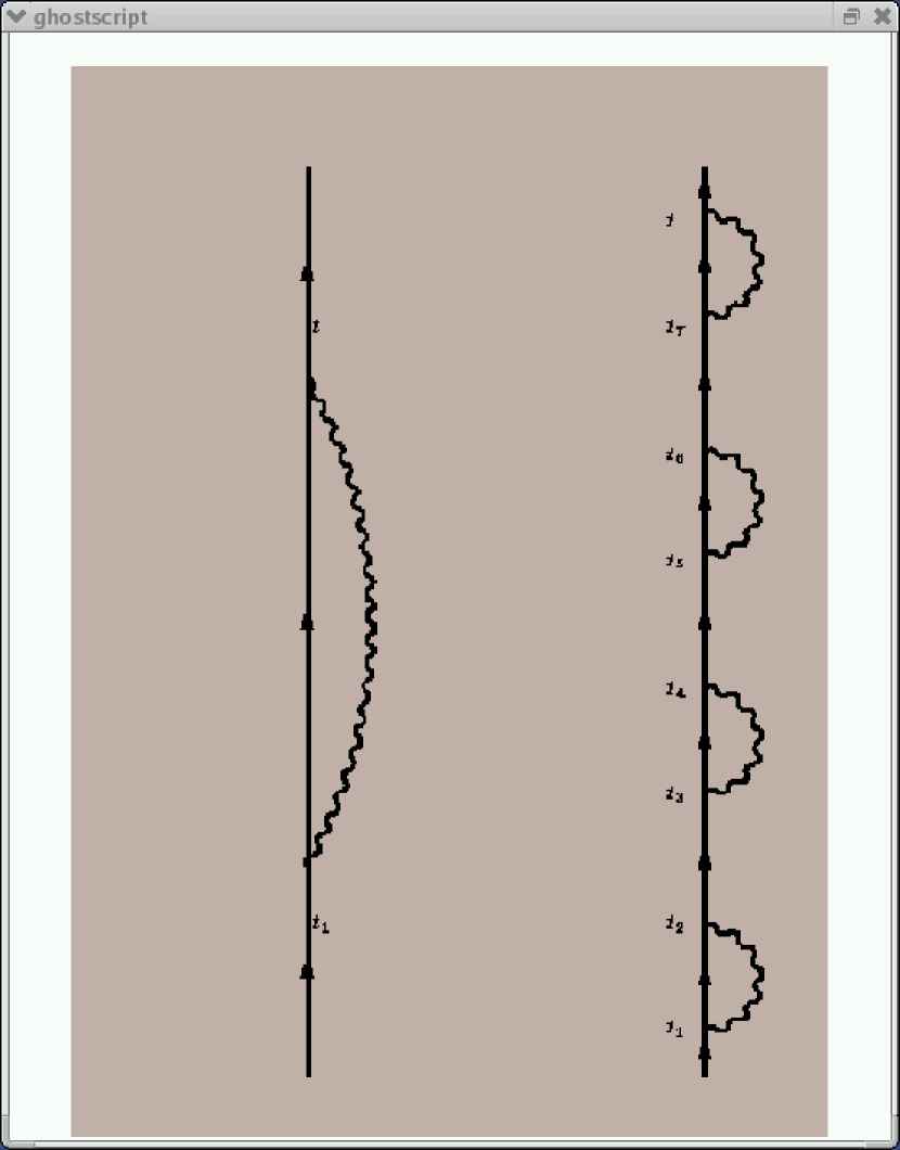
Figure 1: The left hand side of the figure shows a Feynman diagram of the process of emitting and reabsorbing a photon in the time interval $(t_{(0)},t)$ where the energy is not conserved. The electron is represented in the figure by the directed arrow and the photon by the wavy line. The right hand side of the figure shows the same process repeated four times, in a perturbative manner, over the same time interval.

As remarked, the electron is assumed to have two different states so that at $t_{1}$ and $s_{1}$ it was at the higher state 2 from which it descends to the lower state 1 through emitting a photon. Then at $t_{2}$ and $s_{2}$ it reabsorbs the photon and returns to state 2 as schematically shown at the left hand side of Figure 1. In the following we denote the higher and lower energies of the electron by $\epsilon_{2}$ and $\epsilon_{1}$ respectively and that of the photon by $w_{\lambda}$ where, due to the nonconserved energy character of the interaction, $\epsilon_{2}-\epsilon_{1}\neq w_{\lambda}$. We wish to represent the $s$ dependence of the electron and photon in the extra dimension in a similar manner as their $t$ dependence. The conventional $t$ dependence (see, for example, Chapter 7 in [24]) of an incoming electron with energy $\epsilon_{2}$ at time $t_{1}$ (before any interaction of it) is $e^{-i\epsilon_{2}t_{1}}$ and that of an outgoing electron with energy $\epsilon_{1}$ at time $t_{2}$ (after any interaction of it) is $e^{i\epsilon_{1}t_{2}}$. The $t$ dependence of the emitted photon at $t_{1}$ is [24] $e^{iw_{\lambda}t_{1}}$ and that of the reabsorbed photon at $t_{2}$ by $e^{-iw_{\lambda}t_{2}}$. Thus, according to the former discussion the $(s,t)$ dependence of the incoming electron $\phi(s,t)$ and the emitted photon $u(s,t)$ at $t_{1}$ and $s_{1}$ may be represented by

$$\phi(s_{1},t_{1})_{before\ emission}=e^{-i\epsilon_{2}t_{1}}+e^{-i\epsilon_{2}s_{1}(1-i\delta)}$$ (50)

$$u(s_{1},t_{1})_{after\ emission}=e^{iw_{\lambda}t_{1}}+e^{iw_{\lambda}s_{1}(1+i\delta)},$$

where $\delta$ is an infinitesimal satisfying $\delta\cdot\infty=\infty$, and $\delta\cdot c=0$, ($c$ is a constant) [32]. This is done so that for finite values of $s$ the dependence upon $s$, for both the electron and photon, is similar, as remarked, to the dependence upon $t$ and when $s\to\infty$, which is the equilibrium situation in the SQ theory, the terms in $s$ vanish as required. That is

$$\phi(s_{1}<\infty,t_{1})_{before\ emission}=e^{-i\epsilon_{2}t_{1}}+e^{-i\epsilon_{2}s_{1}}$$

$$\lim_{s\to\infty}\phi(s,t_{1})_{before\ emission}=e^{-i\epsilon_{2}t_{1}}$$ (51)

$$u(s_{1}<\infty,t_{1})_{after\ emission}=e^{iw_{\lambda}t_{1}}+e^{iw_{\lambda}s_{1}},\ \ \ \ \ \lim_{s\to\infty}u(s,t_{1})_{after\ emission}=e^{iw_{\lambda}t_{1}}$$

The expression for the outgoing electron at $t_{1}$ and $s_{1}$ with the lower energy $\epsilon_{1}$ (after emitting the photon) and its reduction for finite and infinite $s$ are

$$\phi(s_{1},t_{1})_{after\ emision}=e^{i\epsilon_{1}t_{1}}+e^{i\epsilon_{1}s_{1}(1+i\delta)},$$ (52)

$$\phi(s_{1}<\infty,t_{1})_{after\ emission}=e^{i\epsilon_{1}t_{1}}+e^{i\epsilon_{1}s_{1}},\ \ \ \lim_{s\to\infty}\phi(s,t_{1})_{after\ emission}=e^{i\epsilon_{1}t_{1}},$$

where the $\delta$ has the same meaning as before. Just before the reabsorption stage at $t_{2}$ and $s_{2}$ the electron and photon are represented by

$$\phi(s_{2},t_{2})_{before\ reabsorption}=e^{-i\epsilon_{1}t_{2}}+e^{-i\epsilon_{1}s_{2}(1-i\delta)}$$ (53)

$$u(s_{2},t_{2})_{before\ reabsorption}=e^{-iw_{\lambda}t_{2}}+e^{-iw_{\lambda}s_{2}(1-i\delta)}$$

Needless to remark that, according to our discussion, the former expressions reduce, for finite and infinite $s$, to

$$\phi(s_{2}<\infty,t_{2})_{before\ reabsorption}=e^{-i\epsilon_{1}t_{2}}+e^{-i\epsilon_{1}s_{2}}$$

$$\lim_{s\to\infty}\phi(s,t_{2})_{before\ reabsorption}=e^{-i\epsilon_{1}t_{2}}$$ (54)

$$u(s_{2}<\infty,t_{2})_{before\ reabsorption}=e^{-iw_{\lambda}t_{2}}+e^{-iw_{\lambda}s_{2}},\ \ \ \ \ \lim_{s\to\infty}u(s,t_{2})_{before\ reabsorption}=e^{-iw_{\lambda}t_{2}}$$

Just after the reabsorption at $s_{2}$ and $t_{2}$ the expression for the electron and its reduction for finite and infinite $s$ are

$$\phi(s_{2},t_{2})_{after\ reabsorption}=e^{i\epsilon_{2}t_{2}}+e^{i\epsilon_{2}s_{2}(1+i\delta)}$$ (55)

$$\phi(s_{2}<\infty,t_{2})_{after\ reabsorption}=e^{i\epsilon_{2}t_{2}}+e^{i\epsilon_{2}s_{2}}$$

$$\lim_{s\to\infty}\phi(s,t_{2})_{after\ reabsorption}=e^{i\epsilon_{2}t_{2}}$$

Beside the former expressions for the separate electron and photon we should take into acount also the interaction between them, that is, the emission and reabsorption of the photon by the electron. This interaction for the emission part in the extra dimension $s$, denoted $g^{em}_{\lambda_{s}}$, may be written as

$$g^{em}_{\lambda_{s}}=-\sqrt{\frac{e^{2}}{2m^{2}\hbar w_{\lambda}\epsilon_{0}}}\int\phi_{1}(s,t)u(s,t)p\phi_{2}(s,t)dV,$$ (56)

where $\phi_{2}(s,t)$, $\phi_{1}(s,t)$, denote the two energy states of the electron as given by Eqs (50)-(55) and $u(s,t)$ is the expression for the photon given by Eqs (50)-(51) and (53)-(54). The $w_{\lambda}$ and $\epsilon_{0}$ are respectively the energy of the emitted photon and the dielectric constant in vacuum. The integration is over the volume which includes also the $s$ dimension and the $p$ is the momentum operator which is represented by $p=\frac{\hbar}{i}\Delta$. The former expression for the emission interaction is suggested so that in the limit of $s\to\infty$ it reduces to the known emission interaction which does not involve the $s$ variable (see Eq (7.112) in [24]). That is,

$$\lim_{s\to\infty}g^{em}_{\lambda_{s}}=\lim_{s\to\infty}\biggl{\{}-\sqrt{\frac{e^{2}}{2m^{2}\hbar w_{\lambda}\epsilon_{0}}}\int\phi_{1}(s,t)u(s,t)p\phi_{2}(s,t)dV\biggr{\}}=$$

$$=-\sqrt{\frac{e^{2}}{2m^{2}\hbar w_{\lambda}\epsilon_{0}}}\int\lim_{s\to\infty}(\phi_{1}(s,t))\lim_{s\to\infty}(u(s,t))p\lim_{s\to\infty}(\phi_{2}(s,t))dV=$$ (57)

$$=-\sqrt{\frac{e^{2}}{2m^{2}\hbar w_{\lambda}\epsilon_{0}}}\int\phi_{1}(t)u(t)p\phi_{2}(t)dV=g^{em}_{\lambda}$$

where the last result is obtained by noting from Eqs (50)-(55) and that in the limit $s\to\infty$ the expressions for the electron and photon reduce to their known forms [24]. The interaction for the reabsorption part may be obtained by noting that the expressions for the electron and photon participating in the reabsorption interaction are obtained by taking the hermitian adjoints of the expressions for the electron and photon participating in the emission process. Thus, using the rule [28, 33] that the hermitian adjoint of the product of some expressions is the product of their adjoints in the reverse order, one may obtain the interaction for the reabsorption part, denoted $g^{re}_{\lambda_{s}}$, from that of the emission part $g^{em}_{\lambda_{s}}$ as follows

$$g^{re}_{\lambda_{s}}=\biggl{(}{g^{em}_{\lambda_{s}}\biggr{)}}\dagger=\biggl{(}{-\sqrt{\frac{e^{2}}{2m^{2}\hbar w_{\lambda}\epsilon_{0}}}\int\phi_{1}(s,t)u(s,t)p\phi_{2}(s,t)dV}\biggr{)}\dagger=$$ (58)

$$=-\sqrt{\frac{e^{2}}{2m^{2}\hbar w_{\lambda}\epsilon_{0}}}\int({\phi_{2}(s,t)})\dagger({p})\dagger({u(s,t)})\dagger({\phi_{1}(s,t)})\dagger dV$$

The reabsorption interaction reduces at the limit of $s\to\infty$, just like the emission process in Eq (57), to the known reabsorption interaction [24] which does not involve the extra $s$ variable. That is,

$$\lim_{s\to\infty}g^{re}_{\lambda_{s}}=\lim_{s\to\infty}\biggl{\{}-\sqrt{\frac{e^{2}}{2m^{2}\hbar w_{\lambda}\epsilon_{0}}}\int({\phi_{2}(s,t)})\dagger({p})\dagger({u(s,t)})\dagger({\phi_{1}(s,t)})\dagger dV\biggr{\}}=$$

$$=-\sqrt{\frac{e^{2}}{2m^{2}\hbar w_{\lambda}\epsilon_{0}}}\int\lim_{s\to\infty}({\phi_{2}(s,t)})\dagger p\lim_{s\to\infty}({u(s,t)})\dagger\lim_{s\to\infty}({\phi_{1}(s,t)})\dagger dV=$$ (59)

$$=-\sqrt{\frac{e^{2}}{2m^{2}\hbar w_{\lambda}\epsilon_{0}}}\int({\phi_{2}(t)})\dagger p({u(t)})\dagger({\phi_{1}(t)})\dagger dV=g^{re}_{\lambda}$$

Note that the whole processes of emission and reabsorption may, respectively, be read directly from Eqs (57) and (59) if one realizes that the operator $p$ in each of these equations denotes the interaction undergone by the expressions (denoting electron or (and) photon) at its right hand side which result with the expressions (also denoting electron or (and) photon) at its left hand side. Thus, in Eq (57), which describes the emission process, the $\phi_{2}(s,t)$ at the right of $p$ denotes the initial electron with the higher energy state 2 and the $\phi_{1}(s,t)u(s,t)$ at the left of $p$ are the electron with the lower energy state 1 and the emitted photon. Likewise, in Eq (59), which describes the reabsorption process, the $({u(s,t)})\dagger({\phi_{1}(s,t)})\dagger$ at the right of $p$ denotes the initial lower energy electron and the photon, before the reabsorption, and the $({\phi_{2}(s,t)})\dagger$ at the left of $p$ is the electron with the higher energy state 2 after the reabsorption.

6 The Lamb shift as a stationary state of stochastic processes in the extra dimension

Now, we must realize that the final state at $t$ and $s$ after the reabsorption of the photon, where we remain with one electron with the higher energy state 2, is the same as the initial state at $t_{(0)}$ and $s_{(0)}$ before the emission of the photon from the higher energy electron. Thus, we may write for the relevant $P^{I}$ at the end of the whole process of emission and reabsorption [24]

$$P^{I}(\psi,t,s|\psi^{(0)},t_{(0)},s_{(0)})=P^{I}(\psi^{(0)},t_{(0)},s_{(0)})+G(s,t)P^{I}(\psi^{(0)},t_{(0)},s_{(0)}),$$ (60)

where the coefficient $G(s,t)$ denotes the mentioned evolution during the $(t_{(0)},t)$ and $(s_{(0)},s)$ intervals from the initial state $P^{I}(\psi^{(0)},t_{(0)},s_{(0)})$ back to the same state. We first note that as the $(s,t)$ dependence of the states of the electron and photon were represented as sums of two terms, one involves only the $t$ term and the second only the $s$ term, so the $(s,t)$ dependence of the entire mentioned interaction of (emission$+$reabsorption) $G(s,t)$ may also be written as a sum of two separate terms, denoted $G(t)$ and $G(s)$ each of them involves only one variable. This is done, as will just be realized, so that at the equilibrium limit the $s$ term vanishes and remains only the $t$ term as is the case regarding the mentioned $(s,t)$ representation of the states of the electron and photon (see Eqs (50)-(55)).

Thus, for the $t$ dependence of the emission process one should take into account that: (1) the emission process is executed during the interval $0<t_{1}<t_{2}$ , (2) the electron before and after emission at $t_{(1)}$ is, respectively, represented by $e^{-i\epsilon_{2}t_{1}}$ and $e^{i\epsilon_{1}t_{1}}$, (3) the emitted photon at $t_{(1)}$ is given by $e^{iw_{\lambda}t_{1}}$ and (4) the emission itself is described by the interaction $g^{em}_{\lambda}$. And for the $t$ dependence of the reabsorption process one should take into account that: (1) the reabsorption process is executed during the interval $0<t_{2}<t$ , (2) the electron before and after reabsorption at $t_{(2)}$ is, respectively, represented by $e^{-i\epsilon_{1}t_{2}}$ and $e^{i\epsilon_{2}t_{2}}$, (3) the reabsorbed photon at $t_{(2)}$ is given by $e^{-iw_{\lambda}t_{2}}$ and (4) the reabsorption itself is described by the interaction $g^{re}_{\lambda}=({g^{em}_{\lambda}})\dagger$. Thus, one may write the $t$ dependence of the (emission$+$reabsorption) process $G(t)$ as

$$G(t)=g^{em}_{\lambda}\cdot({g^{em}_{\lambda}})\dagger\cdot\int_{0}^{t_{2}}\exp\biggl{(}i\bigl{(}\epsilon_{1}+w_{\lambda}-\epsilon_{2}\bigr{)}t_{1}\biggr{)}dt_{1}\cdot$$ (61)

$$\cdot\int_{0}^{t}\exp\biggl{(}i\bigl{(}\epsilon_{2}-w_{\lambda}-\epsilon_{1}\bigr{)}t_{2}\biggr{)}dt_{2}$$

Simiarly, for the $s$ dependence of the emission process one should take into account that: (1) the emission process is executed during the interval $0<s_{1}<s_{2}$ , (2) the electron before and after emission is, respectively, represented by $e^{-i\epsilon_{2}s_{1}(1-i\delta)}$ and $e^{i\epsilon_{1}s_{1}(1+i\delta)}$, (3) the emitted photon is given by $e^{iw_{\lambda}s_{1}(1+i\delta)}$ and (4) the emission itself is described by the interaction $g^{em}_{\lambda_{s}}$. And for the $s$ dependence of the reabsorption process one should take into account that: (1) the reabsorption process is executed during the interval $0<s_{2}<s$, (2) the electron before and after reabsorption is, respectively, represented by $e^{-i\epsilon_{1}s_{2}(1-i\delta)}$ and $e^{i\epsilon_{2}s_{2}(1+i\delta)}$, (3) the reabsorbed photon is given by $e^{-iw_{\lambda}s_{2}(1-i\delta)}$ and (4) the reabsorption itself is described by the interaction $g^{re}_{\lambda_{s}}=({g^{em}_{\lambda_{s}}})\dagger$. Thus, one may write the $s$ dependence of the (emission$+$reabsorption) process $G(s)$ as

$$G(s)=g^{em}_{\lambda_{s}}\cdot({g^{em}_{\lambda_{s}}})\dagger\cdot\int_{0}^{s_{2}}\exp\biggl{[}i\biggl{(}\epsilon_{1}+i\delta\bigl{(}\epsilon_{2}+\epsilon_{1}+w_{\lambda}\bigr{)}+w_{\lambda}-\epsilon_{2}\biggr{)}s_{1}\biggr{]}ds_{1}\cdot$$

$$\cdot\int_{0}^{s}\exp\biggl{[}i\biggl{(}\epsilon_{2}+i\delta\bigl{(}\epsilon_{2}+\epsilon_{1}+w_{\lambda}\bigr{)}-w_{\lambda}-\epsilon_{1}\biggr{)}s_{2}\biggr{]}ds_{2},$$ (62)

where we have set, as remarked, $s_{(0)}=t_{(0)}=0$ for both $G(t)$ and $G(s)$. The coefficient $G(t,s)$ from Eq (60) is given, as remarked, by the sum $G(t)+G(s)$ so that in the equilibrium state obtained in the limit in which all the values of $s$ are equated to each other and taken to infinity the term $G(s)$ vanishes and remains only the term $G(t)$ as should be [24]. The term $G(s)$ vanishes in the stationary state because we have already equated the initial $s_{(0)}$ to zero so for equating all the $s$’s to each other one have to set also the other values of $s$ equal to zero which obviously causes $G(s)$ from Eq (62) to vanish. Note that thus far we have discussed a single mode $\lambda$ for the emitted and reabsorbed photon which makes sense in a cavity whose closed walls are of the same order as the wavelength of the photon. But for an infinite space or a cavity with open sides one should consider a continuum of modes $\sum_{\lambda}$. Thus, considering this continuum of modes and performing the integration over $t_{1}$ and $s_{1}$ from Eqs (61)-(62) one obtains

$$G(t,s)=G(t)+Gs)=\sum_{\lambda}g^{em}_{\lambda}\cdot({g^{em}_{\lambda}})\dagger\cdot\int_{0}^{t}dt_{2}\frac{\biggl{\{}\exp\biggl{[}i(\epsilon_{1}+w_{\lambda}-\epsilon_{2})t_{2}\biggr{]}-1\biggr{\}}}{i(\epsilon_{1}+w_{\lambda}-\epsilon_{2})}\cdot$$

$$\cdot\exp\biggl{[}i(\epsilon_{2}-w_{\lambda}-\epsilon_{1})t_{2}\biggr{]}+\sum_{\lambda_{s}}g^{em}_{\lambda_{s}}\cdot({g^{em}_{\lambda_{s}}})\dagger\cdot$$ (63)

$$\cdot\int_{0}^{s}ds_{2}\frac{\biggl{\{}\exp\biggl{[}i\biggl{(}\epsilon_{1}-\epsilon_{2}+w_{\lambda}+i\delta(\epsilon_{2}+\epsilon_{1}+w_{\lambda})\biggr{)}s_{2}\biggr{]}-1\biggr{\}}}{i\biggl{(}\epsilon_{1}-\epsilon_{2}+w_{\lambda}+i\delta(\epsilon_{2}+\epsilon_{1}+w_{\lambda})\biggr{)}}\cdot$$

$$\cdot\exp\biggl{[}i\biggl{(}\epsilon_{2}-\epsilon_{1}-w_{\lambda}+i\delta\bigl{(}\epsilon_{2}+\epsilon_{1}+w_{\lambda}\bigr{)}\biggr{)}s_{2}\biggr{]}$$

Now, performing the integration over $s_{2}$ and $t_{2}$ we obtain from Eq (63)

$$G(s,t)=G(t)+G(s)=\sum_{\lambda}\frac{g^{em}_{\lambda}\cdot({g^{em}_{\lambda}})\dagger}{i\bigl{(}\epsilon_{1}+w_{\lambda}-\epsilon_{2}\bigr{)}}\biggl{\{}t-\frac{\exp\biggl{(}i\bigl{(}\epsilon_{2}-\epsilon_{1}-w_{\lambda}\bigr{)}t\biggr{)}-1}{i\bigl{(}\epsilon_{2}-\epsilon_{1}-w_{\lambda}\bigr{)}}\biggr{\}}+$$

$$+\sum_{\lambda_{s}}\frac{g^{em}_{\lambda_{s}}\cdot({g^{em}_{\lambda_{s}}})\dagger}{i\biggl{(}\epsilon_{1}-\epsilon_{2}+w_{\lambda}+i\delta\bigl{(}\epsilon_{2}+\epsilon_{1}+w_{\lambda}\bigr{)}\biggr{)}}\biggl{\{}-\frac{\exp\biggl{(}-2\delta\bigl{(}\epsilon_{2}+\epsilon_{1}+w_{\lambda}\bigr{)}s\biggr{)}-1}{2\delta\bigl{(}\epsilon_{2}+\epsilon_{1}+w_{\lambda}\bigr{)}}-$$ (64)

$$-\frac{\exp\biggl{[}i\biggl{(}\epsilon_{2}-\epsilon_{1}-w_{\lambda}+i\delta\bigl{(}\epsilon_{2}+\epsilon_{1}+w_{\lambda}\bigr{)}\biggr{)}s\biggr{]}-1}{i\biggl{(}\epsilon_{2}-\epsilon_{1}-w_{\lambda}+i\delta\bigl{(}\epsilon_{2}+\epsilon_{1}+w_{\lambda}\bigr{)}\biggr{)}}\biggr{\}}$$

One may realize that, because of the $\delta$ (see its definition after Eq (50)), the quotient $-\frac{\exp\biggl{(}-2\delta\bigl{(}\epsilon_{2}+\epsilon_{1}+w_{\lambda}\bigr{)}s\biggr{)}-1}{2\delta\bigl{(}\epsilon_{2}+\epsilon_{1}+w_{\lambda}\bigr{)}}$ in the second sum, which is of the kind $\frac{0}{0}$, may be evaluated, using L’hospital theorem [31], to obtain for it the result of $s$ so that Eq (64) becomes

$$G(s,t)=G(t)+Gs)=\sum_{\lambda}\frac{g^{em}_{\lambda}\cdot({g^{em}_{\lambda}})\dagger}{i\bigl{(}\epsilon_{1}+w_{\lambda}-\epsilon_{2}\bigr{)}}\biggl{\{}t-\frac{\exp\biggl{(}i\bigl{(}\epsilon_{2}-\epsilon_{1}-w_{\lambda}\bigr{)}t\biggr{)}-1}{i\bigl{(}\epsilon_{2}-\epsilon_{1}-w_{\lambda}\bigr{)}}\biggr{\}}+$$

$$+\sum_{\lambda_{s}}\frac{g^{em}_{\lambda_{s}}\cdot({g^{em}_{\lambda_{s}}})\dagger}{i\biggl{(}\epsilon_{1}-\epsilon_{2}+w_{\lambda}+i\delta\bigl{(}\epsilon_{2}+\epsilon_{1}+w_{\lambda}\bigr{)}\biggr{)}}\biggl{\{}s-$$ (65)

$$-\frac{\exp\biggl{[}i\biggl{(}\epsilon_{2}-\epsilon_{1}-w_{\lambda}+i\delta\bigl{(}\epsilon_{2}+\epsilon_{1}+w_{\lambda}\bigr{)}\biggr{)}s\biggr{]}-1}{i\biggl{(}\epsilon_{2}-\epsilon_{1}-w_{\lambda}+i\delta\bigl{(}\epsilon_{2}+\epsilon_{1}+w_{\lambda}\bigr{)}\biggr{)}}\biggr{\}}$$

The last expression for $G(t,s)$ contains terms which are proportional to $t$ and $s$, others which are oscillatory in these variables, and also constant terms. Thus, for large $t$ and $s$ the oscillatory as well as the constant terms may be neglected compared to $t$ and $s$ as in the analogous quantum discussion of the same process [24] (without the extra variable). That is, one may obtain for $G(s,t)$

$$G(s,t)=G(t)+G(s)=\sum_{\lambda}\frac{g^{em}_{\lambda}\cdot({g^{em}_{\lambda}})\dagger\cdot t}{i\bigl{(}\epsilon_{1}+w_{\lambda}-\epsilon_{2}\bigr{)}}+$$ (66)

$$+\sum_{\lambda_{s}}\frac{g^{em}_{\lambda_{s}}\cdot({g^{em}_{\lambda_{s}}})\dagger\cdot s}{i\biggl{(}\epsilon_{1}-\epsilon_{2}+w_{\lambda}+i\delta\bigl{(}\epsilon_{2}+\epsilon_{1}+w_{\lambda}\bigr{)}\biggr{)}}$$

Substituting from the last equation in Eq (60) one obtains

$$P^{I}(\psi,t,s|\psi^{(0)},0,0)=P^{I}(\psi^{(0)},0,0)(1+G(t,s))=$$ (67)

$$=P^{I}(\psi^{(0)},0,0)\biggl{(}1+it\Delta\epsilon_{\lambda}+is\Delta\epsilon_{\lambda_{s}}\biggr{)},$$

where $\Delta\epsilon_{\lambda}$ and $\Delta\epsilon_{\lambda_{s}}$ are

$$\Delta\epsilon_{\lambda}=\sum_{\lambda_{s}}\frac{g^{em}_{\lambda_{s}}\cdot g^{em}_{\lambda_{s}}}{\epsilon_{2}-\epsilon_{1}-w_{\lambda}},\ \ \ \Delta\epsilon_{\lambda_{s}}=\sum_{\lambda_{s}}\frac{g^{em}_{\lambda_{s}}\cdot g^{em}_{\lambda_{s}}}{\epsilon_{2}-\epsilon_{1}-w_{\lambda}-i\delta(\epsilon_{2}+\epsilon_{1}+w_{\lambda})}$$ (68)

The result in Eq (67) is only for the first-order term in Eq (49) which involves one emission and one reabsorption done over the intervals $s_{(0)},s)$, $t_{(0)},t)$. If these emission and reabsorption are repeated for each one of the many subintervals into which the former finite $s$ and $t$ intervals were subdivided so that all the higher order terms of this process ($N\to\infty$) are taken into account one obtains, analogously to the quantum analog [24] (in which the variable $s$ is absent), the result

$$P^{I}(\psi,t,s|\psi^{(0)},0,0)=P^{I}(\psi^{(0)},0,0)(1+G(t,s))=P^{I}(\psi^{(0)},0,0)\biggl{\{}1+\biggl{(}it\Delta\epsilon_{\lambda}+$$

$$+\frac{1}{2!}(it\Delta\epsilon_{\lambda})^{2}+\ldots+\frac{1}{k!}(it\Delta\epsilon_{\lambda})^{k}+\ldots\biggr{)}+\biggl{(}is\Delta\epsilon_{\lambda_{s}}+\frac{1}{2!}(it\Delta\epsilon_{\lambda_{s}})^{2}+\ldots$$ (69)

$$\ldots+\frac{1}{k!}(it\Delta\epsilon_{\lambda_{s}})^{k}+\ldots\biggr{)}\biggr{\}}=P^{I}(\psi^{(0)},0,0)\biggl{(}e^{it\Delta\epsilon_{\lambda}}+e^{is\Delta\epsilon_{\lambda_{s}}}-1\biggr{)}$$

The left hand side of Figure 1 shows a Feynman diagram [24, 32, 34] of the emission and reabsorption process performed once over the relevant $t$ interval whereas the right hand side of it shows a Feynman diagram of the fourth order term of this process over the same $t$ interval. Now, as required by the SQ theory, the stationary situations are obtained in the limit of eliminating the extra variable $s$ which is done by equating all the $s$ values to each other and taking to infinity. Thus, since, as remarked, we have equated the initial $s_{(0)}$ to zero we must equate all the other $s$ values to zero. That is, the stationary state is

$$\lim_{s\to 0}P^{I}(\psi,t,s|\psi^{(0)},0,0)=\lim_{s\to 0}P^{I}(\psi^{(0)},0,0)\biggl{(}e^{it\Delta\epsilon_{\lambda}}+e^{is\Delta\epsilon_{\lambda_{s}}}-1\biggr{)}=$$ (70)

$$=P^{I}(\psi^{(0)},0,0)e^{it\Delta\epsilon_{\lambda}}$$

The last result is the one obtained in quantum field theory [24] for the same interaction (without any extra variable). The quantity $\Delta\epsilon_{\lambda}$, given by the first of Eqs (68), has the same form also in the quantum version [24], where it is termed the energy shift. This shift have been experimentally demonstrated in the quantum field theory for the case of a real many-state particle in the famous lamb shift of the Hydrogen atom [23, 24].

Note that, as for the gravitational brainwaves case, introducing the expression of the detailed electron-photon interaction for all the subintervals of $s$ and $t$ of all the stochastic processes yields a correlation among them which truly represents, in the stationary situation, the corelation of the real interaction. That is, when all the values of $s$ are equated to each other and eliminated the equilibrium stage is obtained. One may, also, note that the elimination of the $s$ variable is fulfilled by only equating all its values to each other without having to take the infinity limit (see the discussion before Eq ($A_{14}$) in Appendix $A$).

Concluding Remarks

For the first half of this work we have used the fact that the ionic currents and charges in cerebral system radiates electric waves as may be realized by attaching electrodes to the scalp. That is, one may physically and logically assume that just as these ionic currents and charges in the brain give rise to electric waves so the masses related to these ions and charges should give rise, according to the Einstein’s field equations, to weak GW’s. From this we have proceeded to calculate the correlation among an $n$ brain ensemble in the sense of finding them at some time radiating a similar gravitational waves if they were found at an earlier time radiating other GW’s. We have used as a specific example of gravitational wave the cylindrical one which have been investigated in a thorough and intensive way (see, for example [17]).

The applied mathematical model, used for calculating the mentioned correlation, was the Parisi-Wu-Namiki SQ theory [20] which assumes a stochastic process performed in an extra dimension so that at the limit of eliminating the relevant extra variable one obtains the physical stationary state. The hypothetical stochastic process, which is governed by either the Langevin or the Fokker-Plank equation, allows a large ensemble of $n$ different variables $\psi$ which describes this process [19, 20] and represent the mentioned gravitational brainwaves radiated by the $n$ brain ensemble. Thus, we have calculated the correlation in the extra dimension among the $n$ brain ensemble and show that at the limits of (1) eliminating the relevant extra variable and (2) maximum correlation one obtains the expected result of finding all of them radiating the same cylindrical GW.

A similar and parallel discussion of the electron-photon interaction, which results in the known Lamb shift, was carried in the second half of this work. This physical example is known to have originated from vacuum fluctuations and is in effect one of the first phenomena which were found to be related to these fluctuations. Thus, it seems natural to discuss it in terms of the SQ theory in which, as mentioned, some stochastic random forces at an extra dimension generate at the equilibrium stage the known physical stationary state.

As mentioned, the mechanism which allows the reduction of the random stochastic process in the extra dimension to the known physical stationary state is the introduction of this same state in all the $N$ subintervals of all the $n$ variables. This means that once all the different $s$ values are eliminated for all the subintervals of all the variables one remains with the same introduced physical stationary state for all of them. The same mechanism may be shown to take effect not only for the assumed weak cylindrical GW’s radiated by the brain and the quantum fluctuations of the Lamb shift discussed here but also for any other physical phenomena which may be discussed by variational methods.

Appendix A APPENDIX A
Representation of the Parisi-Wu-Namiki stochastic quantization

The Parisi-Wu-Namiki SQ theory [19, 20] for any stochastic process [30] may use either the Langevin equation [21] or the Fokker-Plank one [22] as its basic starting point. For the following introductory representation of the SQ theory and in Sections II-IV we find it convenient to use the Langevin equation whereas in Sections V-VI we discuss the electron-photon interaction which results in the known Lamb shift [23] from the point of view of the Fokker-Plank equation. The stochastic process, which is assumed in the SQ theory to occur in some extra dimension $s$, is generally considered to be of the Wienner-Markoff type [30] and to be described by the $n$ variables $\psi(s,t)=\biggl{(}\psi_{1}(s,t),\psi_{2}(s,t),\ldots\psi_{(n-1)}(s,t),\psi_{n}(s,t)\biggr{)}$. This stochastic process is also characterized by the $n$ random forces $\eta(s,t)=\biggl{(}\eta_{1}(s,t),\eta_{2}(s,t),\ldots\eta_{(n-1)}(s,t),\\ \eta_{n}(s,t)\biggr{)}$ which are Gaussian white noise [30]. Thus, denoting the process related to the $i$ variable by $\psi_{i}$, where $1\leq i\leq n$, one may analyze it by taking its rate of change with respect to $s$ according to the generalized Langevin equation [21]

$$\frac{\partial\psi_{i}(s,t,r)}{\partial s}=K_{i}(\psi(s,t,r))+\eta_{i}(s,t,r),\ \ \ \ \ \ \ i=1,2,\ldots n, A_{1}$$ ()

where $n$ denotes the remarked $n$-member ensemble of variables and $\eta_{i}$ denotes stochatic process related to the variable $\psi_{i}$. The variables $\psi_{i}$ depends upon $s$ and upon the spatial variable $r$ and the time $t$. The $K_{i}$ are given in the SQ theory by [19, 20]

$$K_{i}(\psi(s,t,r))=-(\frac{\delta S_{i}[\psi]}{\delta\psi})_{\psi=\psi(s,t,r)}, A_{2}$$ ()

where $S_{i}$ are the actions $S_{i}=\int\int drdtL_{i}(\psi,\dot{\psi})$ and $L_{i}$ are the Lagrangians. For properly discussing the “evolution” of the related process $\psi_{i}$ one, generally, subdivides the $t$ and $s$ intervals $(t_{(0)},t)$, $(s_{(0)},s)$ into $N$ subintervals $(t_{(0)},t_{1})$, $(t_{1},t_{2})$, …$(t_{N-1},t)$ and $(s_{(0)},s_{1})$, $(s_{1},s_{2})$, …$(s_{N-1},s)$. We assume that the Langevin Eq ($A_{1}$) is satisfied for each member of the ensemble of variables at each subinterval with the following Gaussian constraints [20]

$$<\!\eta^{(k)}_{i}(t_{k},s_{k})\!>=0,\ \ \ <\!\eta^{(k)}_{i}(t_{k},s_{k})\eta^{(k)}_{j}(\grave{t}_{k},\grave{s}_{k})\!>=2\alpha\delta_{ij}\delta(t_{k}-\grave{t}_{k})\delta(s_{k}-\grave{s}_{k}), A_{3}$$ ()

where the angular brackets denote an ensemble average with the Gaussian distribution, the $k$ superscript denotes the $k$ subinterval from the $N$ available and the $i$, $j$ refer to the mentioned $n$ variables where $n\geq i,j\geq 1$. Note that both intervals $(t_{(0)},t)$, $(s_{(0)},s)$ of each one of the $n$ variables are subdivided, as mentioned, into $N$ subintervals. The $\alpha$ from Eq ($A_{3}$) have different meanings which depend upon the involved process and the context in which Eqs ($A_{1}$) and ($A_{3}$) are used. Thus, in the classical regime $\alpha$ is [20] $\alpha=\frac{k_{\beta}T}{f}$, where $k_{\beta}$, $T$, and $f$ are respectively the Boltzman constant, the temperature in Kelvin units and the relevant friction coefficient. In the quantum regime $\alpha$ is identified [20] with the Plank constant $\hbar$. We note that using Eqs ($A_{1}$)-($A_{3}$) enables one [20] to discuss a large number of different classical and quantum phenomena. It has been shown [20] that the right hand side of Eq ($A_{3}$) may be derived from the following Gaussian distribution law [20]

$$P_{i}(y)dy_{i}=\frac{1}{\sqrt{2\pi(<\!\eta^{(k)}_{i}\!>)^{2}}}\exp(-\frac{(y^{(k)}_{i})^{2}}{2(<\!\eta^{(k)}_{i}\!>)^{2}})dy_{i}, A_{4}$$ ()

which is the probability density for the variable $\psi_{i}$ and for the subintervals $(s_{(k-1)},s_{k})$, $(t_{(k-1)},t_{k})$ to have a value of $\eta^{(k)}_{i}$ in $(y^{(k)}_{i},y^{(k)}_{i}+dy_{i})$ [20], where

$$y^{(k)}_{i}=\frac{\partial\psi^{(k)}_{i}(s,t,x)}{\partial s}-K_{i}(\psi^{(k)}_{i}(s,t,x)) A_{5}$$ ()

For the $n$ variables one may write Eq ($A_{4}$) for the subintervals $(s_{(k-1)},s_{k})$, $(t_{(k-1)},t_{k})$ as

$$P_{ij...}(y)dy=\exp(-\sum_{i=1}^{n}\frac{(y^{(k)}_{i})^{2}}{2(<\!\eta^{(k)}_{i}\!>)^{2}})\prod_{i=1}^{n}\frac{dy_{i}}{\sqrt{2\pi(<\!\eta^{(k)}_{i}\!>)^{2}}}, A_{6}$$ ()

which is the probability density for the $n$ variables $\psi_{i}\ \ 1\leq i\leq n$ to have a value of $\eta^{(k)}_{i}$ in $(y^{(k)}_{i},y^{(k)}_{i}+dy_{i})$ where $dy=\prod_{i}dy_{i}$. The angular brackets are product over any two variables as given in Eq ($A_{3}$). We note in this context that the general correlation $<\!\eta_{i}\eta_{j}\ldots\eta_{m}\eta_{n}\!>$ is expressed in terms of $<\!\eta_{i}\eta_{j}\!>$ by [20]

$$<\!\eta_{i}\eta_{j}\ldots\eta_{m}\eta_{n}\!>=\left\{\begin{array}[]{ll}0&{\rm for\ odd\ number\ of\eta^{\prime}s}\\ \sum<\!\eta_{i}\eta_{j}\!><\!\eta_{m}\eta_{n}\!>\ldots&{\rm for\ even\ number\ of\ \eta^{\prime}s}\end{array}\right.$$ (73)

where the sum is taken over every possible pair of $\eta^{\prime}s$. For the whole intervals $(s_{(0)},s)$, $(t_{(0)},t)$, which as mentioned were each subdivided into $N$ subintervals, one may generalize Eq ($A_{6}$) as

$$P_{ij...}(y)dy=\exp(-\sum_{i=1}^{n}\sum_{k=1}^{N}\frac{(y^{(k)}_{i})^{2}}{2(<\!\eta^{(k)}_{i}\!>)^{2}})\prod_{i=1}^{n}\prod_{k=1}^{N}\frac{dy^{(k)}_{i}}{\sqrt{2\pi(<\!\eta_{i}^{(k)}\!>)^{2}}}, A_{8}$$ ()

where now the $dy$ at the left is $dy=\prod_{i}\prod_{k}dy^{(k)}_{i}$. Note that Eqs ($A_{4}$), ($A_{6}$) and ($A_{8}$) denote probability densities as realized from the $dy$ at the left hand sides of these equations. In order to find the probabilities themselves one have to integrate the right hand sides of these equations over the appropriate variables. Thus, using Eqs ($A_{1}$), ($A_{3}$) and ($A_{5}$) one may write Eq ($A_{4}$) in a more informative way as

$$P_{i}\bigl{(}\psi^{(k)}_{i},t_{k},s_{k}|\psi^{(k-1)}_{i},t_{(k-1)},s_{(k-1)}\bigr{)}= A_{9}$$ ()

$$=\int d\psi_{i}^{(k)}\frac{1}{\sqrt{2\pi(2\alpha)}}\exp\biggl{\{}-\frac{\biggl{(}\frac{\psi^{(k)}_{i}-\psi^{(k-1)}_{i}}{(s_{k}-s_{(k-1)})}-K_{i}(\psi_{i}^{(k-1)})\biggr{)}^{2}}{2(2\alpha)}\biggr{\}}dy,$$

where we have approximated $\frac{\partial\psi^{(k)}_{i}(s,t,x)}{\partial s}\approx\frac{\psi_{i}^{(k)}-\psi_{i}^{(k-1)}}{(s_{k}-s_{(k-1)})}$. The $P_{i}\bigl{(}\psi_{i}^{(k)},t_{k},s_{k}|\psi_{i}^{(k-1)},t_{(k-1)},s_{(k-1)}\bigr{)}$ of Eq ($A_{9}$) is the conditional probability to find the variable $\psi_{i}$ at $t_{k}$ and $s_{k}$ with the configuration $\psi^{(k)}_{i}$ if at $t_{(k-1)}$ and $s_{(k-1)}$ it has the configuration $\psi^{(k-1)}_{i}$. Since it involves the same variable it may be termed autocorrelation of $\psi_{(i)}$ over the subintervals $(s_{(k-1)},s_{(k)})$, $(t_{(k-1)},t_{(k)})$. In a similar manner one may write Eq ($A_{9}$) for the whole ensemble of $n$ variables in the subintervals $(s_{(k-1)},s_{k})$ and $(t_{(k-1)},t_{k})$ as

$$P_{ij...}\bigl{(}\psi_{(n)}^{(k)},t_{k},s_{k}|\psi_{(0)}^{(k-1)},t_{(k-1)},s_{(k-1)}\bigr{)}=\int\cdots\int\exp\biggl{\{}-\sum_{i}\frac{\biggl{(}\frac{\psi_{i}^{(k)}-\psi_{i}^{(k-1)}}{(s_{k}-s_{(k-1)})}-K_{i}(\psi_{i}^{(k-1)})\biggr{)}^{2}}{2(2\alpha)}\biggr{\}}\cdot$$

$$\cdot\prod_{(i=1)}^{(i=n)}\frac{d\psi_{(i)}^{(k)}}{\sqrt{2\pi(2\alpha)}} A_{10}$$ ()

And the conditional probability over the whole intervals $(s_{(0)},s)$ and $(t_{(0)},t)$ may similarly be obtained by adding other factors and sums over the remaining $(N-1)$ subintervals. If one assume $N$ to be very large, and therefore the length of each subinterval to be very small, one may use Feynman path integral [34] as follows

$$P_{ij...}\bigl{(}\psi,t,s|\psi_{(0)},t_{(0)},s_{(0)}\bigr{)}=\lim_{N\to\infty}C\int\ldots\int\exp\biggl{\{}-\sum_{i=1}^{n}\sum_{k=1}^{N}\frac{\biggl{(}\frac{\psi_{i}^{(k)}-\psi_{i}^{(k-1)}}{(s_{k}-s_{(k-1)})}-K_{i}(\psi_{i}^{(k-1)})\biggr{)}^{2}}{2(2\alpha)}\biggr{\}}\cdot$$

$$\cdot\prod_{i=1}^{n}\prod_{k=1}^{N}\biggl{(}\frac{d\psi_{(i)}^{(k)}}{\sqrt{2\pi(2\alpha)}}\biggr{)}, A_{11}$$ ()

where $C$ is a normalization constant. The former formula may equivalently be written as [20]

$$P\bigl{(}\psi,t,s|\psi_{(0)},t_{(0)},s_{0}\bigr{)}=C\int\cdots\int\cdots\int P\bigl{(}\psi_{(n)}^{N},t_{N},s_{N}|\psi_{(0)}^{(N-1)},t_{(N-1)},s_{(N-1)}\bigr{)}\cdots A_{12}$$ ()

$$\cdots P\bigl{(}\psi_{(n)}^{k},t_{k},s_{k}|\psi_{(0)}^{k-1},t_{(k-1)},s_{(k-1)}\bigr{)}\cdots P\bigl{(}\psi_{(n)}^{1},t_{1},s_{1}|\psi_{(0)}^{0},t_{(0)},s_{0}\bigr{)}d\psi^{N}\cdots d\psi^{k}\cdots d\psi^{1},$$

where each $P$ at the right is essentially of the form of Eq ($A_{10}$) and the integrals are over the $N$ subintervals. The last equation, which is the conditional probability to find the ensemble of $n$ variables at $t$ and $s$ with the configuration $\psi$ if at $t_{(0)}$ and $s_{(0)}$ they have the configuration $\psi_{(0)}$, is also equivalent [20] to the Green’s functions $\Delta_{ij\ldots}(t_{(0)},s_{(0)},t_{1},s_{1},\ldots)$ which determine the correlation among the members of the ensemble [20]. This function, as defined in [20], is

$$\Delta_{ij\ldots}(t_{(0)},s_{(0)},t_{1},s_{1},\ldots)=<\!\psi_{i}(t_{(0)},s_{(0)})\psi_{j}(t_{1},s_{1})\ldots\!>= A_{13}$$ ()

$$=C\int D\psi(t,s)\psi_{i}(t_{(0)},s_{(0)})\psi_{j}(t_{1},s_{1})\ldots\exp(-\frac{S_{i}(\psi(t,s))}{\alpha}),$$

where $S_{i}$ are the actions $S_{i}=\int dsL_{i}(\psi,\dot{\psi})$, $C$ is a normalization constant, and $D\psi(t,s)=\prod_{i=1}^{i=n}d\psi_{i}(t,s)$. As seen from the last equation the $\Delta_{ij\ldots}(t_{(0)},s_{(0)},t_{1},s_{1}\ldots)$ were expressed as path integrals [34] where the quantum feynman measure $e^{\frac{iS(\psi)}{\hbar}}$ is replaced in Eq ($A_{13}$) and in the following Eq ($A_{14}$) by $e^{-\frac{S(q)}{\alpha}}$ as required for the classical path integrals [20, 35].

It can be seen that when the $s$’s are different for the members of the ensemble so that each have its specific $S_{i}(\psi(s_{i},t))$, $K_{i}(\psi(s_{i},t))$, and $\eta_{i}(s_{i},t)$ the correlation in ($A_{13}$) is obviously zero. Thus, in order to have a nonzero value for the probability to find a large part of the ensemble of variables having the same or similar forms we have to consider the stationary configuration where, as remarked, all the $s$ values are equated to each other and taken to infinity. For that matter we take account of the fact that the dependence upon $s$ and $t$ is through $\psi$ so this ensures [20] that this dependence is expressed through the $s$ and $t$ differences. For example, referring to the members $i$ and $j$ the correlation between them is $\Delta_{ij}(t_{i}-t_{j},s_{i}-s_{j})$, so that for eliminating the $s$ variable from the correlation function one equates all these different $s$’s to each other. We, thus, obtain the following stationary equilibrium correlation [20]

$$\Delta_{ij\ldots}(t_{(0)},s_{(0)},\ldots)_{st}=<\!\psi_{i}(t_{(0)},s_{(0)})\psi_{j}(t_{1},s_{1})\ldots\!>_{st}=C\int D\psi(t)\psi_{i}(t_{(0)})\psi_{j}(t_{1})\ldots A_{14}$$ ()

$$\ldots\exp(-\frac{S(\psi)}{\alpha}),$$

where the suffix of $st$ denotes the stationary configuration. In other words, the equilibrium correlation in our case is obtained when all the different $s$ values are equated to each other and taken to infinity in which case one remains with the known stationary result.

Thus, if all the members of the ensemble of variables have similar actions $S$ (in which the $s$ values are equated to each other) one finds with a large probability these members, in the later equilibrium stage, with the same result. That is, introducing the same similar actions into the corresponding path integrals one finds this mentioned large probability. This has been expicitly shown in Section IV for the cylindrical gravitational wave and in Sections V-VI for the Lamb shift case.

Appendix B APPENDIX B
Derivation of the correlation expression from Eq (39)

We, now, derive the expression for the correlation from Eq (39). For that we may use Eq ($A_{12}$) of Appendix $A$ in which we substistute for the $P$’s from Eqs ($A_{9}$)-($A_{10}$). As noted in Appendix $A$ the correlation is calculated not only among the ensemble of $n$ variables but also for each of the $N$ subintervals into which the finite $t$ and $s$ intervals are divided. Thus, assuming, as noted in Appendix $A$, that $N$ is very large we may use the Feynman path integral of Eq ($A_{11}$) and write this correlation as

$$P_{ij...}\bigl{(}\psi,t,s|\psi_{(0)},t_{(0)},s_{(0)}\bigr{)}=C\int_{-\infty}^{\infty}\ldots\int_{-\infty}^{\infty}\ldots\int_{-\infty}^{\infty}\exp\biggl{\{}-\sum_{k=1}^{N}\sum_{i=1}^{n}\frac{1}{4\alpha(s_{k}-s_{(k-1)})^{2}}\biggl{(}\psi_{i}^{(k)}-$$

$$-\psi_{(i-1)}^{(k)}-K_{i}(\psi_{(i-1)}^{(k)})(s_{k}-s_{(k-1)})\biggr{)}^{2}\biggr{\}}\prod_{k=1}^{k=N}\prod_{i=1}^{i=(n-1)}\frac{d\psi^{k}_{i}}{\sqrt{2\pi\bigl{(}2\alpha\bigr{)}}} B_{1}$$ ()

where $C$ is a normalization constant to be determined later from $\int P_{ij...}\bigl{(}\psi,t,s|\psi^{0},t_{(0)},s_{(0)}\bigr{)}d\psi=1$. Note that in the exponent of Eq ($B_{1}$), in contrast to that of Eq ($A_{11}$) in Appendix $A$, the sum over $i$ precedes that over $k$ and, therefore, the squared expression involves the variables $\psi_{(i)}^{(k)}$, $\psi_{(i-1)}^{(k)}$ etc (instead of $\psi_{(i)}^{(k)}$, $\psi_{(i)}^{(k-1)}$ of ($A_{11}$)). Note also that the number of integrals are $N\times(n-1)$ over the $N$ subintervals and $(n-1)$ variables which is related to the fact that the suffix $i$ in the exponent is summed from $i=1$ to $i=n$ whereas the $i$ in the differentials outside the exponent is summed up to $i=n-1$ (compare with equation (4.4 in [20]). The reason for this is that each $\psi_{(i)}^{(k)}$, except for $i=0$ and $i=n$, with superscript $k$ and suffix $i$ appears in two consecutive squared expressions of the sum over $i$ so for calculating the correlation for the observer $i$ over the subinterval $(s_{k}-s_{(k-1)})$ one has to solve the following integral which is related to $\psi_{(i)}^{(k)}$.

$$P_{i}\bigl{(}\psi^{(k)}_{i},t_{(k)},s_{(k)}|\psi^{(k)}_{(i-1)},t_{(k-1)},s_{(k-1)}\bigr{)}=$$

$$=\int_{-\infty}^{\infty}\exp\biggl{\{}-\biggl{[}\frac{\biggl{(}\psi_{i}^{(k)}-\psi_{(i-1)}^{(k)}-K_{i}(\psi_{(i-1)}^{(k)})(s_{k}-s_{(k-1)})\biggr{)}^{2}}{2(2\alpha)\bigl{(}s_{k}-s_{(k-1)}\bigr{)}^{2}}+ B_{2}$$ ()

$$+\frac{\biggl{(}\psi_{(i+1)}^{(k)}-\psi_{i}^{(k)}-K_{i}(\psi_{i}^{(k)})(s_{(k)}-s_{(k-1)})\biggr{)}^{2}}{2(2\alpha)\bigl{(}s_{(k)}-s_{(k-1)}\bigr{)}^{2}}\biggr{]}\biggr{\}}\frac{d\psi^{(k)}_{i}}{\sqrt{2\pi(2\alpha)}}$$

The solution of this integral involves the substitution for $K_{i}(\psi_{(i-1)}^{(k)})$ and $K_{i}(\psi_{i}^{(k)})$ from Eqs (32) and (36) so that one may write the two squared expressions of Eq ($B_{2}$) as

$$\frac{\biggl{(}\psi_{i}^{(k)}-\psi_{(i-1)}^{(k)}-K_{i}(\psi_{(i-1)}^{(k)})(s_{k}-s_{(k-1)})^{2}\biggr{)}^{2}}{2(2\alpha)\bigl{(}s_{(k)}-s_{(k-1)}\bigr{)}}=\frac{1}{2(2\alpha)\bigl{(}s_{(k)}-s_{(k-1)}\bigr{)}^{2}}\biggl{[}\psi_{i}^{(k)}-$$

$$-\psi_{(i-1)}^{(k)}-2\pi\biggl{(}B_{1}(R,t)\psi^{(k)}_{(i-1)}-B_{2}(R,t)-iB_{3}(R,t)\biggr{)}(s_{k}-s_{(k-1)})\biggr{]}^{2} B_{3}$$ ()

$$\frac{\biggl{(}\psi_{(i+1)}^{(k)}-\psi_{i}^{(k)}-K_{i}(\psi_{i}^{(k)})(s_{(k)}-s_{(k-1)})\biggr{)}^{2}}{2(2\alpha)\bigl{(}s_{(k)}-s_{(k-1)}\bigr{)}^{2}}=\frac{1}{2(2\alpha)\bigl{(}s_{(k)}-s_{(k-1)}\bigr{)}^{2}}\biggl{[}\psi_{(i+1)}^{(k)}-$$

$$-\psi_{i}^{(k)}-2\pi\biggl{(}B_{1}(R,t)\psi^{(k)}_{i}-B_{2}(R,t)-iB_{3}(R,t)\biggr{)}(s_{(k)}-s_{(k-1)})\biggr{]}^{2}$$

In order to deal with manageable expressions we first assume that in the limit of large $N$ and $n$ the subintervals over $t$ and $s$ are equal so that one may write for any integral $k$

$$\Delta s_{k}=(s_{k}-s_{(k-1)})=\Delta s_{(k+1)}=(s_{(k+1)}-s_{(k)})=\Delta s B_{4}$$ ()

$$\Delta t_{k}=(t_{k}-t_{(k-1)})=\Delta t_{(k+1)}=(t_{(k+1)}-t_{(k)})=\Delta t$$

We, now, define the following expressions

$$a_{1}=(1+2\pi B_{1}\Delta s)^{2},\ \ \ \ a_{2}=2\pi\Delta s(B_{2}+iB_{3}) B_{5}$$ ()

Using Eqs ($B_{3}$)-($B_{5}$) one may write the two squared terms of Eq ($B_{2}$) as

$$\frac{\biggl{(}\psi_{i}^{(k)}-\psi_{(i-1)}^{(k)}-K_{i}(\psi_{(i-1)}^{(k)})(s_{k}-s_{(k-1)})\biggr{)}^{2}}{2(2\alpha)\bigl{(}s_{(k)}-s_{(k-1)}\bigr{)}^{2}}+\frac{\biggl{(}\psi_{(i+1)}^{(k)}-\psi_{i}^{(k)}-K_{i}(\psi_{i}^{(k)})(s_{(k)}-s_{(k-1)})\biggr{)}^{2}}{2(2\alpha)\bigl{(}s_{(k)}-s_{(k-1)}\bigr{)}^{2}}=$$

$$=\frac{1}{4\alpha(\Delta s)^{2}}\biggl{\{}\biggl{(}\psi^{(k)}_{i}-\sqrt{a_{1}}\psi^{(k)}_{(i-1)}+a_{2}\biggr{)}^{2}+\biggl{(}\psi^{(k)}_{(i+1)}-\sqrt{a_{1}}\psi^{(k)}_{i}+a_{2}\biggr{)}^{2}\biggr{\}}= B_{6}$$ ()

$$=\frac{1}{4\alpha(\Delta s)^{2}}\biggl{\{}(\psi^{k}_{i})^{2}+a_{1}(\psi^{(k)}_{(i-1)})^{2}-2\sqrt{a_{1}}\psi^{(k)}_{i}\psi^{(k)}_{(i-1)}+2a_{2}\psi^{(k)}_{i}-2a_{2}\sqrt{a_{1}}\psi^{(k)}_{(i-1)}+$$

$$+(\psi^{(k)}_{(i+1)})^{2}+a_{1}(\psi^{(k)}_{i})^{2}-2\sqrt{a_{1}}\psi^{(k)}_{(i+1)}\psi^{(k)}_{i}+2a_{2}\psi^{(k)}_{(i+1)}-2a_{2}\sqrt{a_{1}}\psi^{(k)}_{i}+2a_{2}^{2}\biggr{\}}$$

The last result is now substituted for the two squared terms of Eq ($B_{2}$) and the integral over $\psi^{k}_{i}$ may be solved by using the following integral [27]

$$\int_{-\infty}^{\infty}dx\exp\bigl{(}-\bigl{(}ax^{2}+bx+c\bigr{)}\bigr{)}=\sqrt{\frac{\pi}{a}}\exp\bigl{(}\frac{(b^{2}-4ac)}{4a}\bigr{)} B_{7}$$ ()

Thus, using Eq ($B_{6}$), one may find the appropriate coefficients $a_{\psi^{k}_{i}}$, $b_{\psi^{k}_{i}}$ and $c_{\psi^{k}_{i}}$, related to $\psi^{k}_{i}$, to be substituted in the integral ($B_{2}$) as follows

$$a_{\psi^{k}_{i}}=\frac{(1+a_{1})}{4\alpha(\Delta s)^{2}},\ \ \ \ \ b_{\psi^{k}_{i}}=\frac{\biggl{(}2a_{2}\bigl{(}1-\sqrt{a_{1}}\bigr{)}-2\sqrt{a_{1}}\bigl{(}\psi^{(k)}_{(i-1)}+\psi^{(k)}_{(i+1)}\bigr{)}\biggr{)}}{4\alpha(\Delta s)^{2}} B_{8}$$ ()

$$c_{\psi^{k}_{i}}=\frac{\biggl{[}(\psi^{(k)}_{(i+1)})^{2}+a_{1}(\psi^{(k)}_{(i-1)})^{2}+2a_{2}\biggl{(}a_{2}+\psi^{(k)}_{(i+1)}-\sqrt{a_{1}}\psi^{(k)}_{(i-1)}\biggr{)}\biggr{]}}{4\alpha(\Delta s)^{2}}$$

Using the last expressions for the coefficients $a_{\psi^{k}_{i}}$, $b_{\psi^{k}_{i}}$ and $c_{\psi^{k}_{i}}$ one may realize, after some calculations, that they satisfy the following relation

$$\frac{b^{2}_{\psi^{k}_{i}}-4a_{\psi^{k}_{i}}c_{\psi^{k}_{i}}}{4a_{\psi^{k}_{i}}}=-\frac{1}{4(1+a_{1})\alpha(\Delta s)^{2}}\biggl{(}\bigl{(}\psi^{(k)}_{(i+1)}-a_{1}\psi^{(k)}_{(i-1)}\bigr{)}+a_{2}\bigl{(}1+\sqrt{a_{1}}\bigr{)}\biggr{)}^{2} B_{9}$$ ()

Thus, using the former discussion and, especially, the integral ($B_{7}$) one is able to solve the integral from Eq ($B_{2}$) and write it as

$$P_{i}\bigl{(}\psi^{(k)}_{(i+1)},t_{(k)},s_{(k)}|\psi^{(k)}_{(i-1)},t_{(k-1)},s_{(k-1)}\bigr{)}=$$

$$=\int_{-\infty}^{\infty}\frac{d\psi^{(k)}_{i}}{\sqrt{2\pi(2\alpha)}}\exp\biggl{[}-\biggl{(}a_{\psi^{(k)}_{i}}(\psi^{(k)}_{i})^{2}+b_{\psi^{(k)}_{i}}\psi^{(k)}_{i}+c_{\psi^{(k)}_{i}}\biggr{)}\biggl{]}=\frac{1}{\sqrt{4\alpha a_{\psi^{k}_{i}}}}\cdot B_{10}$$ ()

$$\cdot\exp\biggl{(}\frac{b^{2}_{\psi^{k}_{i}}-4a_{\psi^{k}_{i}}c_{\psi^{k}_{i}}}{4a_{\psi^{k}_{i}}}\biggr{)}=\frac{\Delta s}{\sqrt{(1+a_{1})}}\exp\biggl{\{}-\biggl{[}\frac{1}{4(1+a_{1})\alpha(\Delta s)^{2}}\biggl{(}\bigl{(}\psi^{(k)}_{(i+1)}-$$

$$-a_{1}\psi^{(k)}_{(i-1)}\bigr{)}+a_{2}\bigl{(}1+\sqrt{a_{1}}\bigr{)}\biggr{)}^{2}\biggr{]}\biggr{\}}$$

The last result is the correlation for the variable $\psi_{(i)}$ over the subinterval $(s_{k}-s_{(k-1)})$ and it means the conditional probability to find this variable at $s=s_{(k)}$ and $t=t_{(k)}$ at the state $\psi_{(i+1)}^{(k)}$ if at $s=s_{(k-1)}$ and $t=t_{(k-1)}$ it was at the state $\psi_{(i-1)}^{(k)}$. Note that the superscript of the variable $\psi_{(i-1)}$ at the beginning of the subintervals $s_{(k-1)}$ and $t_{(k-1)}$ is the same as that at the end of it, i.e., $k$. If one wish to find the correlation of the two variables $\psi_{(i)}$ and $\psi_{(i+1)}$ for the same subinterval $\Delta s$ then he has to add to the last result another squared term from the general relation ($B_{1}$) and perform the required integration over $\psi^{(k)}_{(i+1)}$ as follows

$$P_{i,(i+1)}\bigl{(}\psi^{(k)}_{(i+2)},t_{(k)},s_{(k)}|\psi^{(k)}_{(i-1)},t_{(k-1)},s_{(k-1)}\bigr{)}=$$

$$=\frac{\Delta s}{\sqrt{(1+a_{1})}}\int_{-\infty}^{\infty}\exp\biggl{\{}-\biggl{[}\frac{1}{4(1+a_{1})\alpha(\Delta s)^{2}}\biggl{\{}\biggl{(}\bigl{(}\psi^{(k)}_{(i+1)}-a_{1}\psi^{(k)}_{(i-1)}\bigr{)}+a_{2}\bigl{(}1+\sqrt{a_{1}}\bigr{)}\biggr{)}^{2}+$$

$$+\biggl{(}\psi_{(i+2)}^{(k)}-\psi_{(i+1)}^{(k)}-K_{i}(\psi_{(i+1)}^{(k)})\Delta s\biggr{)}^{2}(1+a_{1})\biggr{\}}\biggr{]}\biggr{\}}\frac{d\psi^{(k)}_{(i+1)}}{\sqrt{2\pi(2\alpha)}} B_{11}$$ ()

In this case the corresponding $a_{\psi^{(k)}_{(i+1)}}$, $b_{\psi^{(k)}_{(i+1)}}$ and $c_{\psi^{(k)}_{(i+1)}}$ are

$$a_{\psi^{(k)}_{(i+1)}}=\frac{\bigl{(}1+a_{1}+a^{2}_{1})\bigr{)}}{2(2\alpha)(\Delta s)^{2}},$$

$$b_{\psi^{(k)}_{(i+1)}}=\frac{\biggl{(}2a_{2}\bigl{(}1+\sqrt{a_{1}}\bigr{)}-2a_{1}\psi^{(k)}_{(i-1)}-(1+a_{1})\biggl{(}2\sqrt{a_{1}}\psi^{(k)}_{(i+2)}+2a_{2}\sqrt{a_{1}}\biggr{)}}{2(2\alpha)(\Delta s)^{2}} B_{12}$$ ()

$$c_{\psi^{(k)}_{(i+1)}}=\frac{\biggl{(}a_{1}^{2}(\psi^{(k)}_{(i-1)})^{2}+a_{2}^{2}(1+\sqrt{a_{1}})^{2}-2a_{1}a_{2}(1+\sqrt{a_{1}})\psi^{(k)}_{(i-1)}+(1+a_{1})\bigl{(}\psi^{(k)}_{(i+2)}+a_{2}\bigr{)}^{2}\biggr{)}}{2(2\alpha)(\Delta s)^{2}}$$

Thus, using the last equations and the integral from Eq ($B_{7}$) one may write the correlation from Eq ($B_{11}$) as

$$P_{i}\bigl{(}\psi^{(k)}_{(i+2)},t_{(k)},s_{(k)}|\psi^{(k)}_{(i-1)},t_{(k-1)},s_{(k-1)}\bigr{)}= B_{13}$$ ()

$$=\frac{(\Delta s)^{2}}{\sqrt{(1+a_{1})\bigl{(}1+a_{1}+a_{1}^{2}\bigr{)}}}\exp\biggl{\{}-\biggl{[}\frac{\biggl{(}\psi^{(k)}_{(i+2)}-a_{1}\sqrt{a_{1}}\psi^{(k)}_{(i-1)}+a_{2}\bigl{(}1+\sqrt{a_{1}}+(\sqrt{a_{1}})^{2}\bigr{)}\biggr{)}^{2}}{4\alpha(\Delta s)^{2}\bigl{(}1+a_{1}+a_{1}^{2}\bigr{)}}\biggr{]}\biggr{\}}$$

Using the results of Eq ($B_{10}$) for the observer $i$ one may realize that the correlation from Eq ($B_{13}$) means the conditional probability to find at $s=s_{(k)}$ and $t=t_{(k)}$ the two variables $\psi_{(i)}$ and $\psi_{(i+1)}$ at the respective states of $\psi_{(i+1)}^{(k)}$ and $\psi_{(i+2)}^{(k)}$ if at $s=s_{(k-1)}$ and $t=t_{(k-1)}$ they were at the states $\psi_{(i-1)}^{(k)}$, $\psi_{(i)}^{(k)}$. As remarked after Eq ($B_{10}$) the superscripts of the variables $\psi_{(i-1)}^{(k)}$, $\psi_{(i)}^{(k)}$ at the beginning of the subintervals $s_{(k-1)}$ and $t_{(k-1)}$ are the same as that at the end of it, i.e., $k$. One may, now, realize that the correlation of the $n$ observers $i,j,l...$ over the subinterval $(s_{(k-1)},s_{(k)})$ may be obtained from the results of Eqs ($B_{10}$), ($B_{13}$) and from Eq ($B_{1}$) as

$$P_{i,j,l...}\bigl{(}\psi^{(k)}_{(n)},t_{(k)},s_{(k)}|\psi^{k}_{0},t_{(k-1)},s_{(k-1)}\bigr{)}=\frac{(\Delta s)^{(n-1)}}{\sqrt{\prod_{j=1}^{j=(n-1)}(\sum_{m=0}^{m=j}a_{1}^{m})}}\cdot$$

$$\cdot\exp\biggl{\{}-\frac{1}{4\alpha(\Delta s)^{2}\sum_{p=0}^{p=(n-1)}a_{1}^{p}}\biggl{(}\psi_{n}^{(k)}-(\sqrt{a_{1}})^{n+1}\psi_{0}^{(k)}+a_{2}\sum_{r=0}^{r=n+1}(\sqrt{a_{1}})^{r}\biggr{)}^{2}\biggr{\}}, B_{14}$$ ()

The last correlation means the conditional probability to find at $s=s_{(k)}$ and $t=t_{(k)}$ the variables $\psi_{(n-1)}$, $\psi_{(n-2)},\ \ldots\psi_{(1)}$ at the respective states of $\psi_{(n)}^{(k)}$, $\psi_{(n-1)}^{(k)},\ \ldots\psi_{(2)}$ if at $s=s_{(k-1)}$ and $t=t_{(k-1)}$ they were at $\psi_{(n-2)}^{(k)}$, $\psi_{(n-3)}^{(k)},\ \ldots\psi^{(k)}_{(0)}$. Note again, as remarked after Eqs ($B_{10}$) and ($B_{13}$), that the superscripts of each of the $(n-1)$ variables at the beginning of the subintervals $s_{(k-1)}$ and $t_{(k-1)}$ are the same as that at the end of it, i.e., $k$. In a similar manner one may calculate, through the double sum $\sum_{k=1}^{N}\sum_{i=1}^{n}\frac{1}{4\alpha(s_{k}-s_{(k-1)})^{2}}\biggl{(}\psi_{i}^{(k)}-\psi_{(i-1)}^{(k)}-K_{i}(\psi_{(i-1)}^{(k)})(s_{k}-s_{(k-1)})\biggr{)}^{2}$ in the exponent of Eq ($B_{1}$), the correlation for each of the other $(N-1)$ subintervals. Taking into account that all these subintervals are, as realized from Eq ($B_{4}$), identical it is obvious that the result of calculating the correlation for each of them is, except for change of the superscripts $k$ of $\psi$, the same as that of Eq ($B_{14}$). Thus, the correlation of the ensemble of the $n$ observers over all the $N$ subintervals $(s_{(0)},s_{1}),\ldots(s_{(N-1)},s_{(N)})$ is obtained by multiplying together $N$ expressions of the kind of Eq ($B_{14}$). That is,

$$P_{i,j,l,....}\bigl{(}\psi^{(N)}_{(n)},t_{(N)},s_{(N)}|\psi^{(1)}_{0},t_{(0)},s_{(0)}\bigr{)}=\frac{C(\Delta s)^{N(n-1)}}{\biggl{(}\prod_{j=1}^{j=(n-1)}(\sum_{m=0}^{m=j}a_{1}^{m})\biggr{)}^{\frac{N}{2}}}\cdot B_{15}$$ ()

$$\cdot\exp\biggl{\{}-\frac{N}{4\alpha(\Delta s)^{2}\sum_{k=0}^{k=(n-1)}a_{1}^{k}}\biggl{(}\psi_{n}^{(N)}-(\sqrt{a_{1}})^{n+1}\psi_{0}^{(N)}+a_{2}\sum_{r=0}^{r=n+1}(\sqrt{a_{1}})^{r}\biggr{)}^{2}\biggr{\}},$$

where $C$ is the normalizing constant which is, as mentioned after Eq ($B_{1}$), calculated from the normalizing condition [20] $\int P_{ij....}\bigl{(}\psi_{(n-1)},t_{(N)},s_{(N)}|\psi_{0},t_{(0)},s_{(0)}\bigr{)}d\psi=1$. Using the results of Eqs ($B_{10}$), ($B_{13}$)-($B_{14}$) one may realize that the correlation from Eq ($B_{15}$) means the conditional probability to find at $s=s_{(N)}$ and $t=t_{(N)}$ the variables $\psi_{(n-1)}$, $\psi_{(n-2)},\ \ldots\psi_{(1)}$ at the respective states of $\psi_{(n)}^{(N)}$, $\psi_{(n-1)}^{(N)},\ \ldots\psi_{(2)}^{(N)}$ if at $s=s_{(N-1)}$ and $t=t_{(N-1)}$ they were found at $\psi_{(n-2)}^{(N)}$, $\psi_{(n-3)}^{(N)},\ \ldots\psi_{(0)}^{(N)}$ and at $s=s_{(N-3)}$ and $t=t_{(N-3)}$ they were found at $\psi_{(n-2)}^{(N-2)}$, $\psi_{(n-3)}^{(N-2)},\ \ldots\psi_{(0)}^{(N-2)}$ $\ldots\ldots$ and at $s=s_{(0)}$ and $t=t_{(0)}$ they were at $\psi_{(n-2)}^{(1)}$, $\psi_{(n-3)}^{(1)},\ \ldots\psi_{(0)}^{(1)}$. That is, the conditional probability here involves $N$ conditions at the beginnings of the $N$ subintervals so that, as remarked for the specific cases of Eqs ($B_{10}$), ($B_{13}$) and ($B_{14}$), the superscript of each of the $(n-1)$ ensemble of variables $\psi_{(n-1)}$, $\psi_{(n-2)},\ \ldots\psi_{(1)}$ at the beginning of each of the $N$ subintervals $(s_{(N-1)},s_{(N)}),(s_{(N-3)},s_{(N-2)}),\ \ldots(s_{(0)},s_{(1)})$ is as same as that at end of it. Thus, substituting from Eq ($B_{15}$) into this normalizing equation one obtains

$$\int_{-\infty}^{\infty}P_{ij....}\bigl{(}\psi_{(n)},t_{(N)},s_{(N)}|\psi_{0},t_{(0)},s_{(0)}\bigr{)}d\psi^{(N)}_{(n)}=\frac{C(\Delta s)^{N(n-1)}}{\biggl{(}\prod_{j=1}^{j=(n-1)}(\sum_{m=0}^{m=j}a_{1}^{m})\biggr{)}^{\frac{N}{2}}}\cdot B_{16}$$ ()

$$\dot{\int}_{-\infty}^{\infty}\exp\biggl{\{}-\frac{N}{4\alpha(\Delta s)^{2}\sum_{k=0}^{k=(n-1)}a_{1}^{k}}\biggl{(}\psi_{n}^{(N)}-(\sqrt{a_{1}})^{n+1}\psi_{0}^{(N)}+a_{2}\sum_{r=0}^{r=n+1}(\sqrt{a_{1}})^{r}\biggr{)}^{2}\biggr{\}}\cdot$$

$$\cdot d\psi^{N}_{n}=1$$

Note that the value of $\psi_{(0)}^{(N)}$ is generally given so the variable is $\psi_{(n)}^{(N)}$ as denoted in the last expression. Now, expanding the squared expression in the last equation and using the integral from Eq ($B_{7}$) one may note that the coefficients $a_{\psi_{n}^{k}}$, $b_{\psi_{n}^{k}}$, $c_{\psi_{n}^{k}}$ are

$$a_{\psi_{(n)}^{(N)}}=\frac{N}{4\alpha(\Delta s)^{2}\sum_{k=0}^{k=(n-1)}a_{1}^{k}}$$

$$b_{\psi_{(n)}^{(N)}}=\frac{N\biggl{(}2a_{2}\sum_{r=0}^{r=n+1}(\sqrt{a_{1}})^{r}-2(\sqrt{a_{1}})^{n+1}\psi_{0}^{(k)}\biggr{)}}{4\alpha(\Delta s)^{2}\sum_{k=0}^{k=(n-1)}a_{1}^{k}} B_{17}$$ ()

$$c_{\psi_{(n)}^{(N)}}=\frac{N\biggl{(}\bigl{(}(\sqrt{a_{1}})^{n+1}\psi_{0}^{(k)}\bigr{)}^{2}+\bigl{(}a_{2}\sum_{r=0}^{r=n+1}(\sqrt{a_{1}})^{r}\bigr{)}^{2}-2a_{2}\sum_{r=0}^{r=n+1}(\sqrt{a_{1}})^{r}(\sqrt{a_{1}})^{(n+1)}\psi_{0}^{(N)}\biggr{)}}{4\alpha(\Delta s)^{2}\sum_{k=0}^{k=(n-1)}a_{1}^{k}}$$

Thus, substituting from the last equations into Eq ($B_{7}$) and noting that $(b_{\psi_{(n)}^{(N)}})^{2}-4a_{\psi_{(n)}^{(N)}}c_{\psi_{(n)}^{(N)}}=0$ one may calculate the integral from Eq ($B_{16}$) over $\psi_{(n)}^{(N)}$ as

$$\int_{-\infty}^{\infty}d\psi_{(n)}^{(N)}\exp\biggl{\{}-\frac{N}{4\alpha(\Delta s)^{2}\sum_{k=0}^{k=(n-1)}a_{1}^{k}}\biggl{(}\psi_{(n)}^{(N)}-(\sqrt{a_{1}})^{n+1}\psi_{0}^{(N)}+$$

$$+a_{2}\sum_{r=0}^{r=n+1}(\sqrt{a_{1}})^{r}\biggr{)}^{2}\biggr{\}}=\biggl{(}\frac{4\pi\alpha(\Delta s)^{2}\sum_{k=0}^{k=(n-1)}a_{1}^{k}}{N}\biggr{)}^{\frac{1}{2}} B_{18}$$ ()

Substituting the last result into Eq ($B_{16}$) and solving for $C$ one obtains

$$C=\frac{N^{\frac{1}{2}}\biggl{(}\prod_{j=1}^{j=(n-1)}(\sum_{m=0}^{m=j}a_{1}^{m})\biggr{)}^{\frac{N}{2}}}{(\Delta s)^{N(n-1)}\biggl{(}4\pi\alpha(\Delta s)^{2}\sum_{k=0}^{k=(n-1)}a_{1}^{k}\biggr{)}^{\frac{1}{2}}} B_{19}$$ ()

Substituting this value of $C$ in Eq ($B_{15}$) one obtains the complete expression for the correlation of the $n$ observers over the $N$ subintervals as written in Eq (39)

$$P_{i,j,l,.....}\bigl{(}\psi_{(n)},t_{N},s_{N}|\psi_{0},t_{(0)},s_{(0)}\bigr{)}=\biggl{(}\frac{N}{4\pi\alpha(\Delta s)^{2}\sum_{k=0}^{k=(n-1)}a_{1}^{k}}\biggr{)}^{\frac{1}{2}}\cdot B_{20}$$ ()

$$\cdot\exp\biggl{\{}-\frac{N}{4\alpha(\Delta s)^{2}\sum_{k=0}^{k=(n-1)}a_{1}^{k}}\biggl{(}\psi_{n}^{(N)}-(\sqrt{a_{1}})^{n+1}\psi_{0}^{(N)}+a_{2}\sum_{r=0}^{r=n+1}(\sqrt{a_{1}})^{r}\biggr{)}^{2}\biggr{\}}$$

References

• [1] W. J. Freeman, “Mass action in the nervous system”, Academic Press, New York (1975)
• [2] Y. Tran, A. Craig and P. McIsaac, “Extraversion-introversion and 8-13 Hz waves in frontal cortical regions”, Personality and individual differences, 30, 205-215 (2001)
• [3] , D. Halliday and R. Resnick, “Physics”, third Edition, Wiley, New York (1978)
• [4] C. W. Misner, K. S. Thorne and J. A. Wheeler, ”Gravitation”, Freeman, San Francisco (1973)
• [5] J. B. Hartle, “Gravity: An introduction to Einstein’s general relativity”, Addison-Wesley, San Fracisco (2003)
• [6] K. S. Thorne, “Multipole expansions of gravitational radiation”, Rev. Mod. Phys 52, 299 (1980); K. S. Thorne, “Gravitational wave research: Current status and future prospect”, Rev. Mod. Phys 52, 285 (1980)
• [7] D. Bar, “gravitational wave holography”, Int. J. Theor. Phys, 46, 503-517 (2007) ;D. Bar, “Gravitational holography and trapped surfaces”, Int. J. Theor. Phys, 46, 664-687 (2007)
• [8] R. Penrose, “The emperor’s new mind”, Oxford University Press (1989); R. Penrose, “Shadows of the mind”, Oxford University Press (1994)
• [9] W. S. Von Arx, “On the biophysics of consciousness and thought and characteristics of the human mind and intelect”, Medical Hypotheses, 56, 302-313 (2001)
• [10] Gravitaional waves were indirectly proved by Taylor and Hulse (which receive the Nobel price in 1993 for this discovery) through astronomical observations which measure the spiraling rate of two neighbouring neutron stars.
• [11] B. Abbott et al, Phys. Rev D, 69, 122004 (2004)
• [12] F. Acernese et al, ”Status of VIRGO”, Class, Quantum Grav, 19, 1421 (2002)
• [13] K. Danzmann, ”GEO-600 a 600-m laser interferometric gravitational wave antenna”, In ”First Edoardo Amaldi conference on gravitational wave experiments”, E. Coccia, G. Pizella and F. Ronga, eds, World Scientific, Singapore (1995).
• [14] M. Ando and the TAMA collaboration, ”Current status of TAMA”, Class. Quantum Grav, 19, 1409 (2002)
• [15] R. Beig and N. O Murchadha, “Trapped surfaces due to concentration of gravitational radiation”, Phys. Rev. Lett, 66, 2421 (1991); A. M. Abrahams and C. R. Evans, “Trapping a geon: black hole formation by an imploding gravitational wave”, Phys. Rev D, 46, R4117-R4121 (1992); M. alcubierre, G. Allen, B. Brugmann, G. Lanfermann, E. Seidel, W. Suen and M. Tobias, “Gravitational collapse of gravitational waves in 3D numerical relativity”, Phys. Rev D, 61, 041501 (2000)
• [16] A. Einstein and N. Rosen, “On gravitational waves”, J. Franklin Inst, 223, 43 (1937)
• [17] K. kuchar, “Canonical quantization of cylindrical gravitational waves”, Phys. Rev D , 4, 955 (1971)
• [18] P. G. Bergmann, “Introduction to the theory of relativity”, Dover, New-York (1976)
• [19] G. P and Y. Wu, Sci. Sin, 24, 483 (1981); G. Parisi, Nuc. Phys, B180, [FS2], 378-384 (1981); E. Nelson, “Quantum Fluctuation”, Princeton University, New Jersey (1985); E. Nelson, Phys. Rev A, 150, 1079-1085 (1966).
• [20] M. namiki, “Stochastic Quantization”, Springer, Berlin (1992).
• [21] W. Coffey, “The Langevin Equation”, Singapore: World Scientific (1996).
• [22] H. Risken, “The Fokker-Plank Equation”, Springer (1984).
• [23] W. E. Lamb, Jr. and M. Sargent, Laser Physics, Addison-Wesley, Advanced Book Program (1974); W. E. lamb, “The Interpretation of Quantum Mechanics”, Jr., Rinton Press (2001); T. W. Hansch, I. S. Shahin and A. L. Schawlow, Nature, 235, 63 (1972); T. W. Hansch, A. L. Schawlow and P. Toschek, IEEE J. Quant. Electr. QE-8, 802 (1977).
• [24] H. Haken, “Light”, Vol 1, North-Holland (1981).
• [25] R. Arnowitt, S. Desser and C. W. Misner, “The dynamics of General Relativity” In “Gravitation: An Introduction to current research”, ed. L. Witten, Wiley, New-York (1962)
• [26] Andrea Macrina, “Towards a gauge invariant scattering theory of cylindrical gravitational waves”, Diploma thesis, (2002); C. Torre, , Class. Quantum Grav, 8, 1895 (1991);
• [27] M. Abramowitz and I. A. Stegun, eds, “Handbook of mathematical functions”, Dover, New-York (1970)
• [28] L. I. Schiff, “Quantum Mechanics”, 3-rd Edition, McGraw-Hill (1968)
• [29] R. Weinstock, “Calculus of variations”, Dover, New-York (1974)
• [30] D. kannan, “An Introduction to Stochastic Processes”, Elsevier, North-Holland (1979); L. C. Rogers and D. Williams, “Diffusions, Markov Processes and Martingales”, $2^{nd}$ edition, Wiley (1987); J. L. Doob, “Stochastic Processes”, Wiley, New York (1953).
• [31] A. L. Pipes, “Applied Mathematics for Engineers and Physicists”, $2^{nd}$ edition, McGraw-Hill (1958).
• [32] R. D. Mattuck, “A Guide to feynman Diagrams in the Many Body Problem”, $2^{nd}$ edition, McGraw-Hill (1967).
• [33] E. Merzbacher, “Quantum Mechanics”, Second edition, John Wiley, New York, 1961; C. C. Tannoudji, B. Diu and F. Laloe, “Quantum Mechanics”, John Wiley, (1977)
• [34] R. P. Feynman, Rev. Mod. Phys,20, 2, 367 (1948); R. P. feynman and A. R. Hibbs, “Quantum Mechanics and Path Integrals”, McGraw-Hill, New-York (1965).
• [35] G. Roepstorff, “Path Integral Approach to Quantum Physics”, Springer-Verlag (1994); M. Swanson, “Path Integrals and Quantum Processes”, Academic (1992); M. Swanson, “Path Integrals and Quantum Processes”, Academic Press (1992).
Refer to caption