The solar photospheric abundance of phosphorus:

Abstract

Aims. We determine the solar abundance of phosphorus using $\mathrm{CO}^{5}\mathrm{BOLD}$ 3D hydrodynamic model atmospheres.

Methods. High resolution, high signal-to-noise solar spectra of the P i lines of Multiplet 1 at 1051-1068 nm are compared to line formation computations performed on a $\mathrm{CO}^{5}\mathrm{BOLD}$ solar model atmosphere.

Results. We find A(P)=$5.46\pm 0.04$, in good agreement with previous analysis based on 1D model atmospheres, due to the fact that the P i lines of Mult. 1 are little affected by 3D effects. We cannot confirm an earlier claim by other authors of a downward revision of the solar P abundance by 0.1 dex employing a 3D model atmosphere.

Concerning other stars, we found modest ($<0.1$ dex) 3D abundance corrections for P among four F-dwarf model atmospheres of different metallicity, being largest at lowest metallicity.

Conclusions. We conclude that 3D abundance corrections are generally rather small for the P i lines studied in this work. They are marginally relevant for metal-poor stars, but may be neglected in the Sun.

1 Introduction

Phosphorus is an element whose nucleosynthesis is not clearly understood and whose abundance is very poorly known outside the solar system. It has a single stable isotope ${}^{31}$P, and its most likely site of production are carbon and neon burning shells in the late stages of the evolution of massive stars, which end up as Type II SNe. The production mechanism is probably through neutron capture, as it is for the parent nuclei ${}^{29}$Si and ${}^{30}$Si. According to Woosley & Weaver (1995) there is no significant P production during the explosive phases.

Like for other odd-Z elements (Na, Al) one expects that the P abundance should be proportional to the neutron excess $\eta$. As metallicity decreases the neutron excess decreases and these odd-Z elements should decrease more rapidly than neighbouring even-Z elements. One can therefore expect decreasing [${}^{31}$P/${}^{30}$Si] or [${}^{31}$P/${}^{12}$Mg] with decreasing metallicity. Such a behaviour is in fact observed for Na (Andrievsky et al., 2007), however at low metallicity [Na/Mg] seems to reach a plateau at about [Na/Mg]$\sim-0.5$. One could expect a similar behaviour for P.

Phosphorus abundances in stars have so far been determined for object classes not apt to study the chemical evolution: chemically peculiar stars (e.g. Castelli et al. 1997; Fremat & Houziaux 1997, for a review of observations in Hg-Mn stars see Takada-Hidai 1991 and references therein), horizontal branch stars (Behr et al., 1999; Bonifacio et al., 1995; Baschek & Sargent, 1976), sub-dwarf B type stars (Ohl et al., 2000; Baschek et al., 1982), Wolf-Rayet stars (Marcolino et al., 2007), PG 1159 stars (Jahn et al., 2007), and white dwarfs (Chayer et al., 2005; Dobbie et al., 2005; Vennes et al., 1996). Such stars are not useful to trace the chemical evolution because either they are chemically peculiar or they are evolved and may have changed their original chemical composition. A few measurements exist in O super-giants (Bouret et al., 2005; Crowther et al., 2002) and B type stars (Tobin & Kaufmann, 1984). Kato et al. (1996) measured P in Procyon, Sion et al. (1997) in the dwarf nova VW Hydri.

The abundance of P in F, G and K stars, which could be derived from the high excitation IR P i lines of Mult. 1 at 1051–1068 nm has never been explored, due to the few high resolution near IR spectrographs available. With the advent of the CRIRES spectrograph at the VLT, the situation is likely to change and it will be possible to study the chemical evolution of P in the Galaxy using these long-lived stars as tracers. In this perspective it is interesting, as a reference, to revisit the solar P abundance in the light of the recent advances of 3D hydrodynamical model atmospheres. There are several determinations of the solar P abundance in the literature. Given the difficulty of this observation, it is not surprising that P was absent from the seminal work of Russell (1929). Lambert & Warner (1968) measured an abundance A(P) = 5.43, using 13 lines of P i, of which four belong to Mult. 1 . The oscillator strength they used for these lines are very close to the Biemont & Grevesse (1973) values (see Table 3). Lambert & Luck (1978) measured A(P) $=5.45\pm 0.03$, which is essentially the photospheric abundance adopted in the authoritative Anders & Grevesse (1989) compilation (A(P)$=5.45\pm 0.04$). Based on their ab initio computed oscillator strengths Biemont et al. (1994) derived A(P) $=5.45\pm 0.06$. With computed oscillator strengths, corrected to match measured energy level lifetimes, Berzinsh et al. (1997) derived $5.49\pm 0.04$. In their compilation Grevesse & Sauval (1998) adopt A(P) $=5.45\pm 0.04$. As can be seen, all determinations of the solar photospheric phosphorus abundance are in agreement, within the stated uncertainties. In disagreement with earlier work, Asplund et al. (2005) obtained a significantly lower value of A(P)$=5.36\pm 0.04$ using a 3D solar model atmosphere computed with the Stein & Nordlund code (see Nordlund & Stein 1997). This result might be immediately interpreted as indication that 3D abundance corrections lead to a lower solar phosphorus abundance by $\sim 0.1$ dex, but other factors, such as the choice of $\log gf$ values, can also explain this low A(P). The A(P) determinations found in literature are summarised in Table 2.

In the present paper we use a solar 3D $\mathrm{CO}^{5}\mathrm{BOLD}$ model to re-assess the solar phosphorus abundance. For comparison we also consider 1D solar models. Beyond the Sun, we further discuss abundance corrections obtained for a number of F-dwarf models of varying metallicity.

2 Atomic data

We consider five IR P i lines of Mult. 1 (see Table 1). Several determinations of the oscillator strengths for this multiplet are available in the literature (see Table 3). Generally, all values are rather close, differences are smaller than 0.1 dex for any line except the 1051.2 nm line for which the maximum difference is 0.18 dex. In this work we adopted the values computed by Berzinsh et al. (1997), corrected semi-empirically, which, in our opinion, are the best currently available. Had we chosen another set of values, with the notable exception of the Berzinsh et al. (1997) ab initio values, the difference in the derived phosphorus abundance would be 0.05 dex at most.

Table 1: Infra-red phosphorus lines considered in this work.

Wavelength	Transition	E${}_{\rm low}$	$\log gf$
[nm]		[eV]
1051.1584	4s${}^{4}$P${}_{1/2}$–4p${}^{4}$D${}^{0}_{3/2}$	6.94	–0.13
1052.9522	4s${}^{4}$P${}_{3/2}$–4p${}^{4}$D${}^{0}_{5/2}$	6.95	0.24
1058.1569	4s${}^{4}$P${}_{5/2}$–4p${}^{4}$D${}^{0}_{7/2}$	6.99	0.45
1059.6900	4s${}^{4}$P${}_{1/2}$–4p${}^{4}$D${}^{0}_{1/2}$	6.94	–0.21
1068.1402	4s${}^{4}$P${}_{3/2}$–4p${}^{4}$D${}^{0}_{3/2}$	6.95	–0.19

3 Models

Our analysis is based on a 3D model atmosphere computed with the $\mathrm{CO}^{5}\mathrm{BOLD}$ code (Freytag et al., 2002; Wedemeyer et al., 2004). In addition to the $\mathrm{CO}^{5}\mathrm{BOLD}$ hydrodynamical simulation we used several 1D models. More details about the employed models can be found in Caffau et al. (2007) and Caffau & Ludwig (2007). In the following we will refer to the 1D model derived by a horizontal and temporal averaging of the 3D $\mathrm{CO}^{5}\mathrm{BOLD}$ model as the $\left\langle\mathrm{3D}\right\rangle$ model. The reference 1D model for the computation of the 3D abundance corrections is a related (same $T_{\mathrm{eff}}$, $\log g$, and chemical composition) hydrostatic 1D model atmosphere computed with the LHD code, hereafter $\mathrm{1D}_{\mathrm{LHD}}$ model. LHD is a Lagrangian 1D hydrodynamical model atmosphere code, which employs the same micro-physics as $\mathrm{CO}^{5}\mathrm{BOLD}$. Convection is treated within the mixing-length approach. In the LHD model computation, as in any 1D theoretical atmosphere model, at least one free parameter describing the treatment of convection must be decided upon: we use a mixing-length parameter of $\alpha$=1.25 in the solar case, a value of $\alpha$=1.8 in [M/H]=–2.0, and $\alpha$=1.0 in [M/H]=–3.0 models. We employ the formulation of Mihalas (1978) for mixing-length theory, and we neglect turbulent pressure in the momentum equation. We also considered the solar ATLAS 9 model computed by Fiorella Castelli and the empirical Holweger-Müller solar model (Holweger, 1967; Holweger & Müller, 1974).

The spectrum synthesis codes employed are Linfor3D for all models, and SYNTHE (Kurucz, 1993b, 2005a), in its Linux version (Sbordone et al., 2004; Sbordone, 2005), for the fitting procedure with 1D or $\left\langle\mathrm{3D}\right\rangle$ models. The advantage of using SYNTHE, with respect to the present version of Linfor3D, is that it can handle easily a large number of lines, thus allowing to take into account numerous weak blends.

The 3D $\mathrm{CO}^{5}\mathrm{BOLD}$ solar model we used is the same we describe in Caffau & Ludwig (2007). It covers a time interval of 6000 s, represented by 25 snapshots; this covers about 10 convective turn-over time scales, and 20 periods of the 5 minute oscillations which are present in the 3D model as acoustic modes of the computational box.

Like in our study of sulphur (see Caffau & Ludwig, 2007), we define as “3D abundance correction” the difference in the abundance derived from the full 3D model and the related $\mathrm{1D}_{\mathrm{LHD}}$ model, in the sense A(3D) - A($\mathrm{1D}_{\mathrm{LHD}}$), both synthesised with Linfor3D. We consider also the difference in the abundance derived from the 3D model and from the $\left\langle\mathrm{3D}\right\rangle$ model. Since the 3D and $\left\langle\mathrm{3D}\right\rangle$ models have, by construction, the same mean temperature structure, this allows to single out the effects due to the horizontal temperature fluctuations.

4 Data

As observational data we used two high-resolution, high signal-to-noise ratio spectra of disk-centre solar intensity: that of Neckel & Labs (1984) (hereafter referred to as the “Neckel intensity spectrum”) and that of Delbouille, Roland, Brault, & Testerman (1981) (hereafter referred to as the “Delbouille intensity spectrum” ). We also used the solar flux spectrum of Neckel & Labs (1984) and the solar flux spectrum of Kurucz (2005), referred to as the “Kurucz flux spectrum”.

5 Data analysis

We measured the equivalent width (EW) of the lines using the IRAF task splot. We then computed the phosphorus abundance for the solar photosphere from the curve of growth of the line in question calculated with Linfor3D. As a confirmation of our results we fitted all observed line profiles with synthetic profiles. We found a good agreement in comparison to the abundances derived from the EWs. The remaining differences we found are probably related to the difference in the continuum opacities used by SYNTHE with respect to the ones used by Linfor3D.

The line profile fitting was done using a code, described in Caffau et al. (2005), which performs a $\chi^{2}$ minimisation of the deviation between synthetic profiles and the observed spectrum. Figure 1 shows the fit of the solar intensity spectrum obtained from a grid of synthetic spectra synthesised with Linfor3D and based on the 3D $\mathrm{CO}^{5}\mathrm{BOLD}$ model. The close agreement between observed and synthetic line profile indicates that the non-thermal (turbulent) line broadening is very well represented by the hydrodynamical velocity field of the $\mathrm{CO}^{5}\mathrm{BOLD}$ simulation.

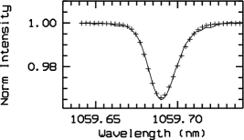
Figure 1: The observed disk-centre Neckel intensity spectrum (solid line) is plotted over the fit (crosses) obtained using a grid of synthetic spectra based on the $\mathrm{CO}^{5}\mathrm{BOLD}$ model computed with Linfor3D.

6 Results and discussion

6.1 The solar P abundance

The different sets of $\log gf$ values for the selected P i lines are very close, so that the derived solar A(P) is quite insensitive to this choice. The solar phosphorus abundance varies by 0.05 dex, from the highest value obtained with the data set of Biemont et al. (1994) to the lower one obtained using Biemont & Grevesse (1973), the corrected value of Berzinsh et al. (1997), or the one from Kurucz & Peytremann (1975). A lower value of the solar phosphorus abundance (0.09 dex below the one obtained using the Biemont et al. (1994) oscillator strength) can be obtained using the non-corrected values from Berzinsh et al. (1997).

With the (corrected) $\log gf$ of Berzinsh et al. (1997) we obtain A(P)=$5.443\pm 0.058$ for the flux spectra considering the whole sample of five lines, A(P)=$5.426\pm 0.064$ for the intensity spectra at disk-centre. The line at 1068.1 nm yields an abundance which is 1.6 $\sigma$ below the mean value, while the other four lines are within one $\sigma$. If we remove this line from the computation, the standard deviation drops by a factor of two and we obtain A(P)=$5.467\pm 0.029,\leavevmode\nobreak\ 5.450\pm 0.042$ for flux and intensity spectra, respectively. The differences in the A(P) determination from intensity and flux spectra could be due to NLTE corrections which usually are different in intensity and flux. Unfortunately, there are no NLTE computations available for these lines. Our recommended solar photospheric abundance is A(P)=$5.458\pm 0.036$, very close to all previous 1D determinations, however 0.1 dex higher than the value found by Asplund et al. (2005) using a 3D model.

The result of Asplund et al. (2005) is difficult to interpret since, according to our model, the 3D corrections for the P i lines in the Sun are small. Asplund et al. (2005) do not provide detailed information on the lines used or of their adopted EWs. They adopted the $\log gf$ of Berzinsh et al. (1997), however they do not specify if they used the “corrected” or ab initio values. If they used the ab initio values the difference is easily understood, otherwise we must conclude that the difference is due either to a difference between their 3D simulation and the $\mathrm{CO}^{5}\mathrm{BOLD}$ one, or due to a difference in the adopted EWs. We point out here that our measured EWs are in quite good agreement with both those of Lambert & Warner (1968), Lambert & Luck (1978) and with those of Biemont et al. (1994)

A detailed summary of the solar phosphorus abundances we derived from individual lines, using different model atmospheres, in given in Table 4. Since the considered lines are not truly weak, the 3D corrections are unfortunately sensitive to the adopted micro-turbulence, and hence must be interpreted with care. The 3D corrections due to horizontal temperature fluctuations only, indicated by the 3D-$\left\langle\mathrm{3D}\right\rangle$ difference, are slightly positive throughout. In all lines, the 3D-$\left\langle\mathrm{3D}\right\rangle$ difference for intensity spectra is systematically higher than for flux spectra, by roughly 0.02 dex. This is presumably due to the fact that the intensity spectra originate from somewhat deeper layers where horizontal fluctuations are larger. We note that the phosphorus lines are formed mostly in the range $-0.5<\log_{10}\tau_{\rm ross}<0$, where the horizontal temperature fluctuations increase with increasing optical depth (see Fig. 2).

The 3D-$\left\langle\mathrm{3D}\right\rangle$ difference increases with the excitation potential of the line’s lower level. In fact, the 3D-$\left\langle\mathrm{3D}\right\rangle$ correction is rather small, not exceeding +0.030 dex for $\xi$=1.0  $\mathrm{km\,s^{-1}}$, and +0.045 dex for $\xi$=1.5  $\mathrm{km\,s^{-1}}$, which we consider as an upper limit.

Figure 2: Relative horizontal RMS temperature fluctuations (on surfaces of equal Rosseland optical depth) in the solar $\mathrm{CO}^{5}\mathrm{BOLD}$ model.

The 3D-$\mathrm{1D}_{\mathrm{LHD}}$ corrections are systematically larger than the 3D-$\left\langle\mathrm{3D}\right\rangle$ difference (by +0.01 to 0.02 dex), but of the same order of magnitude. From that we can conclude that the solar $\left\langle\mathrm{3D}\right\rangle$ and $\mathrm{1D}_{\mathrm{LHD}}$ temperature profiles are very similar.

6.2 3D effects on P for other stars.

As shown above, we obtain only mild 3D effects in our solar phosphorus abundance analysis. They are comparable to the standard deviation (as listed in col. (9) of Table 4) for the weak lines, and a factor four larger than the standard deviation for the strongest line, and hence the 3D effects are hardly relevant. However, 3D effects should become stronger for metal-poor stars where the temperature profiles differ more strongly between $\left\langle\mathrm{3D}\right\rangle$ and $\mathrm{1D}_{\mathrm{LHD}}$ models than for solar metallicity models (Asplund, 2005). Very little work has been dedicated to 3D effects on the phosphorus abundance, and none for metal-poor stellar models. To check the behaviour of the 3D abundance corrections, we theoretically investigated for a few available 3D $\mathrm{CO}^{5}\mathrm{BOLD}$ models the phosphorus 3D-$\mathrm{1D}_{\mathrm{LHD}}$ relation in the resulting synthetic flux spectra.

We find, for three metal-poor models (6300/4.5/–2.0; 5900/4.5/–3.0; 6500/4.5/–3.0), that the difference in the mean temperature profile is the only factor which contributes to the 3D correction. In the metal-poor models, as in the solar model, the maximum contribution to the equivalent widths of the P i lines comes from a well defined region close to the continuum forming layers. Even though the optical depth range contributing significantly is somewhat broader in the metal-poor models than in the solar model, the $\left\langle\mathrm{3D}\right\rangle$ and $\mathrm{1D}_{\mathrm{LHD}}$ models are usually rather close in temperature in this region, and so the effects of the different mean temperature structure are not very pronounced for the considered P i lines. The 3D correction related to the difference in the mean temperature structure of the 3D and $\mathrm{1D}_{\mathrm{LHD}}$ model amounts to $\approx$ +0.05 dex for the –2.0 metallicity model, and to $\approx$ +0.1 dex for the most metal-poor model.

For a 3D $\mathrm{CO}^{5}\mathrm{BOLD}$ model of Procyon (6500/4.0/0.0) the difference in the temperature profile of the $\left\langle\mathrm{3D}\right\rangle$ and $\mathrm{1D}_{\mathrm{LHD}}$ model contributes to more than half of the total 3D correction. In Procyon, P i lines are formed at shallower optical depths than in the Sun by about $\Delta\log\tau\approx 0.3$. In this range the $\mathrm{1D}_{\mathrm{LHD}}$ model is cooler than the 3D $\mathrm{CO}^{5}\mathrm{BOLD}$ one. The related abundance correction depends on the excitation potential (strength) of the line, and for the strongest line it is still less than +0.030 dex. The contribution to the 3D correction related to the horizontal temperature fluctuations ranges from +0.022 to +0.045 dex, increasing with the excitation potential (strength) of the line. In the range where the line is formed, the horizontal RMS temperature fluctuations in Procyon are of the order of 5% to be compared to 1% in the metal-poor models. The total 3D correction is thus less than +0.07 dex for all lines.

7 Conclusions

Using the $\mathrm{CO}^{5}\mathrm{BOLD}$ solar granulation model, we have determined the solar 3D LTE phosphorus abundance to be A(P)=$5.46\pm 0.04$, which compares very well to all previous determinations obtained using 1D models. This can be explained by the fact that the P i lines of Mult. 1 appear to be rather insensitive to granulation effects, at least in the parameter interval explored by us (F and G dwarfs of metallicity from solar to –3.0). These lines can thus be useful to investigate the chemical evolution of phosphorus in the Galactic disk and in moderately metal-poor environments. Below [P/H]=–1.0, however, the lines have EWs smaller than 0.5 pm, becoming exceedingly difficult to observe.

For the P i lines studied in this work, we find small (Sun) to moderate (Procyon, metal-poor stars) 3D abundance corrections. The sign of the corrections is found to be positive in all cases, meaning that the abundances resulting from a 3D analysis are larger than those obtained from a 1D model. Note that this behaviour is consistent with the results obtained by Steffen & Holweger (2002) for S i, which has almost the same ionisation potential as P i (see their Fig. 8). In general, however, the magnitude and sign of the 3D effects depend on the properties of the absorbing ion (ionisation potential, the excitation potential of the lower level, line strength and wavelength), and on the thermodynamic structure of the stellar atmosphere. The results obtained in this work for P i must therefore not be generalised to other elements and other types of stars.

Table 2: Spectroscopic determinations of the solar photospheric phosphorus abundance.

A(P)	$\sigma$	Reference
5.43		Lambert & Warner (1968)
5.45	0.03	Lambert & Luck (1978)
5.45	0.04	Anders & Grevesse (1989)
5.45	0.06	Biemont et al. (1994)
5.49	0.04	Berzinsh et al. (1997)
5.45	0.04	Grevesse & Sauval (1998)
5.36	0.04	Asplund et al. (2005)
5.46	0.04	this work

Table 3: Oscillator strength for the IR phosphorus lines (wavelengths in nm) available in the literature.

$\log gf$					Reference
1051.2	1053.0	1058.2	1059.7	1068.1
–0.21	0.20	0.48	–0.21	–0.10	Kurucz & Peytremann (1975)
–0.23	0.18		–0.24	–0.12	NIST
–0.06	0.31	0.52	–0.14	–0.12	Berzinsh et al. (1997)
–0.13	0.24	0.45	–0.21	–0.19	Berzinsh et al. (1997) corr.
–0.10	0.27	0.49	–0.17	–0.15	Biemont et al. (1994)
–0.24	0.17	0.45	–0.24	–0.13	Biemont & Grevesse (1973)

(NIST: http://physics.nist.gov/PhysRefData/ADS)

Table 4: Solar phosphorus abundances from the various observed spectra, adopting the (corrected) $\log gf$ of Berzinsh et al. (1997).

Spectrum	Wave	EW	A(P) from EW					$\sigma$	3D-$\mathrm{1D}_{\mathrm{LHD}}$		3D-$\left\langle\mathrm{3D}\right\rangle$
	[nm]	[pm]	[dex]	[dex]	[dex]	[dex]	[dex]	[dex]	[dex]	[dex]	[dex]	[dex]
			3D	ATLAS		HM
				1.0	1.5	1.0	1.5		1.0	1.5	1.0	1.5
(1)	(2)	(3)	(4)	(5)	(6)	(7)	(8)	(9)	(10)	(11)	(12)	(13)
KF	1051.2	0.674	5.482	5.476	5.471	5.480	5.475	0.015	0.015	0.019	0.005	0.010
NF	1051.2	0.734	5.523	5.517	5.512	5.521	5.516	0.013	0.015	0.020	0.005	0.010
NI	1051.2	0.811	5.502	5.476	5.473	5.498	5.493	0.012	0.028	0.032	0.022	0.026
DI	1051.2	0.822	5.508	5.483	5.479	5.504	5.500	0.012	0.028	0.032	0.022	0.027
KF	1053.0	1.330	5.431	5.421	5.412	5.427	5.417	0.010	0.019	0.028	0.005	0.015
NF	1053.0	1.340	5.435	5.424	5.416	5.431	5.421	0.010	0.019	0.028	0.005	0.015
NI	1053.0	1.520	5.425	5.392	5.382	5.417	5.408	0.010	0.036	0.044	0.025	0.034
DI	1053.0	1.550	5.436	5.402	5.392	5.427	5.418	0.010	0.036	0.044	0.025	0.034
KF	1058.2	2.280	5.480	5.463	5.448	5.473	5.456	0.012	0.027	0.042	0.006	0.023
NF	1058.2	2.120	5.436	5.421	5.406	5.429	5.414	0.013	0.025	0.039	0.005	0.021
NI	1058.2	2.330	5.407	5.363	5.346	5.393	5.379	0.012	0.047	0.059	0.029	0.043
DI	1058.2	2.330	5.407	5.363	5.346	5.393	5.379	0.012	0.047	0.059	0.029	0.043
KF	1059.7	0.684	5.482	5.475	5.471	5.480	5.475	0.014	0.015	0.019	0.005	0.010
NF	1059.7	0.660	5.464	5.458	5.454	5.462	5.458	0.014	0.015	0.019	0.005	0.010
NI	1059.7	0.748	5.456	5.431	5.427	5.452	5.448	0.012	0.027	0.030	0.022	0.026
DI	1059.7	0.751	5.458	5.433	5.429	5.454	5.450	0.012	0.027	0.031	0.022	0.026
KF	1068.1	0.670	5.370	5.364	5.360	5.368	5.364	0.014	0.015	0.019	0.005	0.010
NF	1068.1	0.617	5.330	5.324	5.320	5.328	5.324	0.015	0.015	0.019	0.006	0.010
NI	1068.1	0.699	5.322	5.297	5.294	5.318	5.314	0.013	0.027	0.030	0.022	0.026
DI	1068.1	0.731	5.343	5.319	5.315	5.340	5.336	0.013	0.027	0.030	0.022	0.026

Col. (1) spectrum identification: DI: Delbouille intensity, NI: Neckel intensity, NF: Neckel flux, KF: Kurucz flux. Col. (2) wavelength of the line. Col. (3) measured equivalent width. Col. (4) phosphorus abundance, A(P), according to the $\mathrm{CO}^{5}\mathrm{BOLD}$ 3D model. Cols. (5)-(8) provide A(P) from 1D models, odd numbered cols. correspond to a micro-turbulence $\xi$ of 1.0 $\mathrm{km\,s^{-1}}$ , even numbered cols. to $\xi=1.5$ $\mathrm{km\,s^{-1}}$ . Col. (9) uncertainty in A(P) due to the uncertainty in the measured EWs. Col. (10)-(13) provide 3D corrections, even numbered cols. for $\xi=1.0$ $\mathrm{km\,s^{-1}}$, and odd numbered cols. for 1.5 $\mathrm{km\,s^{-1}}$, respectively.