A Corona Australis cloud filament seen in NIR scattered light

Abstract

Context. With current near-infrared (NIR) instruments the near-infrared light scattered from interstellar clouds can be mapped over large areas. The surface brightness carries information on the line-of-sight dust column density. Therefore, scattered light could provide an important tool to study mass distribution in quiescent interstellar clouds at a high, even sub-arcsecond resolution.

Aims. We wish to confirm the assumption that light scattering dominates the surface brightness in all NIR bands. Furthermore, we want to show that scattered light can be used for an accurate estimation of dust column densities in clouds with $A_{\rm V}$ in the range 1-15^m.

Methods. We have obtained NIR images of a quiescent filament in the Corona Australis molecular cloud. The observations provide maps of diffuse surface brightness in J, H, and Ks bands. Using the assumption that signal is caused by scattered light we convert surface brightness data into a map of dust column density. The same observations provide colour excesses for a large number of background stars. These data are used to derive an extinction map of the cloud. The two, largely independent tracers of the cloud structure are compared.

Results. In regions below $A_{\rm V}\sim 15^{\rm m}$ both diffuse surface brightness and background stars lead to similar column density estimates. The existing differences can be explained as a result of normal observational errors and bias in the sampling of extinctions provided by the background stars. There is no indication that thermal dust emission would have a significant contribution even in the Ks band. The results show that, below $A_{\rm V}\sim 15^{\rm mag}$, scattered light does provide a reliable way to map cloud structure. Compared with the use of background stars it can also in practice provide a significantly higher spatial resolution.

1 Introduction

Distribution of matter within interstellar clouds can be examined only indirectly by measuring emission or absorption of radiation. Extended maps of interstellar clouds are obtained through (1) emission lines of molecules or atomic tracers, especially CO and HI, (2) thermal emission from dust grains at far–IR and sub-mm wavelengths, (3) optical or near-infrared extinction as traced by star counts, (4) optical or near-infrared reddening seen in the light of background stars, (5) mid-infrared absorption in dark clouds seen against a brighter background, and (6) soft x-ray absorption toward a similarly bright x-ray background.

The correspondence between measured quantities and the actual column densities is not straightforward. Line emission is useful only in a limited range, defined by the chemistry, critical density, and optical depth. The interpretation of measured intensities is further complicated by spatially varying excitation conditions and other radiative transfer effects. Emission from different molecules is often observed to peak at entirely different locations and our view of a cloud’s structure can be seriously biased by the selection of certain tracers. In particular, in cold cloud cores most molecules may have frozen onto dust grains, making them effectively invisible in studies of many molecular lines. At low column densities ($A_{\rm V}\sim$1) the transition between atomic to molecular gas poses similar problems because of the large abundance variations.

Thermal dust emission at far-IR and sub-mm wavelengths provides a complementary tool which, however, is also not free of problems. Conversion into column density requires reliable estimates of the dust temperature and emissivity. Recent studies have shown, that there may be significant variations between clouds and even locally within individual sources (Cambrésy et al. cambresy2001 (2001), del Burgo et al. delburgo2003 (2003), Dupac et al. dupac2003 (2003); Kramer et al. kramer2003 (2003), Stepnik et al. stepnik2003 (2003); Lehtinen et al. Lehtinen2004 (2004), Lehtinen2006 (2006); Ridderstad et al. Ridderstad2006 (2006)). These may be due to grain growth by coagulation and ice mantle deposition (Ossenkopf & Henning ossenkopf1994 (1994), Krugel & Siebenmorgen krugel1994 (1994)) or even physical changes in the grain material itself (e.g., Mennella et al. mennella98 (1998), Boudet et al. Boudet2005 (2005)). Limited sensitivity of observations has restricted most sub-mm emission studies to areas of large column density and/or embedded heating sources. In those cases the spatial temperature and emissivity variations tend to be large, and the density structure can be estimated only indirectly, through complicated modelling.

The problems caused by temperature variations can be avoided by looking at the light attenuation caused by dust particles. Extinction can be traced with star counts (Wolf wolf1923 (1923)) or by examining the change in the colour of stars seen through the cloud. NIR observations have become increasingly important in extinction studies (e.g., Alves, Lada & Lada alves2001 (2001); Cambrésy et al. cambresy2002 (2002)) because, at these wavelengths, extinction properties of grains are believed to be very stable and background stars can still be observed through visually opaque clouds. In the NIR the star count method remains useful beyond $A_{\rm V}\sim$20, provided that deep K-band observations are available. However, at lower extinctions the colour excess method yields better spatial resolution. An independent extinction estimate is obtained for each detected background star, i.e., a very narrow sight line. Errors are usually dominated by the uncertainty of the intrinsic colours that are known only in a statistical sense. An accurate extinction map is obtained only after averaging spatially over many stars. The reliability can be improved by combining results from more than two NIR bands (Lombardi & Alves Lombardi2001 (2001)) and by using adaptive spatial resolution (Cabrésy et al. cambresy2002 (2002)). With dedicated observations a resolution of $\sim$10$\arcsec$ can be reached. In the case of the commonly used 2MASS survey (limiting K_s magnitude $\sim$15) the resolution is, depending on the stellar density towards the examined field, a few arc minutes and the probed range of extinctions is $A_{\rm V}\sim$1–15 mag.

Scattered light provides yet another tracer for studies of interstellar clouds. The first detection of NIR scattered light in a dark nebula illuminated by the normal interstellar radiation field (ISRF) was reported by Lehtinen and Mattila (Lehtinen1996 (1996)). Recently Nakajima et al. (Nakajima2003 (2003)) and Foster & Goodman (Foster2006 (2006)) have demonstrated that with current NIR instruments the scattered radiation can be mapped in moderately optically thick clouds over large areas. In these conditions there should exist a relatively simple relationship between the observed surface brightness and the amount of dust on the line-of-sight. Based on this idea, Padoan, Juvela, & Pelkonen (Padoan2006 (2006)) proposed scattered near-infrared light as a new tracer of cloud column density. As mentioned above, dust properties are relatively constant in the NIR, which also reduces uncertainties related to the scattering properties. In the K-band the optical depth is about one tenth of the visual extinction. Therefore, in regions with $A_{\rm V}$ below 10 mag, the K-band intensity is expected to remain well correlated with dust column density. At higher extinctions the surface brightness starts to saturate. However, Padoan et al. (Padoan2006 (2006)) showed that if the saturation is taken into account, the combination of J-, H-, and K-bands can be used for column density estimation up to $A_{\rm V}\sim 20^{\rm m}$. Juvela et al. (Juvela2006 (2006)) examined further the relationship between surface brightness and column density using a series of inhomogeneous cloud models. They concluded that the errors in the column density estimates remain small even in the presence of expected dust property variations and in the case of anisotropic external illumination. Furthermore, they noted that the comparison of surface brightness and colour excess methods makes it possible to identify and correct effects caused for example by anisotropic illumination. As a column density tracer, scattered light was estimated to be as reliable as the use of background stars. At the same time, scattered light could provide much higher resolution.

In order to examine the use of scattered light as a tracer of interstellar clouds we have carried out deep J-, H-, and Ks-band observations of a filament in the northern part of the Corona Australis cloud. Based on 2MASS data, at the resolution of a couple of arc minutes, the extinction was estimated to be in the range $A_{\rm V}=1-10\,$mag, a range suitable for this method (see Fig. 1). The diffuse surface brightness was detected in all three bands and, therefore, can be used for estimation of column densities over most of the observed area. The imaging provides simultaneously photometry for a large number of background stars so that an extinction map can be constructed based on the colour excesses of those stars. The comparison of surface brightness and extinction values makes it possible to estimate the reliability of scattered light as a probe of cloud column density. We will show that the observed NIR surface brightness is consistent with the assumption that the signal is caused by light scattering. In particular, we will show that below $A_{\rm V}=15^{\rm m}$ the column density estimates from surface brightness data and from background stars are consistent with each other.

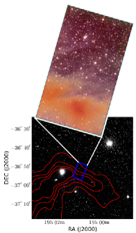
Figure 1: The lower frame shows a Digitized sky survey image of the northern part of the Corona Australis Molecular cloud. The contours indicate optical extinction determined with the NICER method using stars from the 2MASS survey. The contours are drawn between 2 and 10 magnitudes at steps of two magnitudes. The box shows the outlines of the area observed in the near-infrared with the SOFI instrument. The bright region east of the mapped area is a reflection nebula associated with the young star R Corona Australis. The upper frame shows an image composed of our the J, H, and Ks band observations. The intensity scale has been adjusted to bring out faint surface brightness. High J/Ks ratios corresponds to blue, and low ratios to red colour.

We present in Sect. 2 the observations and in Sect. 3 a qualitative analysis of the surface brightness data. In Sect. 4 the surface brightness measurements are converted into a map of column density using the method outlined by Padoan et al. (Padoan2006 (2006)). In Sect. 5 the reddening of the light from background stars is analyzed using the NICER method, resulting in another, largely independent map of column density. The results are compared with each other in Sect. 6. The discussion of the results is presented in Sect. 7 and summarized in Sect. 8.

In this paper we limit the study to regions with $A_{\rm V}$ below $\sim$15^m where conversion between surface brightness and column density is more straightforward. In a forthcoming paper we will carry out three-dimensional radiative transfer modelling of the whole field. This will enable us to estimate or derive lower limits for column densities also in the most optically thick regions. In that paper we will extend comparison with the NICER method beyond $A_{\rm V}=20^{\rm m}$, and look for signs of dust property variations within the filament.

2 Observations

The field was observed with the explicit purpose of testing the conversion between scattered light and column density. From the Corona Australis molecular cloud we selected a region where the visual extinction was estimated to be in the range $A_{\rm V}=1-10$ magnitudes, and where there were no strong infrared sources within the field, either physically within the cloud or seen in projection. The field is centered at $19^{\rm h}0^{\rm m}51^{\rm s}$, $-36\degr 52\arcmin 30\arcsec$ (J2000) and covers part of the filament that extends SW from the northern end of the Corona Australis cloud. In equatorial coordinates the filament runs horizontally across the southern end of the image (see Fig. 1). In the northern end the image extends outside the filament to a region of low extinction. The extinction was originally estimated using 2MASS data and the NICER method. At the resolution of 3 arc minutes the range of visual extinctions was $A_{\rm V}=1-10$ magnitudes (see Fig. 1), although it was also clear that higher spatial resolution could reveal smaller areas with much higher extinction. For the filament itself the extinction decreases towards west, where the 2MASS extinction drops rapidly below 5 magnitudes. The area has been mapped in 1.2 mm continuum by Chini et al. (Chini2003 (2003)). In those observations the filament is not smooth but appears to have several distinct density enhancements. This is already confirmed by Fig. 1. Within the field imaged in NIR the brightest star has a Ks band magnitude of 12.1.

The observations were made in August 2006 using the SOFI instrument on the NTT telescope. The observations were carried out as ON-OFF measurements so that the faint surface brightness could be recovered. We used two ON-fields that overlap each other by $\sim 1\arcmin$. Four OFF fields were selected based on IRAS images and 2MASS extinction maps from regions with low dust column density. The observations of the ON- and OFF-fields were interleaved in a sequence of ON-2 – OFF – ON-1 in order to minimize the effect of sky variations. The OFF-field was varied in different observation blocks in order to average out any faint background gradients that might still exist in the OFF-fields. Each observed frame was an average of six 10 second exposures, corresponding to an integration time of 1 minute. After each sequence, the telescope returned to ON-2. At this point random jitter was added in order to avoid holes caused by bad pixels. The total integration times for each ON-field was 65 minutes in J, 91 minutes in H, and 260 minutes in Ks band (see Table 1).

Table 1: Positions and total integration times of the observed ON and OFF fields. The last column gives list for the OFF fields the extinction estimates of Schlegel, Finkbeiner & Davis (SFD (1998)).

Field	centre position	$t$(J)	$t$(H)	$t$(Ks)	$A_{\rm V}$
	(J2000)	(min)	(min)	(min)	(mag)
ON-1	$19^{\rm h}0^{\rm m}54^{\rm s}$, $-36\degr 54\arcmin 0\arcsec$	65	91	260	–
ON-2	$19^{\rm h}0^{\rm m}48^{\rm s}$, $-36\degr 51\arcmin 0\arcsec$	65	91	260	–
OFF-1	$18^{\rm h}58^{\rm m}14^{\rm s}$, $-36\degr 50\arcmin 11\arcsec$	18	26	78	0.45
OFF-2	$18^{\rm h}58^{\rm m}15^{\rm s}$, $-36\degr 34\arcmin 43\arcsec$	18	26	89	0.35
OFF-3	$18^{\rm h}56^{\rm m}59^{\rm s}$, $-36\degr 53\arcmin 5\arcsec$	18	26	80	0.33
OFF-4	$18^{\rm h}57^{\rm m}34^{\rm s}$, $-36\degr 50\arcmin 11\arcsec$	11	13	13	0.33

The observations were calibrated to 2MASS scale by using photometry of ten selected stars in each individual frame. Their average was used to correct the observed fluxes to above the atmosphere. After calibration the two ON-fields were mosaiced together using the overlapping area. This required an addition small correction to ON-1, to have the same number of counts in the overlapping area as ON-2. Finally, a correction was added to the combined frame to place the minimum of the diffuse emission at zero. After removing borders with high noise, the remaining imaged area is 8.4$\arcmin\times$5.0$\arcmin$. For studies of the surface brightness we produced another set of images where we try to eliminate the effect of stars. Stars were first removed using DAOPHOT task ALLSTAR. In many cases this left noticeable residuals at the location of bright stars. These were removed by interpolating over the masked stellar image. This affects only the figures because in the analysis these pixels were still kept masked. The effect of some bright stars extends beyond the area masked by DAOPHOT. In these cases the masks were extended manually, removing areas were the surface brightness enhancement was visibly above the general background. Finally, faint stars that were not identified by DAOPHOT were removed with median filtering. The filter size was 14 pixels or 4.0 arc seconds which is roughly equal to 4 times the FWHM of the point spread function. The final J-, H-, and Ks-band surface brightness images are shown in Fig. 2. This and the subsequent images are rotated so that equatorial north is towards lower left. In this orientation the surface brightness increases to the right and the filament runs vertically through the right hand side of the images. The Ks-band can be assumed to correlate best with the column density. In J- and H-bands the optical depths are higher, the surface brightness saturates earlier and finally decreases so that the most opaque regions correspond to local minima. There is a small local minimum also in Ks, at the location of presumably the highest column density. On other sightlines, where at least Ks surface brightness is not yet completely saturated, the scattered light should be unequivocally correlated to the column density.

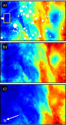
Figure 2: Observed surface brightness in J, H, and Ks bands (frames a, b, and c, respectively). Bright stars identified by DAOPHOT were removed and replaced with interpolated surface brightness. Faint stars have been eliminated with median filtering. In the J-band image (frame $a$) the white regions correspond to areas around bright stars that were masked and removed from subsequent analysis. The box denotes an area used as a reference point for the NIR surface brightness. In frame $c$ the arrow shows the direction of equatorial north.

3 Correlations between NIR surface brightness maps

In this section we examine the relations between the three near-infrared bands. Figure 3 shows the J- and H-band surface brightness plotted against the Ks-band surface brightness. The data of Fig. 2 was convolved to a resolution of 10 arc seconds using a gaussian beam, while the plotted values correspond to a sampling of 5 arc seconds. The zero point of the surface brightness values is set using the reference area marked in Fig. 2.

Figure 3 is qualitatively consistent with the idea that the surface brightness is caused by light scattering. The relations have a linear part and at higher Ks-band intensities (higher column densities) saturation starts first at the shorter wavelengths. For the J-band this happens below $I_{\rm Ks}=0.2$ MJy/sr, whereas for the H-band the change is more gradual and complete saturation is reached only after $I_{\rm Ks}=0.3$ MJy/sr. The expected optical depth in the J-band is about 1.7 times the value in the H-band, so that the difference between the J- and H-bands is of the expected magnitude. Although the dispersion increases towards higher column densities, i.e. towards the centre of the filament, the NIR intensities do still follow a relatively tight relation. Around $I_{\rm Ks}=0.5$ MJy/sr both J and H intensities show a hook, when the correlation with the Ks-band becomes negative. Again, this is the expected behaviour for scattering in optically thick clouds. Maximum surface brightness is reached when, for the wavelength in question, the optical depth is around 1-1.5. Because H-band does suffer complete saturation one can already estimate that, assuming a normal extinction curve with $A_{\rm V}/A_{\rm H}\sim$6, the visual extinction must exceed 10^m in a large part of the filament.

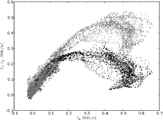
Figure 3: The observed J band intensities (black dots) and H band intensities (grey dots) plotted against the Ks-band surface brightness. The data have been convolved to a resolution of 10 arc seconds and sampled at intervals of FWHM/2.

If the surface brightness is to be used for column density estimation, there must exist a single (although not necessarily linear) relationship between column density and surface brightness. Therefore, we examine next the dispersion around the mean relation. In Fig. 4 we show again the relation between the J and Ks bands. This time we plot with different symbols groups of measurements that deviate most from the mean behaviour. In the second frame the distribution of these measurements is overlaid on the J-band image.

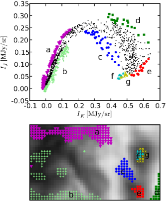
Figure 4: Upper frame: J-band intensity plotted against the Ks-band intensity. Some groups of measurements that deviate from the general trend are marked with different symbols. Lower frame: Map of the Ks-band intensity. The groups of observations identified in the upper frame are marked here with the same symbols. All data have been smoothed to a resolution of 10$\arcsec$.

The linear part of the relation ($I_{\rm Ks}<0.15$MJy/sr) corresponds to optically thin regions ($A_{\rm J}\la 1^{\rm m}$). Deviations from the average relations could be caused by local changes in dust properties or variations in the intensity or spectrum of the illuminating radiation. However, when optical depths are low the radiation sources should be very close before they can produce significant intensity gradients.

Figure 4 shows that within the linear part high J/Ks ratios are found to be systematically higher on the upper border (region $a$) and lower on the lower border (region $b$) as compared to the average. In between there are a few separate areas belonging to region $b$, but these can be attributed to uncertainty in background subtraction (the region that was used to define the zero level, see Fig. 2) and remaining artifacts around bright stars. The regions $a$ and $b$ can also be identified in H/Ks images but are not visible in the J/H ratio (see Appendix A). Therefore, the features must originate in the Ks-band image. Moving upwards, the ratios J/Ks and H/Ks first increase at the lower border, remain almost constant for a while, until in region $a$ they increase again rapidly before a final drop at the upper border. Even excluding borders affected by increased noise levels, the change cannot be described as a smooth gradient across the image. One could interpret, for example, region $a$ as a result of measurement and reduction errors, e.g. imperfect flat fielding. However, the changes do partly coincide with definite cloud structures. The dark area on the left of region $c$ and above the rightmost tip of region $b$ is visible in J/H and H/Ks images as a region of lower Ks-band emission.

Above $I_{\rm Ks}\sim 0.2$ MJy/sr saturation causes a turnover in the relation between J and Ks intensities. The ratio of J and Ks optical depths should be $\sim$2.5. Therefore, the relation between Ks intensity and column density should still remain linear in these regions. Figure 4 shows one distinct group of points for which the J intensity is abnormally low. According to Fig. 4b this can be identified as a wedge of low column density that runs into the filament (region $c$). One possible explanation suggested by the geometry is that the shadowing provided by the filament on both sides of the wedge has weakened the local radiation field, the effect being strongest in the J-band.

The situation is reversed in the lower right hand corner of the field (Fig. 4, region $d$) which exhibits stronger than average J band intensity. Based on the Ks band surface brightness the column density should be similar as in region $c$. However, for a given Ks-band intensity the value in the J-band can be higher by a factor up to three. Note that for most of the cloud the points do follow a well-defined relation which falls between the extremes represented by regions $c$ and $d$. Region $d$ is on the other side of the optically thick filament where the spectrum of the ISRF could be different. The average grain size could also be smaller if, in that region, a shock wave has destroyed larger grains. On the other hand, region $d$ is at the corner of the field and one cannot completely rule out the possibility that it is merely an artifact.

As one moves to the left of region $d$, one enters the main filament and region $e$, which coincides with a local minimum in the J intensity. Over this short distance the Ks-band intensity remains roughly constant while in J the intensity is reduced by a factor of $\sim$3–4. The minimum seen in Fig. 2a suggests that this is a local maximum of column density and, while region $d$ is clearly outside the densest filament, region $e$ represents the centre of it. However, according to Fig. 2 in Ks-band the intensity peaks just SW of this position. This could mean that within $e$ also the Ks band is saturated and, therefore, locally anticorrelated with column density. This would be consistent with the observation that the Ks-band intensity is still practically the same as in region $d$, that is, in a region with seemingly much lower column density. Assuming that the Ks-band has reached complete saturation, one can estimate the optical depth to be above $\tau_{\rm Ks}\approx$1.5, or correspondingly the visual extinction to be above $A_{\rm V}\approx$15^m. Another explanation would be that the Ks-band still follows the column density distribution, but anisotropic illumination has shifted the J-band minimum towards the upper left. In other words, the filament would be illuminated more strongly from the lower right direction.

The final two regions, $f$ and $g$, correspond to the most opaque region because in Fig. 2a the local minimum is seen at all three wavelengths. Furthermore, in Fig. 4 these form the end point in the non-linear relation between J and Ks intensities. By dividing this tip into two parts we can see that even here points fall systematically into separate locations. Region $g$ represents points that are relatively brighter in Ks than in J. In the map (Fig. 4b) these form a crescent on the right hand side (south) of the column density peak. Correspondingly on the left side (north) the ratio J/Ks is larger. This suggests that the filament is illuminated more strongly from the left. As one moves to the right, the intensity of the illuminating radiation would become weaker and redder and, for a given column density, the scattered radiation would not only be weaker but would also exhibit a lower J/Ks ratio. The systematic shift in the location of the intensity minimum was already visible in Fig. 2.

The regions c–g can also be identified both from relations between H and Ks bands and from the relation between J and H bands. This means that it is unlikely that any of these features could have been produced by measurement errors. On the other hand, the regions a and b are probably largely artifacts. They may be indicative of the level of systematic measurement errors that could be expected in observations of faint surface brightness. These would ultimately set the limit to the accuracy at which column densities can be determined based on surface brightness measurements.

4 Column densities based on scattered light

Padoan et al. (Padoan2006 (2006)) presented formulas for converting scattered surface brightness into dust column density. At low visual extinctions the relationship is linear and column densities could be mapped using observations at any single wavelength. However, in order to obtain absolute values, some assumptions must be made about the illuminating radiation field and the dust properties. When the visual extinction reaches $A_{\rm V}\sim 10^{\rm m}$, even NIR surface brightness values start to saturate. The effect begins at shorter wavelengths and the relationship with column density becomes increasingly more non-linear as the column density increases. In inhomogeneous clouds with line-of-sight extinction $A_{\rm V}=10^{\rm m}$ the non-linearity was found to be only $\sim$20%. Padoan et al. (Padoan2006 (2006)) and Juvela et al. (Juvela2006 (2006)) also discussed column density estimation using combined measurements in J-, H-, and Ks-bands. In diffuse regions the intensity ratios are determined by the spectrum of the external radiation field and by the dust scattering properties. In more opaque areas the intensity ratios also depend on the degree of saturation. In other words, the intensity ratios carry independent information on the line-of-sight column densities.

Following Padoan et al. (Padoan2006 (2006)) we first approximate the relationship between surface brightness $I_{\lambda}$ and visual extinction $A_{\rm V}$ with the equation

$$I_{\lambda}=a_{\lambda}\times(1-e^{-b_{\lambda}A_{\rm V}}).$$ (1)

Based on numerical simulations this functional form is approximately correct as long as saturation remains weak. On the other hand, the equation cannot describe strong saturation and the associated turnover in the relation between intensity and column density. In the present case, this form remains applicable outside the filament but it cannot be used to describe the J- and H-band observations towards the centre of the filament. If J-, and H-bands are compared with Ks-band data, $A_{\rm V}$ can be eliminated

$$I_{\lambda}=a_{\lambda}\times(1-(1-I_{\rm K}/a_{\rm K})^{b_{\lambda}/b_{\rm K}}).$$ (2)

The parameters $b_{\lambda}$ depend mainly on NIR dust properties and their ratios can be assumed to be known. The parameters $a_{\lambda}$ can, in principle, be obtained by fitting the Eq. 1 to observations. Once the parameters have been obtained, extinction estimates are derived from the equation

$$A_{\rm V}=-\left[log(1-I_{\lambda}/a_{\lambda})\right]/b_{\lambda}.$$ (3)

The final value of the column density can be calculated as a weighted sum of estimates derived for J-, H-, and Ks-bands.

In practice we fit to observations a parametric curve defined by Eq. 1. The minimum distance between each observed triplet ($I_{J}$,$I_{H}$,$I_{Ks}$) and the curve is found by minimization. The sum over squared distances gives an estimate of the goodness of fit, the minimization of which gives values for the parameters $a$ and $b$. The parameter $b_{\rm Ks}$ is kept constant, because, as seen in Eq. 2, observations can be used to fix only the ratio of the $b$-parameters. In the fit the absolute value of $b_{\rm Ks}$ is unimportant, but it will determine the final transformation into column density units. We use for $b_{\rm Ks}$ a value of 0.125 mag^-1 obtained from simulations made by Juvela et al. (Juvela2006 (2006)). Those calculations were based on dust properties given in Draine (Draine2003a (2003)) and data files which are available on the web . The assumed ratio of total to selective extinction is $R_{\rm V}=A_{\rm V}/E(B-V)=3.1$. The default extinction curve would predict $b_{\rm Ks}\sim$0.1 mag^-1, but, as discussed in Juvela et al. (Juvela2006 (2006)), $b$ cannot be interpreted as a pure extinction cross section.

Figure 5 shows the observed J- and H-band intensities values plotted against the Ks-band intensities. The saturated part of the relations ($I_{\rm Ks}>0.4$ MJy/sr) is not shown. Here we avoid image borders, using only data between declinations -36$\degr$52^m30^s and -36$\degr$50^m0^s. We also remove the remaining pixels belonging to region $b$ (see Fig. 4). The resolution is still 10$\arcsec$. In the $H$-band one can see that not all regions follow exactly the same relation, and there is a separate population with low $H/Ks$ ratios. At high $I_{\rm Ks}$ these are close to the already masked region $c$, and at lower $I_{\rm Ks}$ the points are associated with emission close to the region $b$. In Fig. 5 we also show the fitted analytic curve, projected into ($I_{\rm Ks},I_{\rm J}$) and ($I_{\rm Ks},I_{\rm H}$) planes. The fit is done using points with $I_{\rm Ks}<0.4$ MJy/sr. The limit corresponds to more than 20^m in visual extinction.

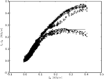
Figure 5: The surface brightness in the J-band (dots) and H-band (crosses) plotted against the Ks-band intensities. The lines show the fitted relations (see text).

For each observed point (J,H,Ks) the column density can now be estimated by locating the nearest position on the curve, and using Eq. 3. The selected value of $b_{\rm Ks}$ defines the final column density scale. The effect of saturation decreases the correlation between intensity and column density near the filament, especially in the $J$ band. On the other hand, at low column densities the relative noise is largest in the Ks band. Therefore, we adjust the relative weighting of the bands when estimating the minimum distance from the curve. At low column densities the relative weights are $J:H:Ks=1:0.8:0.2$, and they change linearly so that at the highest column densities the weights are 0.2:0.8:1.6.

There is one additional complication that arises from the fact that the reference area marked in Fig. 2a is not free from extinction. We could use Eq. 1 and the surface brightness values relative to the reference area and this way obtain estimates for extinction relative to the reference area. However, a wrong zero point of the $A_{\rm V}$ axis could cause a small bias because the relation between surface brightness and column density is non-linear. The zero point is not important for Eq. 1 itself because that is only an analytic fit to observed data. However, we will use a value of $b_{\rm K}$ that is based on simulations where zero intensity does correspond to zero extinction. At low column densities, the intensity is proportional to $a_{\rm K}\times b_{\rm K}$. An inaccurate value of $b_{\rm K}$ is compensated by $a_{\rm K}$ that is obtained from a fit to observations. The bias would exist mainly at high column densities. When one ignores extinction in the reference region, the expected saturation of surface brightness and the estimated column density will both be underestimated. Based on 2MASS data and the NICER method (Lombdardi & Alves Lombardi2001 (2001)) the minimum extinction in our field is $A_{\rm V}\sim 1.5^{\rm m}$. In the next Section we use our NTT observations and the NICER method to obtain a more accurate value, which is 1.8^m for the reference area. We use this information already now, replacing Eq. 1 with a corresponding equation that takes into account the fact that zero intensity (relative to the reference area) corresponds to an extinction $A_{\rm V}=A_{\rm ref}$,

$$I_{\lambda}(A_{\rm V})-I_{\lambda}(A_{\rm ref})=a_{\lambda}\times(e^{b_{\lambda}A_{\rm ref}}-e^{b_{\lambda}A_{\rm V}}).$$ (4)

Another possibility would be to obtain the zero point for surface brightness scale from OFF fields. However, the atmospheric emission and its variations make it difficult to compare surface brightness levels between separate fields. The magnitudes of the background stars are less affected by a changing background level and provide a more reliable, albeit an indirect way to fix the zero point of the extinction scale.

Figure. 6 shows a map of the estimated column densities, here in units of visual extinction (as defined by the selected value of $b_{\rm Ks}$). Column densities have been calculated for all pixels, including, for example, also regions $a$ and $b$ (see above). The resolution is 10$\arcsec$. When data below $I_{\rm Ks}=0.4$ MJy/sr was fitted, we obtained for $a_{\rm Ks}$ a value of 0.50 MJy/sr. This is at the same time the surface brightness that the analytical formulas predict for infinite column density. The map does contain pixels where intensities are larger than the value of the parameter $a$ and for which, therefore, no column density can be estimated using this method. This is caused partly by observational noise and partly because the analytic fit was done using only data from areas with lower $A_{\rm V}$. In the plot the $A_{\rm V}$ scale is cut at $15^{\rm m}$. Above this limit the saturation becomes so strong that predictions of $A_{\rm V}$ become unreliable. Equation 1 can clearly describe the surface brightness only up to the point of turnover, and close to those values the measurement errors are strongly amplified. At high $A_{\rm V}$ the results may also be biased, because the formulas do not take into account shadowing caused by the optically thick filament. Because of attenuation of the intensity of the local radiation field the observed surface brightness decreases and, as a result, the column density is underestimated. In more diffuse areas, e.g. in regions $a$-$c$, the results can be affected by the deviating colours that were discussed above.

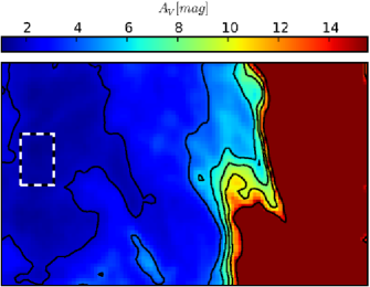
Figure 6: A map of column densities estimated based on the observed scattered surface brightness and Eq. 3. The contours are drawn at $A_{\rm V}$ equal to 2, 4, 6, 8, 10, and 15 magnitudes. The resolution of the map is 10$\arcsec$ and the pixel size is 5$\arcsec$. For the reference area marked with the box the extinction was assumed to be $1.8^{\rm m}$ (see text). No estimates are shown above $A_{\rm V}=15^{\rm m}$ because Eq. 3 becomes unreliable at high extinctions.

5 Extinction map from background stars

We use observations of the background stars and the NICER algorithm (Lombdardi & Alves Lombardi2001 (2001)) to derive an extinction map for the observed field. NIR images give colours for a large number of stars that reside behind the Corona Australis cloud and whose radiation suffers reddening because of the dust in the cloud. Visual extinction can be estimated by comparing these reddened colours with the colours observed towards an unextincted off–region. The method relies on the assumption that, in a statistical sense, the intrinsic colours of the stars are similar in the off–region and in the region studied. Knowledge of the dust extinction curve is needed in order to combine the information of several bands and in order to transform colour excesses into values of visual extinction, $A_{\rm V}$.

In the following we assume a normal extinction curve (Cardelli et al. Cardelli89 (1989)). Analysis of 2MASS data that employed a dark off-region well outside the cloud suggested that there is significant extinction everywhere in our ON fields. Therefore, in order to obtain an absolute zero point for the $A_{\rm V}$ scale we use the field OFF-1 as the reference region. In the ON fields, even with our deep NIR observations, the stellar density is too low to be able to determine the extinction at a resolution of $10\arcsec$. The number of stars for which magnitudes could be measured in all three bands is less than 1000 for the whole map, and the stellar density decreases rapidly as one moves into the optically thick filament. Therefore, in Fig. 7 we show an extinction map calculated at a resolution of 20$\arcsec$. The sigma clipping was done at a 3-$\sigma$ level (see Lombdardi & Alves Lombardi2001 (2001)). The stars used for the extinction measurement are plotted in the same figure. Note that although the extinction map does contain a region with predicted extinction $A_{\rm V}>20$, that region contains very few stars. For the reference area (see Fig. 2a) used in surface brightness plots we obtain an average extinction of $A_{\rm V}=1.8^{\rm m}$. This takes into account the estimated extinction within the OFF fields (see Table 1). This value was already used in the previous Section, in the conversion between surface brightness and $A_{\rm V}$.

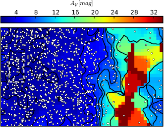
Figure 7: Extinction map estimated based on the reddening of background stars. The contours are drawn at levels of 2, 4, 6, 8, 10, and 15 magnitudes of $A_{\rm V}$. The resolution is $20\arcsec$ and the pixel size is 10$\arcsec$. The stars used in the calculation are marked as dots. The average extinction within the marked reference area is $A_{\rm V}=1.8^{\rm m}$.

6 Comparison of column density estimates

In this section we compare in more detail the column density estimates obtained from scattered light with those derived from background stars. We limit the comparison to areas where the scattered light predicts values $A_{\rm V}<15^{\rm m}$. The limit is set because the methods of Sect. 4 are no longer applicable when Ks band surface brightness suffers significant saturation. In this Section we examine only column density estimates north of the filament (left of the filament in the orientation used, for example, in Fig. 2). In Sect. 4 the parameters were determined using only that area. On the other side of the optically thick filament the radiation field could be different, and we return to this question later in Sect. 7.

6.1 Comparison of extinctions

Some conclusions can be drawn already by looking at Figs. 6 and 7. The maps agree in their main features and give even quantitatively similar $A_{\rm V}$ estimates. In spite of the fact that Fig. 6 has twice the resolution of the NICER map it is significantly smoother. This strongly suggests that even at the resolution of $20\arcsec$ the NICER map still contains significant noise caused by the scatter in the intrinsic colours of the background stars. In many places where the details of the two $A_{\rm V}$ maps differ, the differences can be attributed to low stellar density. For example, in the lower central part of Fig. 6, the surface brightness data reveal an elongated region with dimensions of $\sim 90\arcsec\times 30\arcsec$ that in this figure is surrounded by a contour at $A_{\rm V}=4^{\rm m}$. The feature should be resolved at 20$\arcsec$ resolution, but the NICER map contains only a hint of this feature because there happens to be no background stars within this area. The wedge of low extinction that extends into the filament is much narrower in the map that is based on surface brightness data. This is not caused by the difference in the selected resolution but rather by the fact that also this area contains only a few background stars. The surface brightness data also predict a sharp increase of extinction close to the filament. This is probably real although a gradient could be altered if the parameters used in the analysis were wrong. For example, if parameter $b_{\rm K}$ were overestimated, one would expect high surface brightness values to be strongly saturated and the higher the intensity the more would the column density be overestimated. The presence of such errors cannot be confirmed or refuted by the NICER data. There the 15^m contour is certainly further away from the lower contours but stellar density is again too low for this to be significant. The NICER map was created using all stars where we had photometric values for all three bands. The outcome is not improved when the map is made using all stars detected in two or three bands. The number of stars is naturally increased but at the same time the errors for individual stars increase.

In the following the comparison is carried out at the resolution of 20$\arcsec$, because of the lower resolution of the colour excess maps. Figure 8 shows the resulting correlation between the column density estimates based on scattered light, $A_{\rm V}^{\rm sca}$, and those derived using the NICER method, $A_{\rm V}^{NICER}$. The plot is limited to the region with $A_{\rm V}<20^{\rm m}$ and, therefore, includes the regions $a$–$c$ discussed in Sect. 3. The pixels belonging to the areas $a$ and $b$ do not deviate from the general relation. In the range $A_{\rm V}^{NICER}=8-11^{\rm m}$ most of the points above the average relation correspond to the region $c$. In the plot the two $A_{\rm V}$ scales are related, but only indirectly. For NICER the absolute scale is defined by the assumed extinction law (Cardelli et al. Cardelli89 (1989)). For scattered light the scaling depends on the selected value of $b_{\rm Ks}$. This was obtained from simulations that assumed a dust model consistent with a similar extinction law (Draine Draine2003a (2003)). However, while the NICER estimates depend only on total dust extinction cross sections, the observed intensity of scattered light also depends on the scattering function and albedo of dust grains. In Fig. 8 the extinction estimates are consistent with each other, and, in first approximation, $A_{\rm V}^{\rm sca}\sim A_{\rm V}^{NICER}$ (dashed line in Fig. 8). This can be taken as further confirmation that most of the observed surface brightness is indeed caused by scattering from dust particles, because the values of $A_{\rm V}^{\rm sca}$ do explicitly depend on this assumption and the ratio between extinctions in the $Ks$ and $V$ bands. The ratios between constants $b$ and the values of the constants $a$ at J, H, and Ks were obtained directly from the data. Therefore, we did not need to assume any particular intensity or spectral shape for the illuminating radiation. The only assumption is that these remain constant over the mapped area.

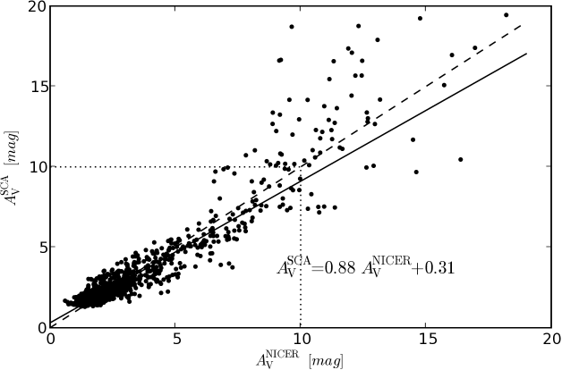
Figure 8: Correlation between the extinction derived using the NICER method, $A_{\rm V}^{\rm NICER}$, and the values derived from surface brightness measurements, $A_{\rm V}^{\rm SCA}$. The comparison is limited to area left of the filament (see Fig. 6), where the surface brightness method predicted extinctions below 20^m. The points correspond to pixels in Fig. 7: the resolution is 20$\arcsec$ and the sampling is done at intervals of 10^″.

At low $A_{\rm V}$ the scatter increases because of measurement errors. The extinction maps of Figs. 6 and 7 already indicated that the scatter would be dominated by uncertainty in the NICER method. In the colour excess method the uncertainty has two components, one arising from photometric measurement errors and another from the scatter in the intrinsic colours of background stars. For a more thorough discussion of the statistical basics of the colour excess method see Lombardi (Lombardi2005 (2005)). That paper also describes the combination of the colour excess and star count methods first discussed by Cambrésy et al. (cambresy2002 (2002)). In our case the formal errors are dominated by variation in the intrinsic colours. However, the error estimates reported by the NICER program do not take into account true opacity variations within the beam that is used for spatial averaging of the extinction values of individual stars. If it is estimated based on this dispersion, the error increases with increasing extinction. At high $A_{\rm V}$ there can also be a significant bias because background stars are observed preferentially from those parts of the cell where extinction is lower. In Fig. 8, at high extinctions, the surface brightness data tend to predict larger $A_{\rm V}$ values than what the background stars do. This can be a direct result of the low number of stars seen through the filament. In the NICER maps and especially in the region $A_{\rm V}\sim 10-15^{\rm m}$ many values are obtained by interpolating over very long spatial distances. In the case of the filament, this can result in significantly underestimated extinction values. The scatter in the $A_{\rm V}^{\rm NICER}$ values carries information on column density variations within the cells that are used in the calculation of the extinction map (Padoan et al. Padoan1997 (1997); Juvela Juvela1998 (1998); Lada et al. Lada1999 (1999)). However, in our case those variations are dominated by the large scale gradients associated with the filament rather than any small scale inhomogeneities.

6.2 Comparison of errors

In Fig. 9 we plot two error estimates for the NICER method calculated for $20\times 20\arcsec$ cells. The first error estimate is obtained by combining the effects of photometric errors, $\sigma_{\rm obs}$, and the scatter in the intrinsic colours of the stars, $\sigma_{\rm intr}$. The error in $A_{\rm V}$ values was estimated by determining the variation in extinction maps, when noise was added to the input data. For the errors of input magnitudes we use the DAOPHOT error estimates. The scatter of intrinsic colours was estimated from an OFF field and this dominates the overall uncertainty. For individual stars the estimated error is $\sigma(A_{\rm V})\sim 1.5^{\rm m}$ almost irrespective of the extinction. At low $A_{\rm V}$ the 20$\times 20\arcsec$ cells contain typically $\sim$10 stars.

The second error estimate is obtained by calculating the scatter of the observed $A_{\rm V}$ values of individual stars in a cell and by dividing this number with the square root of the number of stars. For a flat $A_{\rm V}$ map the two error estimates should be equal provided that the errors $\sigma_{\rm obs}$ and $\sigma_{\rm intr}$ are correctly determined. However, the second error estimate also includes some information on the column density variations within the map cells. If there are strong extinction gradients it could overestimate the true error. On the other hand, it does not take into account the bias that exists because of the anticorrelation between the column density and the surface density of the observed background stars. Figure. 9 shows that the error estimates obtained with the second method increase more rapidly as extinction increases. This is probably caused by the steep extinction gradients. The plot extends only up to $A_{\rm V}\sim 12^{\rm m}$ because, at higher extinctions, there are very few cells with more than one star per cell.

In the case of scattered light the estimation of the uncertainty of the surface brightness measurements is not quite straightforward because the images also contain true surface brightness variations at all scales and we do not know how the errors are correlated over different distances. In order to remove real large scale structures, we filtered out all Fourier terms corresponding to spatial frequencies $k<0.1$ arcsec^-1. One could estimate the uncertainty of surface brightness by calculating the remaining standard deviation between individual pixels. However, if the noise is correlated over several pixels, this will underestimate the true errors. Instead, we divided each 20$\arcsec\times 20\arcsec$ cell into $4\times 4$ sub-regions and used their dispersion to estimate the error of the mean. The results (circles in Fig. 9) should be independent of correlated errors at scales below 5 $\arcsec$. The estimates still include the effect of true column density variations at this scale and, therefore, could overestimate the true uncertainty.

The Fig. 9 indicates that, in our case, the uncertainty in $A_{\rm V}$ is smaller for the surface brightness method than for the colour excess method. The previous analysis does not fully take into account the bias of the estimates. Nevertheless, the results suggest that the sampling errors caused by the limited number of background stars have a significant contribution to the scatter seen in Fig. 8, especially at high extinctions. Lombardi (Lombardi2005 (2005)) described a maximum likelihood method that, in the presence of foreground stars, showed smaller bias than the NICER method. The use of such schemes might improve the results of the colour excess method also here but, of course, cannot overcome the basic problem of an insufficient surface density of the background stars.

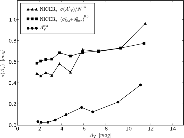
Figure 9: Estimated uncertainty of extinction estimates as a function of $A_{\rm V}$. For the surface brightness method the dispersion in estimates of $A_{\rm V}$ is shown as solid circles. For NICER the dispersion of intrinsic colours was estimated from the field OFF–1. Adding photometric errors reported by DAOPHOT, the solid squares represent formal error of NICER predictions. The triangles show the error of the mean for stars within each 20$\times$20$\arcsec$ grid cell (minimum of 2 stars per cell). Thus these values also reflect the $A_{\rm V}$ variations within the cells (gradients and small scale structure) and the sampling provided by background stars.

7 Discussion

Our main goal was to confirm that observations of scattered surface brightness can be used to map the column density of quiescent clouds. The comparison with extinction estimates calculated with the NICER method shown in Fig. 8 revealed a good correlation, especially below $A_{\rm V}\sim 10^{\rm m}$.

7.1 Contamination by dust emission

At low column densities a significant fraction of the surface brightness could, in principle, be caused by dust emission (for discussion, see Juvela et al. Juvela2006 (2006)). This applies mainly to observations in the Ks band whereas in the H and J bands dust emission should be insignificant compared with light scattering. The good agreement between column densities estimated using background stars and using the surface brightness suggests that the level of emitted signal is low enough not to interfere with the estimation of column densities. The same conclusion could, in principle, be reached more directly by comparing surface brightness values or by plotting the Ks surface brightness against $A_{\rm V}$ obtained independently from background stars. Possible emission is limited to Ks band and to outer cloud layers and, therefore, emission would cause non-linearity in these relations. The relation between surface brightness values was shown in Fig. 5. There is no sign that the slopes of J and H vs. Ks would get steeper towards lower $A_{\rm V}$. In Fig. 10 we show the predicted spatial distribution of scattered signal and dust emission for a spherical model cloud where extinction through the centre of the cloud is $A_{\rm V}=10^{\rm m}$. The model uses the dust model mentioned in Sect. 4. However, in this plot the intensity of emission has been scaled up to correspond to results of Flagey et al. (Flagey2006 (2006)), which predict at 2$\mu$m an emission of $\sim$0.03 MJy  sr^-1 corresponding to $N_{\rm H}=10^{21}$ cm^-2 (see their Fig. 9). In Fig. 10 the emission curve is scaled so that it goes through the corresponding point calculated for $A_{\rm V}=0.5^{\rm m}$. Note that according to the original Li & Draine (Li2001 (2001)) dust model the emission in K band would be only 20% of the scattered signal. In Fig. 5 the intensities were given in relation to a reference region where extinction was $A_{\rm V}=1.8^{\rm m}$. According to Fig. 10 this is the regime where emission is expected to be the strongest. Therefore, by taking the difference with respect to the reference, most of the effect of possible emission has already been eliminated from this plot. The existence of emission could be tested sensitively only if the NIR observations extended well below $A_{\rm V}=1^{\rm m}$.

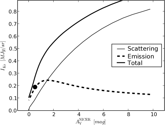
Figure 10: Predicted distribution of scattered and emitted radiation in the case of a spherically symmetric cloud with $A_{\rm V}=10^{\rm m}$ for the sightline through the cloud centre. The model is based on the Mathis et al. (Mathis83 (1983)) radiation field and the dust model described in Sect. 4. The emission has been scaled to correspond to the Flagey et al. (Flagey2006 (2006)) prediction calculated for $A_{\rm V}=0.5^{\rm m}$.

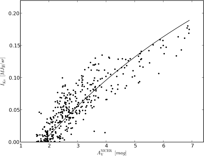
Figure 11: The observed $Ks$ intensity plotted against the extinction obtained with the NICER method. The intensities are relative to the value found in the reference region (see Fig. 2). Only points below $A_{\rm V}=7^{\rm m}$ are shown. The curve indicates the expected curvature based on numerical modelling.

In Fig. 11 we plot observed Ks intensities against extinctions calculated with the NICER method. The plotted curve represents the expected curvature of this relation (i.e., it corresponds to the value of $b_{\rm K}$ quoted above). The value was obtained from numerical modelling assuming normal dust properties. In the case of dust emission clouds should show some degree of limb brightening that, in this figure, would cause the slope to become shallower at low extinctions. There is no indication of such a trend, neither in the internal distribution of data points nor in comparison with the predicted behaviour due to scattering only. If the emission were as strong as depicted in Fig. 10, the signal at $A_{\rm V}=1.5^{\rm m}$ would be increased by almost 0.1 MJy/sr compared with the total signal at $A_{\rm V}=6^{\rm m}$. Based on Fig. 11 the contribution of dust emission must be lower by almost a factor ten. Note, however, that the prediction of Fig. 10 is based on a simple, spherically symmetric cloud with a smooth density distribution. For example, inhomogeneities or a different cloud geometry could well decrease the contrast between cloud edge and sightlines of higher extinction. Nevertheless, it is safe to say that dust emission is unlikely to interfere with the use of surface brightness as a tracer of cloud column densities.

7.2 Sampling effects in the NICER extinction maps

We noted already that the NICER values may have been affected by poor sampling of regions with strong extinction gradients. We examined this possible bias with simulated observations. As a starting point we take the map $A_{\rm V}^{\rm NICER}$ which is first interpolated to a ten times higher resolution. Background stars are simulated using the magnitude and intrinsic colour distributions obtained from observations. The simulations take into account the observed, two-dimensional probability distribution of the colours. The synthetic observations are run through the NICER routine resulting in a new extinction map. The procedure is repeated so that we obtain 100 realizations of the extinction map. In Fig. 12 the results are compared with each other and with the input $A_{\rm V}$ distribution, again using the 20$\arcsec$ resolution.

Frame a shows the original $A_{\rm V}$ distribution and the positions of the observed stars. The average recovered map (frame b) follows the true extinction distribution but within the filament the recovered extinction values are systematically too low. This is not surprising as the number of stars observed in this region is very small. The bias is plotted in frame c. The largest errors are associated with opacity gradients in optically thick regions. At the centre of the filament the errors can again decrease, as the $A_{\rm V}$ distribution flattens out. In Fig. 12c this is true especially at the lower part of the map. Frame d shows the dispersion between different realizations of the extinction map. The map shows a similar pattern, statistical errors increasing where also the systematic errors are large. The last two plots in Fig. 12 show the bias and scatter of the $A_{\rm V}$ estimates as functions of true extinction. Both systematic and statistical errors increase monotonically with $A_{\rm V}$, although it is probably significant that in our case large $A_{\rm V}$ also often corresponds to large $A_{\rm V}$ gradients. The plots extend to regions with true extinction above 25^m. However, as seen from frames a and b, above $A_{\rm V}\sim 15^{\rm m}$ the estimates mostly correspond to interpolated values between stars more than 20$\arcsec$ apart.

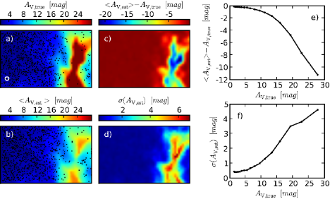
Figure 12: Simulations of estimated errors in the NICER $A_{\rm V}$ map. The $A_{\rm V}$ distribution obtained with the NICER method (frame $a$) is used as a starting point. New $A_{\rm V}$ maps are obtained by simulating stars at random locations, frame b showing the average of these. The observed stars (frame a) and an example of simulated distribution of stars (frame b) are indicated with black dots. The other images show the average bias (frame $c$), and internal dispersion (frame $d$) of the $A_{\rm V}$ estimates. The rightmost plots show the bias and the internal standard deviation of the $A_{\rm V}$ estimates as functions of true visual extinction. All maps correspond to averages weighted with a gaussian with FWHM equal to 20$\arcsec$ (the circle in frame a).

Figure 12 indicated a significant bias with respect to the input map. Therefore, one can assume that also the original NICER estimates contain similar errors. For example, when the estimated $A_{\rm V}$ value is around 15^m, the true value could well be above $20^{\rm m}$. In fact, the errors could be even slightly larger, because our simulation does not include the effect of small scale opacity variations. Therefore, this bias could explain most of the discrepancy that was seen in Fig. 8. When extinction derived from surface brightness data is around $15^{\rm m}$, the NICER method predicts values that are lower by $\sim 5^{\rm m}$.

7.3 Interstellar radiation field and variations of dust illumination

Remarkably, the surface brightness data could be converted into column densities without any assumption on the intensity or spectral shape of the local radiation field. This was because most parameters, $a_{\rm J}$, $a_{\rm H}$, and $a_{\rm Ks}$ in particular, were obtained by fitting Eq. 1 directly to observations. Only the parameter $b_{\rm Ks}$ was fixed to the value obtained from earlier model calculations. The parameter $b_{\rm Ks}$ represents mainly the Ks band optical depth and, therefore, should be independent of the intensity of the radiation field. In Juvela et al. ( Juvela2006 (2006)) $a_{\rm Ks}$ and $b_{\rm Ks}$ were fitted simultaneously and, because the functional form is not perfect in describing the observed relation between surface brightness and column density, a change in the radiation field could slightly affect also the parameter $b_{\rm Ks}$. The effect should be small and, therefore, we can assume that the column density estimates presented in this paper are effectively independent from the radiation field assumed in Juvela et al.( Juvela2006 (2006)).

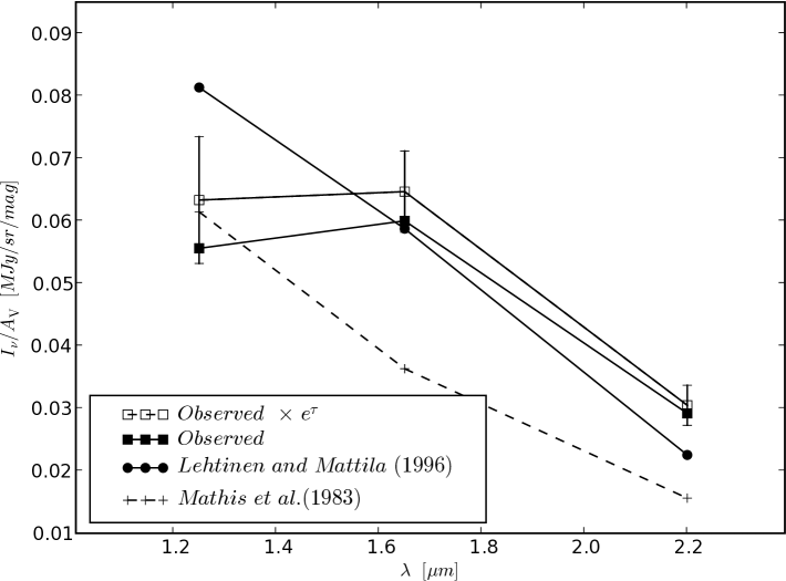
Figure 13: Observed and predicted intensities of scattered light per unit visual extinction. The observed spectrum (filled squares) corresponds to fits to surface brightness against NICER estimated visual extinction. The uppermost curve (open squares) is obtained by multiplying these with $e^{\tau}$, where $\tau$ corresponds to the expected attenuation surrounding the filament. The other curves show spectra of scattered light assuming either Mathis et al. (Mathis83 (1983)) or Lehtinen et al. (Lehtinen1996 (1996)) radiation field, and normal dust scattering properties (see text).

If the ratios between the scattering cross sections of all bands are assumed to be known, observations of optically thin sightlines give the spectrum of the illuminating radiation field. Because we have already estimated visual extinctions, we can estimate also the absolute intensities. In Figure 13 we compare the observed surface brightness values with predictions, assuming the normal dust properties used in this paper (see Sect. 4). For the observations we plotted surface brightness against NICER estimates of $A_{\rm V}$. Linear fits were made to data where optical depth in the corresponding band was below 0.7. Figure 13 shows the slopes, which represent the intensity of the illuminating radiation field. We should further take into account the fact that in our ON field the minimum $A_{\rm V}$ value is $\sim$1.8 magnitudes. If the cloud is surrounded by an isotropic attenuating layer, the true ISRF outside this layer should be higher by a factor of $e^{\tau_{\nu}}$, where $\tau_{\nu}$ is the corresponding NIR optical depth. In reality the effect is decreased because of the strong forward scattering in the NIR. We assume effective $\tau_{\nu}$ values corresponding to $\sim$0.5 magnitudes of visual extinction. The resulting ISRF estimates are shown in Fig. 13 with open squares. The error bars have been calculated with the bootstrap method.

In Fig. 13 we plot also slopes corresponding to the Mathis et al. (Mathis83 (1983)) radiation field, i.e., the values obtained by multiplying the given Mathis et al. intensity estimates with the scattering cross sections of the Draine dust model. Based on COBE/DIRBE NIR data Lehtinen & Mattila (Lehtinen1996 (1996)) presented improved estimates of NIR ISRF. Compared with Mathis et al. those ISRF values and, consequently, the expected surface brightnesses are larger by roughly one half.

The spectrum of scattered light in Corona Australis is rather similar to what is expected for a cloud illuminated by normal ISRF. The H and Ks intensities are larger than the values given by Lehtinen & Mattila. However, the difference is significant only in the Ks band where the observed value is about 35% ($\sim$ 2 $\sigma$) larger. This cannot be an indication of additional component of dust emission in that band, because the spectrum is based on differential measurements of surface brightness in regions with $A_{\rm V}\sim 1.8^{\rm m}$ or higher. Dust emission would peak around the lowest $A_{\rm V}$ values and, therefore, would decrease rather than increase the slope in the relation of surface brightness vs. visual extinction. Between the J and Ks bands the shape of the observed spectrum is very close to both ISRF models. The J band intensity is relatively lower and quite close to the Mathis et al. value. Because of the larger error estimates, the difference to the Lehtinen & Mattila value amounts only to 1.5 $\sigma$. A correction $e^{\tau_{\nu}}$ corresponding to a $A_{\rm V}=1.5^{\rm m}$ would be enough to remove this difference. A larger correction would be justifiable, because the filament is optically thick and blocks practically all incoming radiation from that direction. Therefore, the shape of the ISRF may be close to that predicted by the models mentioned. However, with the possible exception of the J band the intensity is higher than predicted by the two ISRF models. Had we used in the correlations $A_{\rm V}$ values estimated based on the surface brightness instead of the NICER estimates, the intensity difference would further increase by $\sim$10% (see Fig. 8).

In Fig. 13 the ISRF models were converted into expected surface brightness of scattered light using the Draine dust model. In the model the albedos are close to the lower limit of the range that Lehtinen & Mattila (Lehtinen1996 (1996)) derived from NIR observations. In Fig. 13 larger albedo values would move the Mathis et al. and the Lehtinen & Mattila ISRF curves upwards in the same proportion. In the NIR the scattering is also mostly in the forward direction and the intensity of the scattered light should depend more on the radiation coming in from behind the cloud than on the average intensity over the whole sky. In the Draine dust model the asymmetry parameter of scattering, $<cos\theta>$, is 0.28 for the J band and 0.13 for the K band. Using the DIRBE zodiacal light subtracted all-sky maps at 1.25 $\mu$m and 2.2 $\mu$m one can estimate that the scattered surface brightness of the Corona Australis cloud should be 20-30% higher than what would be expected based on the average sky brightness alone. Therefore, the strong forward scattering can also explain why the ISRF estimate in Fig. 13 is above the two models.

The star R Corona Australis lies only some five arc minutes East of our field. In the visual (see Fig. 1) the associated reflection nebula does not extend near our ON field, but in NIR the star could have a significant effect at that distance. The intervening extinction cannot be determined. If the star is sufficiently far in the foreground, it could illuminate also the Northern side of the filament. In the 2MASS catalog R Corona Australis has observed magnitudes of 6.9, 5.0, and 2.9 in J, H, and K, respectively (Cutri et al. Cutri2003 (2003)). Assuming a distance of 130 pc (Marraco & Rydgren Marraco81 (1981)) the projected distance between R CrA and the centre of our field is $\sim$0.5 pc. If we assume that the extinction between R CrA and the observed field is similar to the extinction between between R CrA and us, the resulting ratio of energy densities produced by R CrA and the Mathis ISRF would be 0.05, 0.18, and 0.94, for J, H, and K. In other words, in the Ks band R CrA could affect the Ks intensities while in the J band it should have only little influence. However, the relation between $I_{\rm K}$ and $A_{\rm V}^{\rm NICER}$ does not indicate any gradient in ISRF across the field from East to West.

According to Fig. 11, observed Ks intensities are below the predicted curve when extinction exceeds 4–5^m. The effect may be a direct indication of the shadowing produced by nearby optically thick regions. As was seen in Fig. 6, the sightlines with $A_{\rm V}>5^{\rm m}$ are already quite close to the filament. The effect is not visible in Fig. 5 because there the corresponding curves were fitted to surface brightness data without knowledge of an absolute $A_{\rm V}$ scale. The effect could mean that column densities are underestimated for the corresponding lines-of-sight. However, this conclusion is not supported by the correlation in Fig. 8 where, at high extinctions, the NICER method tends to predict lower extinction values.

Because of the differences in the radiation field and its attenuation by the dense parts of the cloud the same parameters that were successfully used to translate surface brightness into column density on the northern side, may not work equally well on the southern side. In Sect. 6 only column density estimates north of the filament were discussed. However, Figs. 6 and 7 show that on the southern side the surface brightness method has predicted significantly higher column densities than the NICER method. This is just an indication that the parameter values employed in the surface brightness method are not global constants and that, in the case of optically very thick structures, changes can take place over short distances. Isotropic radiation field and optical depths below $A_{\rm V}\sim 20^{\rm m}$ were quoted as pre-requisites for reliable conversion between surface brightness and column density. Our field is clearly in contradiction of both rules. Nevertheless, in the region where the necessary parameters could be determined the method was found to give reliable estimates. For very optically thick regions like the central part of the imaged filament, the simple approach used in this paper is not sufficient. In those cases numerical modelling of the surface brightness observations may be required to improve the accuracy of the estimates.

7.4 Comparison with millimetre emission data

Some information on the column densities for the centre of the filament comes from Chini et al. (Chini2003 (2003)) who observed the R Corona Australis cloud in 1.2 mm continuum with the SIMBA instrument. The signal-to-noise ratio is not high enough so that much structure could be seen in the region now observed in NIR. However, in Fig. 2 of Chini et al. a local emission maximum, consisting of millimeter sources MMS2 and MMS3, does coincide with our region $e$. It is doubtful whether MMS2 and MMS3 are truly separate clumps or whether their apparent division is caused by noise. Chini et al. do not suggest that they would represent protostellar condensations. The sources reside within a larger emission peak that agrees with the position of region $e$ and confirms the presence of a local column density maximum there. The intensity of the mm emission is $\sim$160 mJy per 28$\arcsec$ beam. Using the parameters suggested by Chini et al., a mass absorption cross section $\kappa=0.37$cm²g^-1 and a gas-to-dust ratio of 150, this corresponds to a beam averaged hydrogen column density of $N({\rm H}_{2})$=3.8$\times 10^{22}$cm^-2. Using the standard relation given by Bohlin et al. (Bohlin78 (1978)), this corresponds to a visual extinction of $A_{\rm V}$=40^m. This is at least consistent with the observed scattered light, which indicates an extinction well above 20 magnitudes. As mentioned, a more quantitative value (or a strict lower limit) to $A_{\rm V}$ will be derived from the NIR surface brightness data in a future paper with the help of radiative transfer modelling. Figure. 1 of Chini et al. further indicates the presence of higher column densities some distance to the west, coinciding with the region $f/g$. Therefore, although the NIR scattered light suffers from significant saturation, it is still able to point out the most opaque regions and give some information on their small scale structure.

In the SIMBA observations of Chini et al. the effective mapping rate was $\sim$1.8 min per square arc minute which resulted in an 1-$\sigma$ noise of 17 mJy per beam. Observations of an area similar to our NIR mapping, $4\arcmin\times 8\arcmin$, took approximately one hour. Assuming a dust temperature of 16 K the SIMBA sensitivity corresponds to $A_{\rm V}\sim 3^{\rm m}$ at the resolution of 24$\arcsec$. Based on Fig. 8 the internal scatter in our NIR data corresponds at low extinctions to $A_{\rm V}\sim 0.5-1.0^{\rm m}$. The lower value may be closer to the truth because, as discussed in Sect. 6.1, most of the scatter appears to come from the colour excess method. Adjusting for the difference in resolution and sensitivity, a SIMBA type instrument would need between 13 and 52 hours of observing time to reach similar accuracy. In other words, with similar observing times similar accuracy could be reached with both the NIR and mm instruments.

Compared with SIMBA the new generation of sub-millimeter bolometers, LABOCA and SCUBA-II among the first, will significantly increase the efficiency of dust emission observations at long wavelengths. However, similar improvement is taking place in NIR instrumentation. As an example, the VIRCAM instrument on ESO’s VISTA telescope has an instantaneous field-of-view that is two orders of magnitude larger than that of the SOFI instrument. The NIR and sub-mm/mm wavelength observations remain largely complementary, especially regarding the range of $A_{\rm V}$ they cover. However, with sufficiently long integrations, the NIR scattering can provide maps with significantly higher resolution.

8 Conclusions

We have made deep near-infrared observations of a cloud filament in the Corona Australis molecular cloud. The goal was to detect NIR scattered light towards the cloud and to confirm that this surface brightness can be used to derive reliable column density maps. The column density estimates were made using methods presented by Padoan et al. (Padoan2006 (2006)) and Juvela et a. (Juvela2006 (2006)). The photometry of the background stars and the NICER method were used to derive an independent extinction map.

Our results show that

• Surface brightness could be detected over most of the imaged fields where, according to the NICER analysis, the $A_{\rm V}$ ranges from $1.8^{\rm m}$ to more than $30^{\rm m}$.

• The NIR intensities and their $A_{\rm V}$ dependencies are consistent with the surface brightness being caused by dust scattering. No clear indication of additional dust emission at low $A_{\rm V}$ was detected.

• In regions below $A_{\rm V}\sim 15^{\rm m}$ the column density estimates derived using scattered light and the colour excesses of background stars agree with each other.

• In our case the surface brightness data allow construction of a column density maps with resolution a few times better than that provided by the background stars.

• In the interval $A_{\rm V}=15-20^{\rm m}$ the surface brightness data predicts up to 50% higher extinction values than the colour excess method. We interpret this as bias in the colour excess method caused by the strong extinction gradients and the small number of background stars.

• The absence of background stars prevents the NICER method from providing reliable estimates for the extinction at the centre of the filament. The morphology of surface brightness maps is still able to point out local extinction maxima. However, quantitative estimates of $A_{\rm V}$ (or its lower limits) will require modelling of the cloud and the radiation field.

The results show that near-infrared scattering can be used for mapping of quiescent interstellar clouds. The changes in dust grain properties within dense clouds and small scale variations in the gas-to-dust ratio remain possible sources of uncertainty when any dust tracers are used to infer the distribution of total cloud mass (e.g. Padoan et al. Padoan2006 (2006)). On the other hand, by providing high resolution images of the dust distribution the near-infrared scattering also provides a useful tool for the study of these questions.

Appendix A NIR correlations

Figure 14 shows correlations between the observed J and H and the H and K surface brightness values. The regions that were identified in Fig. 4 are also here plotted with different symbols. The regions $c$–$g$ correspond to distinct areas in all correlations. This indicates that the spectra of scattered light are to some extent anomalous in these regions (see Sect. 3). On the other hand, regions $a$ and $b$ are separated clearly only along the K–axis. This suggest that they could be caused by observational effects, i.e., an artificial gradient in the K band image.

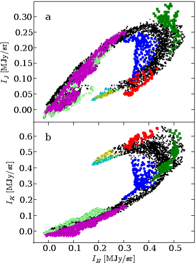
Figure 14: Correlations between the observed NIR surface brightness values. The plots complement Fig. 4 that showed the remaining correlations between the J and H bands (frame a) and H and K bands (frame b).

Similar effects are seen in the off fields where the expected signal from dust should be negligible. Figure 15 shows for the field OFF1 the colour 0.8$\times$J-K after stars have been removed using a median filter of 50$\times$50 pixels. At the image borders there are systematic colour variations at a level of close to 0.1 MJy sr^-1, i.e. at a level comparable to the regions $a$ and $b$. This could be caused, e.g., by an imperfect illumination correction. In our analysis the image borders were masked out. However, border effects in individual frames could still explain some of the features seen in Fig. 4 because the jitter pattern was larger than the width of the rejected borders. In this respect the analysis could still be improved by applying a mask already to individual frames instead of the final image.

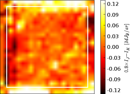
Figure 15: The colour 0.8$\times$J-K in the field OFF1 after stars have been removed with median filtering. The image shows some systematic colour variations at the image borders. The box indicates the extent of the image borders that in our analysis was mask out.