An Isochrone Database and a Rapid Model for Stellar Population Synthesis

Abstract

We first presented an isochrone database that can be widely used for stellar population synthesis studies and colour-magnitude diagram (CMD) fitting. The database consists of the isochrones of both single star and binary star simple stellar populations (ss-SSPs and bs-SSPs). The ranges for the age and metallicity of populations are 0–15 Gyr and 0.0001–0.03, respectively. All data are available for populations with two widely used initial mass functions (IMFs), i.e., Salpeter IMF and Chabrier IMF. The uncertainty caused by the database (about 0.81%) is designed to be smaller than those caused by the Hurley code and widely used stellar spectra libraries (e.g., BaSeL 3.1) when the database is used for stellar population synthesis.

Then based on the isochrone database, we built a rapid stellar population synthesis ($RPS$) model and calculated the high-resolution (0.3 $\rm{\AA}$) integrated spectral energy distributions (SEDs), Lick indices and colour indices for bs-SSPs and ss-SSPs. In particular, we calculated the $UBVRIJHKLM$ colours, $ugriz$ colours and some composite colours that consist of magnitudes on different systems. These colours are useful for disentangling the well-known stellar age–metallicity degeneracy according to our previous work.

As an example for applying the isochrone database for CMD fitting, we fitted the CMDs of two star clusters (M67 and NGC1868) and obtained their distance moduli, colour excesses, stellar metallicities and ages. The results showed that the isochrones of bs-SSPs are closer to those of real star clusters. It suggests that the effects of binary interactions should be taken into account in stellar population synthesis. We also discussed on the limitations of the application of the isochrone database and the results of the $RPS$ model.

1 Introduction

Stellar population synthesis is a widely used technique to model the spectra and photometry evolution of galaxies. It is also an important method to estimate the stellar contents of galaxies from spectra (e.g., Trager et al. 2000) or photometry data (e.g., Li et al. 2007; Li & Han 2007b). A lot of models such as Bruzual & Charlot (2003) (GALAXEV), Worthey (1994), Vazdekis (1999) , Fioc & Rocca-Volmerange (1997) (PEGASE), and Zhang et al. (2005) have been brought forward for studying stellar populations, but most of them did not take binary interactions into account. Similarly, the popular models for galaxy formation and evolution (e.g., Baugh et al. 1998, Cole et al. 2000, De Lucia et al. 2006) did not take binary interactions into account, either. Therefore, most results of stellar population studies are derived from single star stellar population (ss-SSP) models, e.g., Terlevich & Forbes (2002), Gallazzi et al. (2005), Trager et al. (2000), while only a few results from binary star stellar population (bs-SSP) model (Li et al., 2006). A reason for those works using ss-SSPs rather than bs-SSPs is that the evolution of binaries is much more complicated than single stars. The calculation of binary stellar population synthesis usually takes much more time and disk space compared to single stellar population synthesis. However, as pointed out by, e.g., Han et al. (2001), Zhang et al. (2004), more than 50% stars are in binaries, and binary interactions are important for stellar population synthesis. Many observational phenomena such as the Far-UV excess of elliptical galaxies (Han et al., 2007) and blue stragglers in star clusters (Tian et al. 2006; Xin et al. 2007) can be explained more naturally via bs-SSPs than via ss-SSPs. In fact, both blue stragglers and Far-UV excess of elliptical galaxies can be produced naturally by binary interactions without any special assumptions (see Han et al. 2007 for more details). This suggests that it is necessary to model stellar populations of galaxies via bs-SSPs. We mainly intend to build a database for stellar population synthesis studies and present a new model for quickly modeling bs-SSPs.

The structure of the paper is as follows. In Sect. 2, we briefly introduce the evolution of stars. In Sect. 3, we present the isochrone database for stellar population synthesis studies. In Sect. 4, we present our new stellar population synthesis model. As an application of the isochrone database in colour-magnitude diagram (CMD) studies, we fit the CMDs of two star clusters in Sect. 5. Finally, we give our discussions and conclusions in Sect. 6.

2 Evolution of stars

In this work, we use the rapid stellar evolution code of Hurley et al. (2002), hereafter Hurley code, to evolve binaries and single stars. This code enables modeling of even the most complex binary systems. Binary interactions such as mass transfer, mass accretion, common-envelope evolution, collisions, supernova kicks, angular momentum loss mechanism, and tidal interactions are considered (see Hurley et al. 2002 for details). Besides the code can calculate the evolution of stars quickly, the average uncertainty caused by the code is typically smaller than 5%.

3 The isochrone database

3.1 Input parameters

To build a database for conveniently and quickly modeling stellar populations, we take wide ranges for input stellar-population parameters (metallicity, $Z$; age, $t$; initial mass function, IMF). In detail, 0.0001–0.03 and 0–15 Gyr are taken for the ranges of $Z$ and $t$, respectively, and two widely used IMFs are taken in the work. The two IMFs are presented by Salpeter (1955) and Chabrier (2003) respectively and are listed in Table 1.

Table 1: The IMFs adopted in this work.

IMF name	IMF expression	Example models
Salpeter	$\phi(m)\propto$ $m^{-2.35}$	Worthey (1994), Zhang et al. (2005)
Chabrier	$\phi({\rm log}~{}m)\propto\left\{\begin{array}[]{ll}\exp[{{(\log m-\log m_{\rm c})^{2}}\over{-2\sigma^{2}}}],~{}~{}(m\leq 1M_{\odot};~{}m_{\rm c}=0.08M_{\odot},\sigma=0.69)\\ \\ m^{-1.3}~{}~{}(m>1M_{\odot})\end{array}\right.$	Bruzual & Charlot (2003)
Note: The mass of each star is given between 1 and 100 $M_{\odot}$ in this work, as Bruzual & Charlot (2003).

We use a Monte Carlo method to generate the binary sample of bs-SSPs. For each binary, we generate the masses of two components ($M_{\rm 1}$ and $M_{\rm 2}$), the separation between the two components ($a$), and the eccentricity of the binary ($e$). For ss-SSPs, we just evolve stars independently. Therefore, the bs-SSPs and ss-SSPs have the same star sample. We take the same distribution as Mazeh et al. (1992) and Goldberg & Mazeh (1994) for $q$, and a distribution as Han et al. (1995) for $a$. The detailed process for generating the input parameters is as follows.

First, we generate the mass of the primary, $M_{\rm 1}$, within the range of 0.1–100 $M_{\odot}$, according to an IMF. Next we generate the ratio ($q$) of the mass of the secondary to that of the primary randomly within 0–1, due to an a uniform distribution

$$p(q)=1,~{}~{}0\leq q\leq 1,$$ (1)

where $q=M_{\rm 2}/M_{\rm 1}$. Then the mass of the secondary star is given by $q$.$M_{\rm 1}$. One can also refer to Zhang et al. (2004).

Second, we generate the separation ($a$) of two components of a binary following the assumption that the fraction of binary in an interval of log($a$) is constant when $a$ is big (10$R_{\odot}$ $<a<$ 5.75 $\times$ 10⁶$R_{\odot}$) and it falls off smoothly when when $a$ is small ($\leq$ 10$R_{\odot}$). The distribution of $a$ can be written as

$$a~{}.p(a)=\left\{\begin{array}[]{ll}a_{\rm sep}(a/a_{\rm 0})^{\psi},&~{}a\leq a_{\rm 0}\\ a_{\rm sep},&~{}a_{\rm 0}<a<a_{\rm 1}\\ \end{array}\right.$$ (2)

where $a_{\rm sep}\approx 0.070,a_{\rm 0}=10R_{\odot},a_{\rm 1}=5.75\times 10^{\rm 6}R_{\odot}$ and $\psi\approx 1.2$. This distribution implies that about 50% (the typical value of the Galaxy, see Han et al. 1995) of stars are in binaries with orbital periods less than 100 yr.

Third, we generate the eccentricity ($e$) of each binary system using a uniform distribution, in the range of 0–1, as Zhang et al. (2004). Actually, the distribution of $e$ affects the stellar population synthesis results slightly, according to Zhang et al. (2004).

3.2 Building of the database

To build an useful database for stellar population synthesis, the isochrone database has to contain all the data needed in stellar population synthesis. Three stellar-evolution parameters (effective temperature, $T_{\rm eff}$, surface gravity, log($g$), and luminosity, log($L/L_{\odot}$)) of stars in populations are important for stellar population synthesis and we include them into the database. In the work, each stellar population consists of 2 000 000 binaries or 4 000 000 single stars. In fact, the sample contains two times of stars in the sample of Zhang et al. (2005) and some satisfying population synthesis results can be obtained via such a sample (see Zhang et al. 2005 for more details). To make the library can be used combining with most widely used spectra libraries to calculate the integrated specialities such as spectral energy distributions (SEDs) and magnitudes of stellar populations, we take wide ranges for the stellar-evolution parameters. The ranges are wider than those of most stellar spectra libraries, e.g., BaSeL 3.1 (Westera et al., 2002), STELIB (Le Borgne et al., 2003), and the library of Delgado et al. (2005). In detail, our results are presented within the range of 2 000 – 60 000 K for $T_{\rm eff}$, and -1.5 – 6 for log($g$).

To save disk space, the stellar-evolution parameters of stellar populations are given by a statistical method. In other words, the database supplies us with approximate distributions of stars in the log($g$) versus $T_{\rm eff}$ grid (hereafter $gT$-grid), i.e., approximate isochrones, rather than the stellar-evolution parameters of each star. The detailed procedure is as follows. First, we divide $gT$-grid into 1 089 701 sub-grids, with intervals of 0.01 and 40 K for log($g$) and $T_{\rm eff}$, respectively. The two intervals lead to an average uncertainty of 0.81% in stellar population synthesis results, which is smaller than those caused by the Hurley code (5%) and most stellar spectra libraries (e.g., 3–5% for BaSeL 3.1). Therefore, our results is accurate enough for most stellar population synthesis studies. Second, for each stellar population, we count the stars locate in each sub-grid, and save the median log($g$), median $T_{\rm eff}$, average log($L/L_{\odot}$) and percentage of stars in the sub-grid. The reason for saving the median values rather than the average values of log($g$) and $T_{\rm eff}$ is that the two kinds of values lead to almost the same stellar population synthesis results but each pair of median log($g$) and $T_{\rm eff}$ corresponds to a fixed sub-grid of the $gT$-grid and they can be used more conveniently in stellar population synthesis studies. The four parameters can describe the isochrones and Hertzsprung–Russell diagrams (HRDs) of stellar populations. They can also be used for calculating the average surface area of stars in each sub-grid.

3.3 The database

As a whole, the isochrone database contains the distributions of $T_{\rm eff}$, log($g$), and log($L/L_{\odot}$) of stars, i.e., isochrones of bs-SSPs and ss-SSPs. The age range for the database is 0–15 Gyr, with an interval of 0.1 Gyr, and the metallicity range is 0.0001–0.03 (0.0001, 0.0003, 0.001, 0.004, 0.01, 0.02 and 0.03). In special, the data for stellar populations with Salpeter and Chabrier IMFs are presented. The database can be used to model the CMDs of star clusters and calculate the integrated specialities of stellar populations. The database can be obtained by on request to the authors or via the CDS in the future.

To understand the database more expediently, we show the isochrones of metal-poor ($Z$=0.0001), solar-metallicity ($Z$=0.02) and metal-rich ($Z$=0.03) stellar populations in Figs. 1, 2 and 3, respectively. The populations here have Salpeter IMF. Note that we take stellar populations with Salpeter IMF as our standard models and we only show the results for standard models in the whole paper. In the figures, both the isochrones of bs-SSPs and ss-SSPs are shown, which can help us to understand the effects of binary interactions on stellar population synthesis. We see clearly that the isochrones of bs-SSPs are different significantly from those of ss-SSPs. We will find that the isochrones of bs-SSPs are closer to those of star clusters when we fit the CMDs of two star clusters later.

Figure 1: Isochrones for binary stellar populations (bs-SSPs) and single stellar populations (ss-SSPs) with metallicity of 0.0001 and Salpeter IMF. Symbols “bs” and “ss” denote bs-SSP and ss-SSP, respectively. The points show only the range of the distribution rather than the number of stars.

Figure 2: Similar to Fig.1, but for stellar populations with metallicity of 0.02.

Figure 3: Similar to Fig.1, but for stellar populations with metallicity of 0.03.

4 Rapid population synthesis model

The isochrone database above enables quickly calculating the spectral energy distributions (SEDs) of stellar populations, and then the Lick Observatory Image Dissector Scanner indices (Lick indices) and colour indices. Besides the method does not need to evolve each star, it computes only one time for the spectra of stars in each sub-grid of the $gT$-grid. Therefore, via such technique, we can calculate the integrated peculiarities of stellar populations very quickly. We call this stellar population synthesis technique and model rapid stellar population synthesis ($RPS$). It actually takes much less (about one of 100 000) time than the method used by, e.g., Zhang et al. (2005). Therefore, the $RPS$ method makes it more convenient to take binary interactions into account when modeling the formation and evolution of galaxies. In the work, we calculated the SEDs, Lick indices and colour indices for bs-SSPs and ss-SSPs. They can be conveniently used for future studies.

4.1 SEDs and Lick indices

We calculated the SEDs and 25 widely used Lick indices for bs-SSPs and ss-SSPs with two IMFs. The high-resolution stellar spectra library of Martins et al. (2005) (hereafter Martins library) was used for the work. The library was computed with the latest results of stellar atmospheres studies and covers a $T_{\rm eff}$ range from 3 000 to 55 000 K and a log($g$) range from -0.5 to 5.5. In particular, the library enables modeling the spectra of stellar populations at a 0.3 ${\rm\AA}$ resolution. Thus the library is suitable for spectral studies of stellar populations of galaxies and star clusters. However, the metallicity coverage of the library is only from 0.002 to 0.04. In Figs. 4, 5 and 6, we show the SED evolution of bs-SSPs with metallicities of 0.004, 0.02 and 0.03, respectively. As we see, as that of ss-SSPs (see, e.g., Bruzual & Charlot 2003), the continuum trends to be redder with increasing age of bs-SSP and the metallicity of bs-SSP affects the metal line (e.g., Fe lines with central wavelengths of 5270 and 5335 ${\rm\AA}$) strengths obviously. We can also check the effects of stellar age and metallicity via some Lick indices. In Figs. 7, 8, 9 and 10, we plotted the evolution of four widely used Lick indices. The indices shown are computed from SEDs with a 0.3 ${\rm\AA}$ resolution, but we also calculated the indices on the Lick system. Note the work calculates the Lick indices of populations from SEDs, but Zhang et al.’s works calculate the indices on the Lick system using some fitting functions. The figures (7, 8 and 9) show that the stellar metallicity affects the age-sensitive line index H$\beta$ slightly, while it affects metallicity-sensitive indices (Mgb, Fe5270, and Fe5335) strongly, and the stellar age changes the H$\beta$ index similarly for populations with various metallicities. Therefore, the line indices of bs-SSPs have similar age and metallicity sensitivities as those of ss-SSPs. This suggests that when we take bs-SSP models instead of ss-SSP models to study the stellar populations of galaxies, we can use H$\beta$ together with [MgFe] (Thomas et al., 2003) to give estimates for the age and metallicity of populations. To check the reliability of our $RPS$ technique, we also plotted the results derived by Zhang et al. (2005) in Figs. 7, 8, 9 and 10. The two models took the same IMF, stellar evolution code and spectra library, and both of them are bs-SSP models, but their age ranges, star samples and computing method are different. It is shown that the $RPS$ model gave line indices similar to those of the previous work, but the indices obtained by this work evolve more smoothly. The reason is that we take 2 000 000 binaries for a bs-SSP in the work but it is 1 000 000 in the previous work. Note that we obtained different metal indices for bs-SSPs with metallicity of 0.01. The reason is as follows. The Martins library supplies the same set of spectra for stars with metallicities ([$Z$/H]) of -0.3 and -0.5. We took the set of spectra as the spectra of stars with [$Z$/H] = -0.3, but the same set of spectra were taken as the spectra of stars with [$Z$/H] = -0.5 in the work of Zhang et al. (2005), when calculating the SEDs of populations with metallicity ($Z$) of 0.01. The good consistency of our results with those of the previous work suggests that our isochrone database can be used reliably for stellar population studies. Furthermore, we find that the abrupt change of indices between 1 and 2 Gyr are possibly caused by the ’phase’ transitions of stars with initial mass between about 1.57 and 2 $M_{\rm\odot}$. Such stars are in core helium burning stage and have high luminosities between 1 and 2 Gyr. As a result, it leads to a irregularity in the line indices and colours (see Bruzual & Charlot 2003 for comparison). However, the values of indices in the age range are possibly affected by the rough calculation of the evolution of stars by the Hurley code.

Figure 4: Evolution of spectral energy distributions (SEDs) of metal-poor ($Z$ = 0.004) bs-SSPs. Note that the y-axes of four panels are valued independently.

Figure 5: Similar to Fig.4, but for solar-metal bs-SSPs.

Figure 6: Similar to Fig.4, but for metal-rich ($Z$ = 0.03) bs-SSPs.

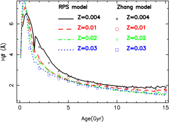
Figure 7: Comparison of the H$\beta$ index obtained by this work with those by Zhang et al. (2005). The indices are computed from SEDs directly. $RPS$ indicates our model. The two models are bs-SSP model.

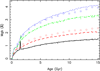
Figure 8: Similar to Fig. 7, but for Mgb.

Figure 9: Similar to Fig. 7, but for Fe5270.

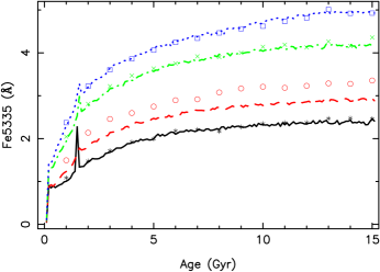
Figure 10: Similar to Fig. 7, but for Fe5335.

4.2 Colour indices

A few works have tried to model the populations of galaxies and star clusters via bs-SSPs (e.g., Zhang et al. 2004, 2005), but there is no near-infrared colour indices presented. In fact, such colours are very important for disentangling the well-known degeneracy (Worthey, 1994) and useful for exploring the stellar populations of distant galaxies (see, e.g., Li et al. 2007; Li & Han 2007b). In addition, the colours obtained by previous works (e.g., Zhang et al. 2004) do not evolve smoothly. In this work, we calculated some colours that are potentially useful for stellar population studies. The BaSeL 3.1 spectra library (Westera et al., 2002) was used for calculating the colours of populations because the wavelength coverage of Martins library is only from 3 000 to 7 000 $\rm\AA$. Note that we take a different method to calculate the colours of populations compared to the works of Zhang et al. (2004, 2005). The colours in our work are calculated by integrating SEDs, rather than by interpolating a photometry library (see Zhang et al. 2004, 2005).

4.2.1 $UBVRIJHKLM$ colours

The Johnson $UBVRIJHKLM$ colours are usually used for stellar population studies. We calculated them for both bs-SSPs and ss-SSPs with Salpeter and Chabrier IMFs. As an example, we plot the evolution of four colours of bs-SSPs with Salpeter IMF in Fig. 11. As we see, colours increase quickly with stellar age when the age is less than about 2 Gyr and then they evolve slowly. The reason is that the colours of young populations are dominated by massive stars, which evolve very quickly before about 2 Gyr. On the other hand, the colours of old ($>$ 2 Gyr) populations are mainly dominated by less massive stars, which evolve more slowly than massive stars. The figure shows that at fixed metallicity, colours become redder with increasing age. At fixed stellar age, colours become redder with increasing stellar metallicity. Therefore, the stellar age and metallicity have similar effects on colours of stellar populations. This is very the well-known age-metallicity degeneracy. Therefore, it is impossible to disentangle the effects of stellar age and metallicity completely. We can not give reliable estimate for stellar age or metallicity using only one colour. However, using a pair of colours, some constraints on the two stellar-population parameters can be obtained, because the age and metallicity sensitivities of each colour are usually different (Li & Han, 2007a). Compared to the results of Zhang et al. (2004), the colours calculated by this work evolve more smoothly. We do not compare them here, as this can be understood from the comparison of Lick indices. This is actually the first work to calculate colours relating to near-infrared bands (e.g., $V-K$ and $I-K$) for bs-SSPs. Note that $(B-V)$ is sensitive to stellar age while $(V-K)$ and $(I-K)$ to metallicity (see Li & Han 2007a).

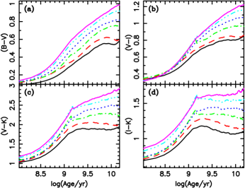
Figure 11: Evolution of four $UBVRIJHK$ colours of bs-SSPs with the Salpteter IMF. The bottom solid, dashed, dash-dotted, dotted, dash-dot-dot-dot and top solid lines are for metallicities of 0.0003, 0.001, 0.004, 0.01 and 0.02 and 0.03, respectively.

4.2.2 $ugriz$ colours

The Sloan Digital Sky Survey (SDSS) supplies a good deal of observational data for astronomy studies and it takes an $ugriz$ system (hereafter SDSS-$ugriz$ system). In order to use its photometry data for stellar population studies more conveniently, we calculated some colours on the SDSS-$ugriz$ system. In Fig. 12, we show the evolution of four colours. We see that SDSS-$ugriz$ colours have similar peculiarities as $UBVRIJHKLM$ colours. Note that colour $(u-r)$ is an age-sensitive colour and can be used to give constraints on stellar-population parameters together with colours such as $(r-K)$ (Li & Han, 2007a). This is the first work to present the SDSS-$ugriz$ colours for bs-SSPs.

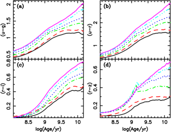
Figure 12: Similar to Fig. 11, but for four SDSS-$ugriz$ colours.

4.2.3 Composite colours

Because it is shown that some colours relating to both $UBVRIJHK$ and $ugriz$ magnitudes are more powerful than either $UBVRIJHK$ or $ugriz$ colours for disentangling the stellar age–metallicity degeneracy (Li & Han, 2007a), we computed some such colours and call them composite colours. In detail, we calculated some colours consist of Johnson $UBVRIJHK$ magnitudes and SDSS-$ugriz$ magnitudes. The evolution of four composite colours is shown in Fig. 13. According to the work of Li & Han (2007a), $(u-R)$ and $(g-J)$ are sensitive to stellar age while $(r-K)$ and $(z-K)$ to stellar metallicity.

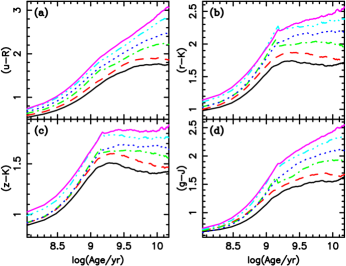
Figure 13: Similar to Fig. 11, but for four composite colours.

4.2.4 Colour pairs for disentangling stellar age–metallicity degeneracy

In this section, we show the color-color grids for two pairs of colours (hereafter colour pairs) of bs-SSPs of our standard models. The two pairs were shown to have the potential for disentangling the age–metallicity degeneracy (Li & Han, 2007a) via ss-SSPs of Bruzual & Charlot (2003). They can possibly be used to separate the stellar metallicity and age when bs-SSPs are used instead of ss-SSPs. The two pairs are [$(u-R),(R-K)$], [$(u-R),(I-K)$]. The detailed colour-colour grids of them can be seen in Figs. 14 and 15. We find that the two colour-colour grids can disentangle the age–metallicity degeneracy via bs-SSPs. Therefore, the two colour pairs can be used for stellar population studies. However, the uncertainties in stellar age and metallicity of metal-poor ($Z$ $<$ 0.001) and old (Age $>$ 12 Gyr) populations seem larger than others. Note that this two pairs are not necessarily the best pairs for stellar population study. Some other potential pairs can be found in our previous paper (Li & Han, 2007a) and it is better to choose colours according to the stellar-population peculiarities of galaxies.

Figure 14: bs-SSP grids of $(u-R)$ versus $(R-K)$. The $u$ magnitude is on the SDSS-$ugriz$ system and $RK$ magnitudes are on the Johnson system. Solid and dashed lines are for constant age and metallicity, respectively.

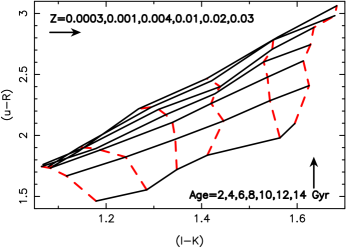
Figure 15: Similar to Fig. 14, but for $(u-R)$ versus $(I-K)$. The $I$ magnitude is on the Johnson system.

4.3 Comparison with bs-SSP model and ss-SSP model

Because most stellar population synthesis models are ss-SSP models and they have been widely used for previous works, it is necessary to compare the results (i.e., Lick indices and colours) of bs-SSP model with those of ss-SSPs. We have a try in this work. We only compare our results with those of the ss-SSPs of the model of Bruzual & Charlot (2003) (BC03 model) as most ss-SSP models gave similar Lick indices and colours for the same stellar population (see, e.g., Bruzual & Charlot 2003). The results can help us to understand how the difference between the results obtained via ss-SSP models and those obtained via bs-SSP models is. In Figs. 16 and 17, we compare four widely used Lick indices and four colours of two kinds of SSPs. Both the bs-SSP model and ss-SSP model take the Salpeter IMF and calculate their colours via BaSeL 3.1 library, but the spectra libraries used to calculate the Lick indices by two models are various. Our bs-SSP model takes the Martins (Martins et al., 2005) library and BC03 ss-SSP model mainly takes STELIB (Le Borgne et al., 2003) library. Note that the Lick indices and colours of BC03 ss-SSPs with metallicities of 0.01 and 0.03 were interpolated because they were not given directly by the BC03 model. Thus the values of the colours and Lick indices of BC03 ss-SSPs with metallicities of 0.01 and 0.03 are possibly different from those calculated by SEDs. From Fig. 16 we can find that a bs-SSP usually has larger H$\beta$ index and less metal indices than a BC03 ss-SSP when the two kinds of SSPs have the same stellar age and metallicity. We are also shown that four colours of a bs-SSP are bluer than those of an ss-SSP with the same age and metallicity. Therefore, ss-SSP models will usually measure different values for the stellar ages and metallicities of galaxies compared to bs-SSP models. However, it seems that ss-SSP models and bs-SSP models can give similar results for relative studies, because stellar age and metallicity affect Lick indices and colours of the two kinds of populations similarly.

Figure 16: Comparison of four widely used Lick indices of bs-SSPs with those of BC03 ss-SSPs. Panels a), b), c) and d) are for H$\beta$, Mgb, Fe5270, and Fe5335, respectively. Lines and points in all panels have the same meanings as in Panel a).

Figure 17: Comparison of four colours of bs-SSPs with those of BC03 ss-SSPs. Panels a), b), c) and d) are for $(B-V)$, $(V-K)$, $(I-H)$ and $(u-r)$, respectively. The $(u-r)$ colour is on the SDSS-$ugriz$ system, and the others are on the Johnson system. Lines and points have the same meanings as in Fig. 16.

5 CMD fitting for two star clusters

Besides modeling stellar populations, the isochrone database can be used for CMD fitting. Here we fitted the CMDs of star clusters M67 and NGC1868, via both bs-SSPs and ss-SSPs. The colours and magnitudes were taken from the stellar population challenge of IAU Symposium 241 (IAUS 241) (http://www.astro.rug.nl/^∼sctrager/challenge/) and the BaSeL 2.2 (Lejeune et al., 1997) spectra library was used to translate the data of our isochrone database to CMDs of stellar populations. We fitted the CMDs of the two above star clusters via stellar populations with two IMFs. First, we fitted the CMDs via populations with Salpeter IMF. As a result, via both bs-SSPs and ss-SSPs, star cluster M67 was shown to have the solar metallicity and a 4.6 Gyr age, with a distance modulus of 9.8 and a colour excess E(B-V) of 0.09. The stellar metallicity and age of NGC1868 are found to be 0.004 and 1.4 Gyr, respectively, with 18.8 for its distance modulus and 0.04 for colour excess, E(V-I). Note that we only took stellar populations with seven metallicities and 151 ages for our fittings, according to the data of our isochrone database. In the work, CMDs were fitted by comparing the theoretical and observational percentage of stars in each sub-grid of the $gT$-grid compared to the total number of stars in the observed colour and magnitude ranges. Because stars after the turn-off point are very important for determining stellar metallicity and the data of luminous stars are more reliable than those of less luminous stars, the percentage of stars in each sub-grid of $gT$-grid are weighted using their luminosities. For convenience, we using 10^(V/-2.5) instead of the real luminosities of stars. Note that $gT$-grids of populations were expressed by CMDs in the fitting. Here all stars are assumed to be distinguishable, as the limitation of the database. However, it is actually different from the true case, especially for the distant star clusters. The fittings of the CMDs of M67 and NGC1868 are shown in Fig. 18. Some sub-grids were not plotted because each of them contains less than 0.5 luminosity-weighted stars and are not important for fitting the CMDs when taking a luminosity-weighted fit method. As we see, compared to ss-SSPs, bs-SSPs can fit some special objects such as blue stragglers of M67 and as a whole, bs-SSPs fitted the shapes of the CMDs of two star clusters better. This suggests that the isochrones of bs-SSPs are closer to those of real star clusters or galaxies. It seems that SSPs can fit the CMD of M67 well, but they fit the CMD of NGC1878 not so well. The best-fit CMD of NGC1868 shows obviously different for the part with V magnitude more luminous than about 22.5 mag. This possibly results from that we assume each star of the star cluster can be distinguished but actually many stars of NGC1868 were not distinguished in observation. In fact, it is impossible to distinguish each star of the star cluster, because the star cluster is too distant (with distance modulus larger than 18). If some binary stars in the best bs-SSP-fit population of NGC1868 can not be distinguished, the CMD will be different from the one shown in Fig. 18, and it will be possibly more similar to the observational CMD. When we fitted the CMDs of the two star clusters via stellar populations with Chabrier IMF, we got similar results. It implies that even if populations with different assumptions (IMF, bs-SSP or ss-SSP) are used, we can get reliable estimates for the stellar ages and metallicities of star clusters via fitting CMDs. Note that the results of CMD fitting is usually affected by the fitting method, thus the above results are not always the best-fit results. In addition, because we only use populations with seven metallicities to fit the populations of the two star clusters, perhaps the results will change if we take populations with more metallicities for fitting.

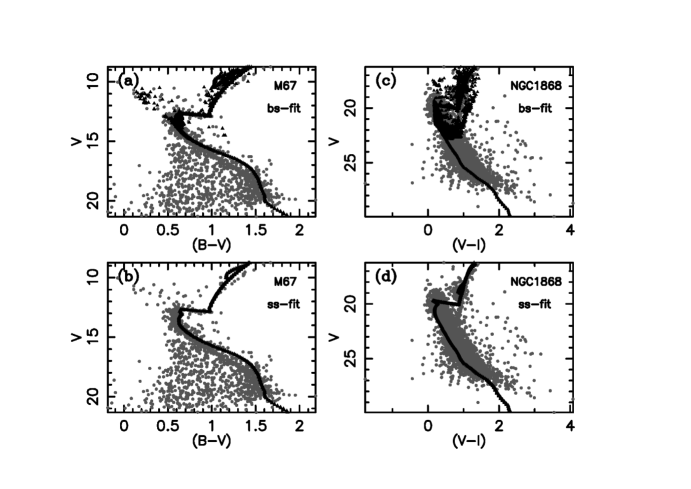
Figure 18: CMD fittings for star clusters M67 and NGC1868. Gray circles and dark triangles show the distributions of observational and theoretical stars, respectively. The upper and lower panels show the fittings via bs-SSPs and ss-SSPs, respectively. “bs-fit” and “ss-fit” mean the bs-SSP fitting and ss-SSP fitting, respectively.

6 discussions and conclusions

We first presented an isochrone database for quickly modeling both single star and binary star simple stellar populations (ss-SSPs and bs-SSPs). The isochrone database only causes 0.81% uncertainty in stellar population synthesis results on average. Thus it can be widely used for stellar population studies of galaxies and star clusters. However, there are some points should be noted when applying the database. First, because the star sample of populations was generated via Monte Carlo technique, the stellar mass distribution of a population is not continuous. As a result, some line indices and colours possibly evolve with stellar age less smoothly compared to those calculated via isochrone synthesis method (see Bruzual & Charlot 2003). This is more obvious for some near-infrared colours. Second, the isochrone database can only model stellar populations with metallicities from 0.0001 to 0.03, because the Hurley code can not evolve stars with other metallicities. In the work, we only calculated the isochrones of populations with seven metallicities (0.0001, 0.0003, 0.001, 0.004, 0.01, 0.02 and 0.03), because stars with other metallicities can not be evolved as well as stars with the above seven metallicities via Hurley code . Furthermore, the distributions of the input parameters of binaries can affect our results. In the work, we took a uniform distribution for the mass ratio of a binary, $q$, as it is the widely used distribution. However, the masses of the two components of a binary perhaps are not correlated or the distribution of $q$ is not a uniform distribution. If it is that case, we will possibly get some various results. In addition, we only present the isochrone database for two widely used IMFs, as the limitation of our computing ability. There are actually some other types for the IMF of stellar populations. We intend to study further in the future. Although we mainly aim to model simple stellar populations (bs-SSPs and ss-SSPs), the isochrone database can be used to model composite stellar populations (CSPs). The database makes it easier to study the spectra and photometry evolution of galaxies via bs-SSPs. This is useful for future studies on the formation and evolution of galaxies. It can also be used to study the effects of binary interactions on stellar population synthesis studies. In fact, to investigate how binary interactions affect the results of stellar population studies is very the topic of another work.

Then we introduced a rapid stellar population synthesis ($RPS$) model based on our isochrone database. The $RPS$ model calculated high-resolution (0.3 $\rm\AA$) spectral energy distributions (SEDs), Lick indices, and colour indices of bs-SSPs and ss-SSPs, for two widely used IMFs. However, the SEDs and Lick indices are available only for populations with metallicities of 0.004, 0.01, 0.02 and 0.03. The reason is that the metallicity coverage of the spectra library used for calculating SEDs of stellar populations is 0.002–0.04. Therefore, the metallicity range of theoretical populations is possibly not wide enough for some studies. However, $UBVRIJHK$ colours, SDSS-$ugriz$ colours and composite colours are available for populations with metallicities from 0.0003 to 0.03, which can be used to study the stellar-population parameters (age and metallicity) of most galaxies. When we compared four widely used Lick indices and four colours of bs-SSPs of RPS model to those of ss-SSPs of the BC03 model (Bruzual & Charlot 2003, BC03), we found that some various results will be shown if we take bs-SSPs instead of BC03 ss-SSPs for stellar population studies. However, it seems that even if bs-SSPs are used instead of ss-SSPs for studies, the relative values of stellar populations will not change obviously, as stellar age and metallicity affect the Lick indices and colours of bs-SSPs and ss-SSPs similarly.

Because the isochrone database can also be used to fit the colour-magnitude diagrams (CMDs) of star clusters, we fitted the CMDs of two star clusters (M67 and NGC1868) and gave their stellar metallicities, ages, distances and colour excesses, as examples. Our results showed that bs-SSPs can fit some special stars such as blue stragglers of star clusters, which can not be fitted by ss-SSPs. This suggests that one should consider binary interactions in stellar population synthesis studies. However, because the database assumes that all stars in a stellar population are distinguishable and some stars of distant star clusters can usually not be distinguished, the database is more suitable to fit the CMDs of nearby star clusters. When the database is used to fit the CMDs of very distant galaxies, one should take the above point into account.

References

- Baugh et al. (1998) Baugh C. M., Cole S., Frenk C. S., Lacey C. G., 1998, ApJ, 498, 504
- Bruzual & Charlot (2003) Bruzual G., Charlot S., 2003, MNRAS, 344, 1000
- Chabrier (2003) Chabrier G., 2003, ApJ, 586, L133
- Cole et al. (2000) Cole S., Lacey C. G., Baugh C. M., Frenk C. S., 2000, MNRAS, 319, 168
- De Lucia et al. (2006) De Lucia G., Springel V., White S. D. M., Croton D., Kauffmann G., 2006, MNRAS, 366, 499
- Delgado et al. (2005) Delgado R. M. G., Cerviño M., Martins L. P., Leitherer C., Hauschildt P. H., 2005, MNRAS, 357, 945
- Fioc & Rocca-Volmerange (1997) Fioc M., Rocca-Volmerange B., 1997, A&A, 326, 950
- Gallazzi et al. (2005) Gallazzi A., Charlot S., Brinchmann J., White S. D. M., Tremonti C. A., 2005, MNRAS, 362, 41
- Goldberg & Mazeh (1994) Goldberg D., Mazeh T., 1994, A&A, 282, 801
- Han et al. (2001) Han Z., Eggleton P. P., Podsiadlowski P., Tout C. A., Webbink R. F., 2001, Progress in Astronomy, 19, 242
- Han et al. (1995) Han Z., Podsiadlowski P., Eggleton P. P., 1995, MNRAS, 272, 800
- Han et al. (2007) Han Z., Podsiadlowski P., Lynas-Gray A. E., 2007, MNRAS, 380, 1098
- Hurley et al. (2002) Hurley J. R., Tout C. A., Pols O. R., 2002, MNRAS, 329, 897
- Le Borgne et al. (2003) Le Borgne J.-F., Bruzual G., Pelló R., Lançon A., Rocca-Volmerange B., Sanahuja B., Schaerer D., Soubiran C., Vílchez-Gómez R., 2003, A&A, 402, 433
- Lejeune et al. (1997) Lejeune T., Cuisinier F., Buser R., 1997, A&AS, 125, 229
- Li & Han (2007a) Li Z., Han Z., 2007a, MNRAS, in press, ArXiv:0704.1202
- Li & Han (2007b) Li Z., Han Z., 2007b, A&A, 471, 795
- Li et al. (2007) Li Z., Han Z., Zhang F., 2007, A&A, 464, 853
- Li et al. (2006) Li Z.-M., Zhang F.-H., Han Z.-W., 2006, ChJAA, 6, 669
- Martins et al. (2005) Martins L. P., Delgado R. M. G., Leitherer C., Cerviño M., Hauschildt P., 2005, MNRAS, 358, 49
- Mazeh et al. (1992) Mazeh T., Goldberg D., Duquennoy A., Mayor M., 1992, ApJ, 401, 265
- Salpeter (1955) Salpeter E. E., 1955, ApJ, 121, 161
- Terlevich & Forbes (2002) Terlevich A. I., Forbes D. A., 2002, MNRAS, 330, 547
- Thomas et al. (2003) Thomas D., Maraston C., Bender R., 2003, MNRAS, 343, 279
- Tian et al. (2006) Tian B., Deng L., Han Z., Zhang X. B., 2006, A&A, 455, 247
- Trager et al. (2000) Trager S. C., Faber S. M., Worthey G., González J. J., 2000, AJ, 120, 165
- Vazdekis (1999) Vazdekis A., 1999, ApJ, 513, 224
- Westera et al. (2002) Westera P., Lejeune T., Buser R., Cuisinier F., Bruzual G., 2002, A&A, 381, 524
- Worthey (1994) Worthey G., 1994, ApJS, 95, 107
- Xin et al. (2007) Xin Y., Deng L., Han Z. W., 2007, ApJ, 660, 319
- Zhang et al. (2004) Zhang F., Han Z., Li L., Hurley J. R., 2004, A&A, 415, 117
- Zhang et al. (2005) Zhang F., Li L., Han Z., 2005, MNRAS, 364, 503