Systematic ab initio study of the magnetic and electronic properties of all 3$d$ transition metal linear and zigzag nanowires

Abstract

The magnetic and electronic properties of both linear and zigzag atomic chains of all 3$d$ transition metals have been calculated within density functional theory with the generalized gradient approximation. The underlying atomic structures were determined theoretically. It is found that all the zigzag chains except the nonmagnetic (NM) Ni and antiferromagnetic (AF) Fe chains which form a twisted two-legger ladder, look like a corner-sharing triangle ribbon, and have a lower total energy than the corresponding linear chains. All the 3$d$ transition metals in both linear and zigzag structures have a stable or metastable ferromagnetic (FM) state. Furthermore, in the V, Cr, Mn, Fe, Co linear chains and Cr, Mn, Fe, Co, Ni zigzag chains, a stable or metastable AF state also exists. In the Sc, Ti, Fe, Co, Ni linear structures, the FM state is the ground state whilst in the V, Cr and Mn linear chains, the AF state is the ground state. The electronic spin-polarization at the Fermi level in the FM Sc, V, Mn, Fe, Co and Ni linear chains is close to 90% or above, suggesting that these nanostructures may have applications in spin-transport devices. Interestingly, the V, Cr, Mn, and Fe linear chains show a giant magneto-lattice expansion of up to 54 %. In the zigzag structure, the AF state is more stable than the FM state only in the Cr chain. Both the electronic magnetocrystalline anisotropy and magnetic dipolar (shape) anisotropy energies are calculated. It is found that the shape anisotropy energy may be comparable to the electronic one and always prefers the axial magnetization in both the linear and zigzag structures. In the zigzag chains, there is also a pronounced shape anisotropy in the plane perpendicular to the chain axis. Nonetheless, in the FM Ti, Mn, Co and AF Cr, Mn, Fe linear chains, the electronic anisotropy is perpendicular, and it is so large in the FM Ti and Co as well as AF Cr, Mn and Fe linear chains that the easy magnetization axis is perpendicular. In the AF Cr and FM Ni zigzag structures, the easy magnetization direction is also perpendicular to the chain axis but in the ribbon plane. Remarkably, the axial magnetic anisotropy in the FM Ni linear chain is gigantic, being $\sim$ 12 meV/atom, suggesting that Ni nanowires may have applications in ultrahigh density magnetic memories and hard disks. Interestingly, there is a spin-reorientation transition in the FM Fe and Co linear chains when the chains are compressed or elongated. Large orbital magnetic moment is found in the FM Fe, Co and Ni linear chains. Finally, the band structure and density of states of the nanowires have also been calculated to identify the electronic origin of the magnetocrystalline anisotropy and orbital magnetic moment.

I Introduction

Magnetism at the nanometer scale has been a very active research area in recent years hei00 ; pie00 ; Hern ; Hern2 , because of its novel fundamental physics and exciting potential applications. Theoretically, a great deal of research has been done on both finite and infinite chains of atoms. In particular, calculations for isotropic Heisenberg model with finite-range exchange interactions show that a one dimensional (1D) chain cannot maintain ferromagnetism at any finite temperatures. Mermin Nonetheless, this discouraging conclusion has to be revised when a magnetic anisotropy is present, as in, e.g., quasi-1D crystals. Experimentally, modern methods to prepare nanostructured systems have made it possible to investigate the influence of dimensionality on the magnetic properties. A fundamental idea is to exploit the geometrical restriction imposed by an array of parallel steps on a vicinal surface along which the deposited material can nucleate. For example, Gambardella, et al.Gambardella2 , recently succeeded in preparing a high density of parallel atomic chains along steps by growing Co on a high-purity Pt (997) vicinal surface and also observed 1D magnetism in a narrow temperature range of 10$\sim$20 K. Structurally stable nanowires can also be grown inside tubular structures, such as the Ag nanowires of micrometer lengths grown inside self-assembled organic (calix[4]hydroquinone) nanotubesSuh . Short suspended nanowires have been produced by driving the tip of scanning tunneling microscope into contact with a metallic surface and subsequent retraction, leading to the extrusion of a limited number of atoms from either tip or substrateRubio . Monostrand nanowires of Co and Pd have also been prepared in mechanical break junctions, and full spin-polarized conductance was observedRodrigues .

The monoatomic chains, being an ultimate 1D structure, are a testing ground for the theories and concepts developed earlier for three-dimensional (3D) systems. Furthermore, the 1D characters of nanowires can cause several new physical phenomena to appear. It is of fundamental importance to understand the atomic structure in a truly 1D nanowire and how the magnetic and electronic properties change in the lower dimensionality. Therefore, theoretical calculations at either semi-empirical tight-binding or ab initio density functional theory level for many infinite/finite chains, e.g., linear chains of CoDallmeyer ; Jisang ; Matej ; Lazarovits ; Ederer , FeEderer ; Spisak2 , Ni, PdSpisak , Pt, CuDallmeyer , AgRibeiro ; Nautiyal2 , and AuBahn ; Delin ; Ribeiro ; Skorodumova ; Maria , as well as zigzag chains of Tili05 , FeSpisak2 , and AuSkorodumova , have been reported. Early studies of infinite linear chains of Au Portal1 ; Portal2 ; Maria ; Skorodumova , Al Sen , CuNautiyal2 , Ca, PdDelin , and KDelin have shown a wide variety of stable and metastable structures. Recently, the magnetic properties of transition metal infinite linear chains of Fe, Co, Ni, have been calculated nau04 ; Spisak2 ; Jisang ; Matej ; Ederer . These calculations show that the metallic and magnetic nanowires may become important for electronic/optoelectronic devices, quantum devices, magnetic storage, nanoprobes and spintronics.

Despite of the above mentioned intensive theoretical and experimental research, current understanding on novel magentic properties of nanowires and how magnetism affects their electronic and structural properties is still incomplete. The purpose of the present work is to make a systematic ab initio study of the magnetic, electronic and structural properties of both linear and zigzag atomic chains (Fig. 1) of all 3$d$ transition metals (TM). Transition metals, because of their partly filled $d$ orbitals, have a strong tendency to magnetize. Nonetheless, only 3$d$ transition metals (Cr, Mn, Fe, Co, and Ni) exhibit magnetism in their bulk structures. It is, therefore, of interest to investigate possible ferromagnetic (FM) and antiferromagnetic (AF) magnetization in the linear chains of all 3$d$ transition metals including Sc and Ti which appear not to have been considered. As mentioned before, recent ab initio calculations indicate that the zigzag chain structure of, at least, Tili05 and FeSpisak2 is energetically more favorable than the linear chain structure. Thus, we also study the structural, electronic and magnetic properties of all 3$d$ transition metal zigzag chains in order to understand how the physical properties of the monoatomic chains evolve as their structures change from the linear to zigzag chain.

Relativistic electron spin-orbit coupling (SOC) is the fundamental cause of the orbital magnetization and also the magnetocrystalline anisotropy energy (MAE) of solids. The MAE of a magnetic solid is the difference in total electronic energy between two magnetization directions, or the energy required to rotate the magnetization from one direction to another. It determines whether a magnet is a hard or soft one. Furthermore, knowledge of the MAE of nanowires is a key factor that would determine whether the nanowires have potential applications in, e.g., high-density recording and magnetic memory devices. Ab initio calculations of the MAE have been performed for mainly the Fe and Co linear chainsJisang ; Mokrousov2 ; Jisang2 ; aut06 , while semiempirical tight-binding calculations have been reported for both linear chains and two-leg ladders of Fe and CoDruzinic ; Dorantes-Davila ; aut06 . Unlike 4$d$ and 5$d$ transition metals, the SOC is weak in 3$d$ transition metals. Nonetheless, the MAE could be very large in certain special 3$d$ transtion metal structures such as tetragonal FeCo alloysbur04 . Therefore, as an endeavor to find nanowires with a large MAE, we have calculated the MAE and also the magnetic dipolar (shape) anisotropy energy for all 3$d$ transition metals in both the linear and zigzag structures. Indeed, we find that the FM Ni linear chain has a gigantic MAE, as will be reported in Sec. V. Although in this paper we study only free-standing 3$d$ transition metal chains, the underlying physical trends found may also hold for monoatomic nanowires created transiently in break junctionsRodrigues or encapsulated inside 1D nanotubesSuh ; Mokrousov2 or deposited on weakly interacting substrates hei04 , albeit, with the actual values of the physical quantities being modified.

Figure 1: Schematic structure diagram for (a) the linear and (b) zigzag atomic chains.

II Theory and Computational Method

In the present first principles calculations, we use the accurate frozen-core full-potential projector augmented-wave (PAW) method, blo94 as implemented in the Vienna ab initio simulation package (VASP) vasp1 ; vasp2 . The calculations are based on density functional theory with the exchange and correlation effects being described by the generalized gradient approximation (GGA)PW91 . We adopt the standard supercell approach to model an isolated atomic chain, i.e., a free-standing atomic chain is simulated by a two-dimensional array of infinite long, straight or zigzag atomic wires. For both linear and zigzag chains, the nearest wire-wire distance between the neighboring chains is, at least, 10 Å. This wire-wire separation should be wide enough to decouple the neighboring wires, since the energy bands, density of states, magnetic moments and MAE from our test calculations with a larger separation of 15 Å for the linear Fe atomic chain are nearly identical to that obtained with the wire-wire distance of 10 Å. A large plane-wave cutoff energy of $\sim$340 eV is used for all 3$d$ transition metal chains.

The equilibrium bond length (lattice constant) of the linear atomic chains in the nonmagnetic (NM), FM and AF states is determined by locating the minimum in the calculated total energy as a function of the interatomic distance. The results are also compared with that obtained by structural optimizations, and the differences are small (within 0.4 %) for, e.g., the Mn, Fe and Ni chains. For the zigzag chains, the theoretical atomic structure is determined by structural relaxations using the conjugate gradient method. The equilibrium structure is obtained when all the forces acting on the atoms and the axial stress are less than 0.02 eV/Å and 2.0 kBar, respectively. The $\Gamma$-centered Monkhorst-Pack scheme with a $k$-mesh of $1\times 1\times n$ ($n=20$) in the full Brillouin zone (BZ), in conjunction with the Fermi-Dirac-smearing method with $\sigma=0.01$ eV, is used to generate $k$-points for the BZ integration. With this $k$-point mesh, the total energy is found to converge to within 10^-3 eV.

Because of its smallness, ab initio calculation of the MAE is computationally very demanding and needs to be carefully carried out (see, e.g., Refs. Daalderop2, ; guo91, ). Here we use the total energy difference approach rather than the widely used force theorem to determine the MAE, i.e., the MAE is calculated as the difference in the full self-consistant total energies for the two different magnetization directions (e.g., parallel and perpendicular to the chain) concerned. The total energy convergence criteria is 10^-6 eV/atom. A very fine $k$-point mesh with $\sigma=0.001$ eV is used, with $n$ being 500 for the linear atomic chains and 800 for the zigzag chains. The same $k$-point mesh is used for the band structure and density of states calculations.

III Linear atomic chains

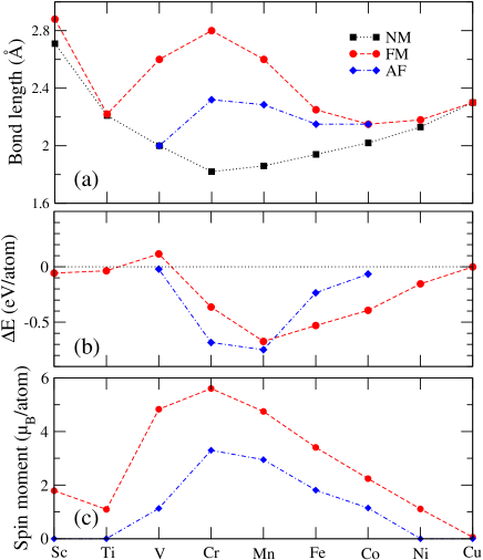
Figure 2: (color online) (a) Equilibrium bond lengths, (b) magnetization energy ($\Delta E$) (i.e., the total energy of a magnetic state relative to that of nonmagnetic state) ($\Delta E=E^{FM(AF)}-E^{NM}$) and (c) spin magnetic moments ($\mu_{B}$) of all the 3$d$ transition metal linear atomic chains in the NM, FM, and AF states.

III.1 Bond length and spin magnetic moment

The calculated equilibrium bond lengths ($d$) and atomic spin magnetic moments of all the 3$d$ transition metal linear chains in the NM, FM and AF states are displayed in Fig. 2 and also listed in Table I. The calculated total energy relative to that of the NM state (i.e., the magnetization energy) of the FM and AF linear atomic chains are also shown in Fig. 2 and Table I. It is clear from Fig. 2 that all the 3$d$ TM elements which are nonmagnetic in their bulk structures, become magnetic in the linear chain structures, though the FM Cu has a very small magnetic moment and is almost degenerate with the NM state (Table I). Furthermore, for all the 3$d$ TM elements, the NM state is metastable and the ground state is either FM and AF (see Fig. 2 and Table I). The V linear chain appears to be unique in that it has a large FM magnetic moment of 4.8 $\mu_{B}$/atom but its FM state is higher in energy than the NM state (Table I and Fig. 2b). Interestingly, Fig. 2 also shows that in all the cases, the equilibrium bond length is larger in a magnetic state than in the NM state. This is due to the larger kinetic energy in a magnetic state which make magnetic materials softer and larger in size. This magnetism induced increase in the bond length (or magneto-lattice expansion) can be as large as 54 %, as in the case of the Cr linear chain. The ground states for the Sc, Ti, Fe, Co, and Ni chains are ferromagnetic while that for the V, Cr and Mn chains are antiferromagnetic.

Table 1: Calculated equilibrium bond lengths ($d$) (in Å), total energies ($E_{t}$) (in eV/atom) in the FM and AF states (relative to the NM state), and spin magnetic moments ($m_{s}$) (in $\mu_{B}$/atom), of the 3$d$ transition metal linear chains.

	$d_{NM}$	$E_{t}^{FM}$	$m_{s}^{FM}$	$d_{FM}$	$E_{t}^{AF}$	$m_{s}^{AF}$	$d_{AF}$
Sc	2.71	-0.057	1.79	2.88	-	-	-
Ti	2.21	-0.036	0.77	2.22	-	-	-
V	2.00	0.116	4.06	2.60	-0.021	1.13	2.05
Cr	1.82	-0.363	5.60	2.80	-0.683	3.30	2.32
Mn	1.86	-0.673	4.75	2.60	-0.748	2.95	2.29
Fe	1.94	-0.530	3.41	2.25	-0.235	1.82	2.15
Co	2.02	-0.393	2.24	2.15	-0.066	1.15	2.15
Ni	2.13	-0.153	1.11	2.18	-	-	-
Cu	2.30	-0.001	0.06	2.30	-	-	-

The ground state bond lengths for the Sc, Ti, V, Cr, Mn, Fe, Co, Ni and Cu chains are 2.88, 2.22, 2.05, 2.32, 2.29, 2.25, 2.15, 2.18, 2.30 Å, respectively. These bond lengths are generally shorter than their counter-parts in the bulk structures. For example, the calculated bond lengths for AF bcc Cr, FM bcc Fe, FM fcc Co and FM fcc Ni are 2.43, 2.45, 2.48 and 2.49 Å, respectively. The chemical bonding environment in a wire is not the same as that in a bulk structure. In particular, the coordination number in a linear wire is certainly lower than in a bulk material, and this may result in a shorter bond length. Our predictions of the FM ground state for the Fe, Co, Ni and Cu are in good agreements with Refs. nau04, ; Spisak2, ; Bahn, ; Nautiyal2, . Our calculated bond lengths of the 3d TM linear chains in the FM state (Table I) agree well with many previous calculations. For example, previous theoretical bond lengths reported for the Fe, Ni and Co chains are 2.28 Ånau04 , and 2.25 ÅSpisak2 (Fe); 2.18 Ånau04 (Co); 2.18 Ånau04 , and 2.16 ÅBahn (Ni); 2.33 ÅBahn , and 2.29 ÅNautiyal2 (Cu). Our predictions of the AF ground state for the Cr and Mn linear chains are also consistent with the previous reports mok07 . Nonetheless, the energy difference between the FM and AF states in the Fe chain being 0.29 eV/atom, is somewhat smaller than previous results.Jisang2

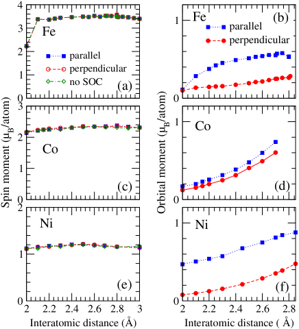
Figure 3: (color online) Spin (left panels) and orbital (right panels) magnetic moments as a function of interatomic distance of the ferromagnetic Fe, Co, and Ni linear atomic chains. ”Parallel” and ”perpendicular” denote the results from fully relativistic calculations with the magnetization parallel and perpendicular to the chain axis, respectively. In the left panels, ”no SOC” denote the results of the scalar relativistic calculations.

III.2 Spin-orbit coupling and orbital magnetic moment

The relativistic SOC is essential for the orbital magnetization and magnetocrystalline anisotropy in solids, though it may be weak in the 3$d$ transition metal systems. Therefore, unlike several previous studies of the magnetic properties of the 3$d$ TM chains, nau04 ; Spisak2 ; mok07 we include the SOC in our self-consistent calculations. When the SOC is taken into account, the spin moments for the linear atomic chains become 1.79 $\mu_{B}$ (Sc), 0.76 $\mu_{B}$ (Ti), 4.06 $\mu_{B}$ (V), 5.65 $\mu_{B}$ (Cr), 4.74 $\mu_{B}$ (Mn), 3.41 $\mu_{B}$ (Fe), 2.21 $\mu_{B}$ (Co), 1.17 $\mu_{B}$ (Ni), 0.08 $\mu_{B}$ (Cu), respectively. These values are almost identical to the corresponding ones obtained without the SOC (see also Fig. 3). This is due to the weakness of the SOC in the 3$d$ transition metals. However, including the SOC does give rise to a significant orbital magnetic moment in some atomic chains and, importantly, allows us to determine the easy magnetization axis in these 3$d$ atomic chains. For the magnetization along the chain direction, the calculated orbital magnetic moments in the FM state are 0.42, 0.23 and 0.45 $\mu_{B}$/atom for the Fe, Co and Ni chains, respectively, though they are only -0.04, -0.02, -0.16, -0.02, 0.04, and 0.0 $\mu_{B}$/atom for the Sc, Ti, V, Cr, Mn and Cu chains, respectively. The orbital moments in the Fe, Co and Ni atomic chains are, therefore, considerably enhanced, when compared with the bulk materials guo97 , and are also larger than the orbital moments in the Fe, Co, and Ni monolayers Guo ; Guo2

To see how the magnetic properties of the atomic chain evolve with the interatomic distance, we plot the spin and orbital moments for the Fe, Co, and Ni chains in the FM state as a function of the bond length in Fig. 3. For all three 3$d$ TM chains, the spin moment remains almost unchanged as the bond length is increased (Fig. 3). As mentioned before, the spin moment is also unaffected when the SOC is taken into account, due to the weakness of the SOC in 3$d$ transition metals. The same result is found even in the 4$d$ Mokrousov2 ; Delin2 ; Delin3 ; Simone and 5$d$ Delin TM linear atomic chains. Nonetheless, the SOC gives rise to rather pronounced orbital moments in all three cases, and these orbital moments increases significantly with the bond length, as can be seen in Fig. 3. Significantly, the orbital moment shows a strong dependence on the magnetization orientation (Fig. 3). The orbital moment for the magnetization along the chain is higher than that for the magnetization perpendicular to the chain. The orbital moments of the Fe, Co, and Ni chains at its equilibrium bond length with a perpendicular magnetization are only 0.15, 0.17, and 0.12 $\mu_{B}$, respectively. This anisotropy in the orbital moment is especially pronounced in the Ni chain. It is well known that in general, the magnetization direction with a larger orbital moment, would be lower in total energy. Therefore, the easy magnetization direction in the Fe, Co, and Ni chains is expected to be along the chain, as will be reported in Sec. V. Finally, we notice that our results for the spin and orbital moments are in good agreement with previous calculations for the FeMokrousov2 ; aut06 and CoLazarovits linear chains.

III.3 Band structure and density of states

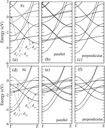
Figure 4: Band structures of the Fe (upper panels) and Ni (lower panels) linear chains at the equilibrium bond length. Left panels: the scalar-relativistic band structures; the middle and right panels: the fully relativistic band structures with the the magnetization parallel to and perpendicular to the chain axis, respectively. In the left panels, the solid and dashed lines represent (spin up) and (spin down) bands, respectively. The Fermi level (the dotted horizontal line) is at the zero energy.

In order to understand the calculated magnetic properties, let us now examine the band structure of the 3$d$ transition metal linear chains. Ploted in Fig. 4 is the band structure obtained without and also with the SOC for the Fe and Ni linear chains in the FM state at the equilibrium interatomic distance. In the absence of the SOC, because of the linear chain symmetry, the bands may be grouped into three sets, namely, the nondegenerate $s$- and $d_{z^{2}}$-dominant bands, double degenerate (d_xz, d_yz), and (d${}_{x^{2}-y^{2}}$, d_xy) dominant bands (see the left panels in Fig. 4). The (d${}_{x^{2}-y^{2}}$, d_xy) bands are narrow because the $d_{x^{2}-y^{2}}$ and $d_{xy}$ orbitals are perpendicular to the chain, thus forming weak $\delta$ bonds. The (d_xz, d_yz) bands, on the other hands, are more dispersive due to the stronger overlap of the $d_{xz}$ and $d_{yz}$ orbitals along the chain, which gives rise to the $\pi$ bonds. The $s$- and $d_{z^{2}}$ dominant bands are most dispersive since these orbitals form strong $\sigma$ bonds along the chain. In the FM state, these bands are exchange split, and this splitting into the spin-up and spin-down bands is 0.64, 2.58, 3.44, 3.67, 2.99, 1.94, 0.96, and 0.04 eV for the Sc, Ti, V, Cr, Mn, Fe, Co, Ni and Cu chains. The size of this spin-splitting could be correlated with the spin moment in the FM state (see Table I). Also, Fig. 4 shows that when the band filling increases, as one moves from Fe to Ni, the (d${}_{x^{2}-y^{2}}$, d_xy) bands which are partially occupied in the Fe chain, now lie completely below the Fermi level in the Ni chain, and hence play no role in magnetism.

The directional dependence of the magnetization can be explained by analyzing the fully relativistic band structures (see Fig. 4). For the Fe linear chain with the axial magnetization (Fig. 4b), the doubly degenerate d${}_{x^{2}-y^{2}}$, d_xy bands are split into two with angular momenta $m_{l}$= $\pm$2. If one of them is fully occupied and the other is empty, the resulting orbital moment is 2. Nonetheless, in the Fe linear chain, both are partially occupied with different occupation numbers (Fig. 4b), resulting in an orbital moment of 0.42 $\mu_{B}$/atom. Of course, the larger the SOC splitting, the larger the difference in the occupation number and hence the larger the orbital moment. However, for the perpendicular magnetization, the d${}_{x^{2}-y^{2}}$, d_xy bands remain degenerate (Fig. 4c) and hence do not contribute to orbital magnetization. Therefore, the Fe linear chain would have a smaller orbital magnetic moment. Of course, when the SOC is included, the degenerate d_xz, d_yz bands are also split into the $m_{l}=-1$ and +1 bands for the axial magnetization, but remain degenerate for the perpendicular magnetization (see Fig. 4). This SOC splitting of the ($d_{xz}$, $d_{yz}$) band and ($d_{x^{2}-y^{2}}$, $d_{xy}$) band is proportional to $|<d_{xz}|H_{SO}|d_{yz}>|^{2}$ and $|<d_{x^{2}-y^{2}}|H_{SO}|d_{xy}>|^{2}$, respectively. Here $H_{SO}$ is the SOC Hamiltonian. Since $|<d_{xz}|H_{SO}|d_{yz}>|^{2}$:$|<d_{x^{2}-y^{2}}|H_{SO}|d_{xy}>|^{2}$ = 1:4, tak76 the SOC splitting of the ($d_{xz}$, $d_{yz}$) bands is much smaller than the ($d_{x^{2}-y^{2}}$, $d_{xy}$) bands (see Figs. 4-5). Therefore, the ($d_{xz}$, $d_{yz}$) bands would make a much smaller contribution to the orbital magnetization and also the magnetocrystalline anisotropy which will be discussed in Sec. V.

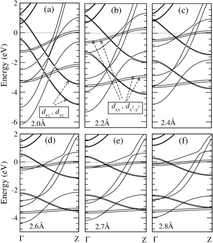
Figure 5: Band structures of the Fe linear chain with the magnetization along the chain axis at several interatomic distances. The Fermi level (the dotted horizontal line) is the zero energy.

In Fig. 5, the band structure of the Fe linear chain at several different interatomic distances with the magnetization along the chain direction is displayed. Fig. 3b shows that the Fe orbital moment for both magnetization orientations increases with the interatomic distance. However, the increase for the magnetization along the chain axis is much more dramatic than for the perpendicular magnetization. The reason for this variation of the orbital moment with the interatomic distance is two fold. One is due to the increase in the localization of the 3$d$ orbital wave function with the interatomic distance. The other is due to the detailed change in the band structure. For example, as the interatomic distance goes from 2.4 Å (Fig. 5c) to 2.6 Å (Fig. 5d), one of the SOC split (d${}_{x^{2}-y^{2}}$, d_xy) bands becomes fully occupied, resulting in the increase in the occupation number difference in the two $m_{l}$= $\pm$2 bands and hence in a larger orbital moment.

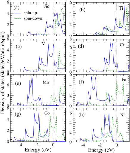
Figure 6: (color online) Density of states of the FM 3d TM linear atomic chains at the equilibrium bond length. The Fermi level (dotted vertical lines) is at the zero energy.

Electric and spin current transports are determined by the characteristics of the band structure near the Fermi level ($E_{F}$) in the systems concerned. Therefore, it would be interesting to examine the energy bands and density of states (DOS) of the atomic chains in the vicinity of the $E_{F}$. The spin-decomposed DOS for the FM Sc, V, Cr, Mn, Fe, Co, Ni linear chains are displayed in Fig. 6. In the Fe, Co, Ni cases, the spin-up states are nearly completely filled, and hence, the DOS at the $E_{F}$ is low. On the other hand, the spin-down states are only partially occupied, resulting in a large DOS at the $E_{F}$. Therefore, the density of states at the $E_{F}$ in these systems are highly spin-polarized. This is usually quantified by the spin-polarization $P$ defined as

$$P=\frac{N_{\uparrow}(E_{F})-N_{\downarrow}(E_{F})}{N_{\uparrow}(E_{F})+N_{\downarrow}(E_{F})},$$ (1)

where $N_{\uparrow}(E_{F})$ and $N_{\downarrow}(E_{F})$ are the spin-up and spin-down DOS at the $E_{F}$, respectively. The most useful materials for the spintronic applications are the so-called half-metallic materials in which one spin channel is metallic and the other spin channel is insulating. The spin-polarization for these half-metals is either 1.0 or -1.0, and the electric conduction would be fully spin-polarized. The calculated spin-polarization and also the numbers of the conduction bands that cross the Fermi level in the 3$d$ TM chains are listed in Table II. It is clear that the FM V, Fe, Co, Ni linear chains have a very high spin-polarization, though none of the 3$d$ TM linear chains in the FM state is half-metallic. Our calculated spin-polarization for the bulk FM bcc Fe, fcc Co, and fcc Ni is -0.55, -0.77, -0.81, respectively, being considerably smaller than the spin-polarization of the corresponding linear chains. This suggests that the Sc, V, Mn, Fe, Co, and Ni nanowires may be good potential materials for spintronic devices. wol01 Interestingly, the FM V chain has a large positive spin polarization (Table II and Fig. 6).

Table 2: Numbers ($n_{c}^{\uparrow}$ and $n_{c}^{\downarrow}$) of the spin-up and spin-down conduction bands crossing the Fermi level, and spin-polarization $P$ at the Fermi level in the 3$d$ TM atomic chains in the FM state. The spin-polarization $P$ for the bulk FM bcc Fe, fcc Co and fcc Ni are -0.55, -0.77 and -0.81, respectively

	linear chain		zigzag chain
	($n^{\uparrow}_{c}$, $n^{\downarrow}_{c}$)	$P$	($n^{\uparrow}_{c}$, $n^{\downarrow}_{c}$)	$P$
Sc	(4, 1)	0.881	(3, 0)	0.610
Ti	(5, 4)	0.416	(4, 4)	0.181
V	(6, 1)	0.930	(3, 3)	0.085
Cr	(3, 1)	0.777	(4, 2)	0.481
Mn	(1, 3)	-0.869	(2, 1)	-0.829
Fe	(1, 6)	-0.961	(2, 4)	-0.643
Co	(1, 6)	-0.920	(2, 7)	-0.884
Ni	(1, 6)	-0.951	(2, 2)	-0.890

The magnetic properties and spin-polarization near the Fermi level in the linear Fe, Co and Ni chains have been calculated from ab initio before by several groups.Jisang ; nau04 ; aut06 In particular, the free-standing FM Fe, Co and Ni linear chains are reported to be nearly half-metallic in Ref. nau04, , being in agreement with our findings (Table II). Experimentally, a clear peak at 0.5 $G_{0}$ ($G_{0}=2e^{2}/h$ being the conductance quantum) was observed recently in the conductance of the Co chainRodrigues , indicating a fully polarized conduction in this monoatomic chain system.

IV Zigzag chains

The zigzag structure for monoatomic wires has already been observed in experiments whi91 , and also proposed in theoretical calculationsSpisak2 ; Ribeiro ; li05 ; Portal1 . However, among 3$d$ transition metals, only the Ti and Fe zigzag chains have been studied theoretically Spisak2 ; li05 . In the present paper, we perform a systematic ab initio study of the structural, electronic and magnetic properties of the zigzag chain structure of all the 3$d$ transition metals.

Table 3: Equilibrium structural parameters (see Fig. 1b for symbols $d_{1}$, $d_{2}$, $\alpha$), spin magnetic moment ($m_{s}$) and magnetization energy ($\Delta E$) (i.e., the total energy of a magnetic state relative to that of the NM state) of the 3$d$ transition metal zigzag chains. $d_{1}$ and $d_{2}$ are in the unit of Å, and $\alpha$ is in the unit of degree. $\Delta E$ is in the unit of eV/atom, and $m_{s}$ in the unit of $\mu_{B}$/atom.

State		Sc	Ti	V	Cr	Mn	Fe	Co	Ni	Cu
	$d_{1}$	2.911	2.718	2.627	2.213	2.264	2.271	2.258	2.067	2.371
NM	$d_{2}$	2.910	2.364	2.067	2.162	2.079	2.095	2.228	3.275	2.334
	$\alpha$	60.01	54.91	50.55	59.23	57.02	57.18	59.56	71.60	59.56
	$d_{1}$	2.910	2.720	2.626	2.831	2.700	2.429	2.318	2.288	-
	$d_{2}$	2.938	2.366	2.066	2.766	2.480	2.240	2.218	2.275	-
FM	$\alpha$	59.68	54.91	50.55	59.23	57.02	57.18	58.50	59.82	-
	$m_{s}$	1.050	0.571	0.027	5.904	4.368	3.006	2.049	0.867	-
	$\Delta E$	-0.527	0.002	0.000	0.049	-0.574	-0.779	-0.485	-0.714	-
	$d_{1}$	-	-	-	2.587	2.628	2.179	2.313	2.262	-
	$d_{2}$	-	-	-	2.531	2.413	3.765	2.213	2.301	-
AF	$\alpha$	-	-	-	59.27	57.00	73.18	58.50	60.55	-
	$m_{s}$	-	-	-	3.478	3.208	3.062	1.311	0.563	-
	$\Delta E$	-	-	-	-0.336	-0.565	0.098	-0.139	-0.647	-

IV.1 Structure and magnetic moment

The calculated equilibrium structural parameters (Fig. 1), spin magnetic moment and magnetization energy of the 3$d$ TM zigzag chains are listed in Table III. First of all, the bond length between two nearest ions ($d_{2}$) in the zigzag chains is generally similar to that ($d$) of the corresponding linear chains, though the distance ($d_{1}$) between two ions in the zigzag chains along the chain direction (z axis) is somewhat larger than the linear chains (see Table III). Interestingly, most of the zigzag chains are like planar equilateral triangle ribbens (Fig. 1b) except the AF Fe and NM Ni zigzag chains which look more like a sheared two-leg ladder ($\alpha\geq 71^{\circ}$, $d_{1}<d_{2}$; see Table III). Note that the calculated structural parameters ($d_{1}$, $d_{2}$, $\alpha$ in Table III) of the NM Ti zigzag chain are similar to that ($d_{1}=2.58$ Å, $d_{2}=2.41$ Å, $\alpha=57.6$) reported previously in Ref. li05, . For a FM state of the Fe zigzag chain, $\alpha=56$ and $m_{s}=2.9\mu_{B}$ were reported in Ref. Spisak2, , being close to the corresponding values listed in Table III here.

Secondly, all the 3$d$ TM zigzag chains except that of Cu, have magnetic solutions. Furthermore, one can see that the Sc, Mn, Fe, Co, and Ni zigzag chains are most stable in the FM state, whilst the ground state of the Ti and V chains is the NM state and that of the Cr chain is the AF state. Note that the ground state of the linear Ti (V, Mn) chain is the FM (AF) state (Table I). Thirdly, the spin magnetic moments in the zigzag chains (Table III) are generally smaller than in the corresponding linear chains (Table I). This is due to the increase in the coordination number in the zigzag chains because most of them form a planar equilateral triangle ribben. Note that our calculated spin magnetic moments for the bulk FM Fe, Co and Ni are 2.19, 1.60 and 0.63 $\mu_{B}$/atom, respectively, being considerably smaller than both the linear and zigzag chains. Nonetheless, as for the linear chains, the Cr zigzag chain still has the largest spin magnetic moment (Table III).

When the SOC is taken into account, the spin magnetic moments of the zigzag chains remain almost unchanged, as for the linear chain cases. The orbital magnetic moments of the FM zigzag chains with the magnetization along the $z$-axis are -0.003 (Sc), -0.005 (Ti), 0.000 (V), 0.000 (Cr), 0.025 (Mn), 0.087 (Fe), 0.149 (Co), and 0.096 (Ni) $\mu_{B}$/atom, being significantly smaller than that of the corresponding linear chains (see Sec. IIIb).

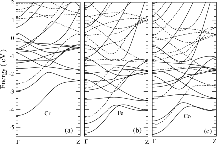
Figure 7: Scalar-relativistic band structures of the Cr, Fe, and Co zigzag atomic chains in the FM state. The Fermi level (the dotted horizontal line) is at the zero energy.

IV.2 Band structures and density of states

The scalar-relativistic band structures of the FM Cr, Fe and Co zigzag chains are displayed in Fig. 7, as representatives. Compared with the corresponding band structures of the linear chains (Fig. 4a), the number of bands become doubled in the zigzag chains because of the doubling of the number of atoms. Furthermore, unlike the linear chains where the $d_{xy}(d_{xz})$ and $d_{x^{2}-y^{2}}(d_{yz})$ bands (Fig. 4a and 4d) are degenerate because of rotational invariance, the $d_{xy}(d_{xz})$ and $d_{x^{2}-y^{2}}(d_{yz})$ bands are now split because of the strong anisotropy in the $x-y$ plane perpendicular to the chain axis. It is clear that the energy bands are also highly spin-split and the separation of the spin-up and spin-down bands may be correlated with the spin magnetic moment. For example, the spin-splitting of the lowest bands is 1.78 eV in the Cr chain, but is only 0.89 and 0.50 eV for the Fe and Co chains, respectively.

As for the linear chains, we calculate the spin-polarization ($P$) and count the numbers of spin-up and spin-down conduction bands at the Fermi level in the FM zigzag chains, as listed in Table II. Nevertheless, the $P$ in the V, Mn, Fe, Co and Ni zigzag chains all gets reduced (Table II). The largest reduction is the V zigzag chain, being reduced from 0.939 to 0.085. The reduction is small for the Mn, Co and Ni chains (Table II), suggesting that the FM Mn, Co and Ni zigzag chains are still useful for spintronic applications.

IV.3 Stability of linear chain structures

Let us now compare the total energies of the linear and zigzag chains and examine the relative stability of the two structures. The ground state cohesive energy of the linear chains and the cohesive energies of the zigzag chains in the NM, FM and AF states are displayed in Fig. 8. The cohesive energy ($E_{c}$) of an atomic chain is defined as the difference between the sum of the total energy of the free constituent atoms ($E_{a}$) and the total energy of the chain ($E_{t}$), i.e. $E_{c}=E_{a}-E_{t}$. A positive value of the $E_{c}$ means that the formation of the chain from the free atoms would save energy, i.e., the chain would be stable against breaking up into free atoms. The total energies of the free atoms are calculated by the cubic box supercell approach with the cell size of 10 Å. The electronic configurations used are $3d^{1}4s^{2}$ (Sc), $3d^{3}4s^{1}$ (Ti), $3d^{4}4s^{1}$ (V), $3d^{5}4s^{1}$ (Cr), $3d^{6}4s^{1}$ (Mn), $3d^{7}4s^{1}$ (Fe), $3d^{8}4s^{1}$ (Co), $3d^{9}4s^{1}$ (Ni) and $3d^{10}4s^{1}$ (Cu).

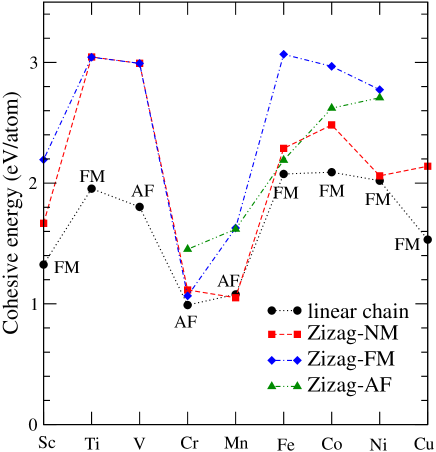
Figure 8: (color online) The cohesive energy of the 3$d$ TM zigzag chains in the NM, FM and AF states. For comparison, the ground state cohesive energy of the corresponding linear chains is also plotted (solid circles). The ground state magnetic configuration of the linear chains is labelled as NM or FM or AF near each solid circle.

Remarkably, Fig. 8 shows that in all the cases, the ground state cohesive energy of the linear chain is smaller than that of the zigzag chain in a magnetic state. This suggests that the 3$d$ linear chains are unstable against the zigzag structural distortion, as may be expected from the Peierls instability of linear one-dimensional monoatomic metals. kit96 The difference in the ground state energy between the linear and zigzag structures for all the 3$d$ elements is rather large, ranging from 0.8 to 1.1 eV/atom. This shows that the free standing 3$d$ TM linear chains would not be the stable state, and the linear chains may occur only in constrained conditions such as on the steps on a vicinal surface Gambardella2 and under tensile stress in the break-point experiments Rodrigues ; Rodrigues2 ; Jiandong ; Susumu ; Ohnishi . Only the zigzag structure of Fe has been considered before in Ref.  Spisak2, . The zigzag structure of Fe was also found to be lower in energy than the linear chain by 1.01 eV/atom, a value being close to 0.99 eV/atom found in the present calculations.

Interestingly, we find that for some 3$d$ transition metals, the ground state magnetic configuration changes when the structure changes from the linear to zigzag chain. For example, the ground state of the Sc and Ti chains is ferromagnetic in the linear chain but becomes nonmagnetic in the zigzag structure (Table III). On the other hand, the ground state of the Mn chain changes from the AF in the linear chain to the FM state in the zigzag structure. Nevertheless, the total energy difference between the FM and AF states in the Mn zigzag chain is small (within $\sim$0.01 eV/atom). The ground state of the V chain also changes, from the AF state in the linear chain to the FM state in the zigzag chain.

V Magnetic anisotropy energy

The total energy as a function of the magnetization orientation ($\theta,\phi$) of a 1D wire may be written, in the lowest non-vanishing terms, as

$$E_{t}=E_{0}+sin^{2}\theta(E_{1}-E_{2}cos^{2}\phi)$$ (2)

where $\theta$ is the polar angle of the magnetization away from the chain axis ($z$-axis) and $\phi$ is the azimuthal angle in the $x-y$ plane perpendicular to the wire, measured from the x axis. For the free standing linear atomic chains, the azimuthal anisotropy energy constant $E_{2}$ is zero, because of the rotational invariance. The axial anisotropy energy constant $E_{1}$ is then given by the total energy difference between the magnetization along the $y$($x$) and z axes, i.e., $E_{1}=E^{y}-E^{z}$ ($E^{x}=E^{y}$). A positive value of $E_{1}$ means that the chain ($z$) axis is the easy magnetization axis. For the zigzag chains which are in the $x-z$ plane, $E_{2}$ is not zero and can be calculated as the total energy difference between the magnetization along the $x$ and $y$ axes, i.e., $E_{2}=E^{y}-E^{x}$.

Table 4: Total ($E_{1}^{t}$), electronic ($E_{1}^{e}$) and dipolar ($E_{1}^{d}$) magnetic anisotropy energes (in meV/atom) of the 3$d$ transition metal linear chains. If $E_{1}^{t}$ is positive, the easy magnetization axis is along the chain; otherwise, the easy magnetization axis is perpendicular to the chain.

	FM			AF
	$E_{1}^{t}$	$E_{1}^{e}$	$E_{1}^{d}$	$E_{1}^{t}$	$E_{1}^{e}$	$E_{1}^{d}$
Sc	0.06	0.01	0.05	-	-	-
Ti	-0.22	-0.27	0.05	-	-	-
V	0.81	0.45	0.36	0.183	0.138	0.045
Cr	0.62	0.07	0.55	-0.006	-0.259	0.253
Mn	0.22	-0.28	0.50	-0.487	-0.698	0.212
Fe	2.65	2.25	0.40	-0.817	-0.917	0.100
Co	-0.48	-0.68	0.20	5.194	5.155	0.039
Ni	11.44	11.39	0.05	-	-	-

The magnetic anisotropy energy for a magnetic solid consists of two contributions. One comes from the magnetocrystalline anisotropy in the electronic band structure caused by the simultaneous occurrence of the electron spin-orbit interaction and spin-polarization in the magnetic system. This is known as the electronic contribution and ab initio calculation of this part has already been described in Sec. II. The other is the magnetostatic (or shape) anisotropy energy due to the magnetic dipolar interaction in the solid. The shape anisotropy energy is zero for the cubic systems such as bcc Fe and fcc Ni, and also negligibly small for weakly anisotropic solids such as hcp Co. However, for the highly anisotropic structures such as magnetic Fe and Co monolayers, Guo ; Guo2 the shape anisotropy energy can be comparable to the electronic MAE, and therefore cannot be be neglected. Furthermore, as will be reported immediately below, the shape anisotropy energy of the 3$d$ TM atomic chains are also large and cannot be ignored. Therefore, in this work, following Ref. Guo, , we use Ewald’s lattice summation techniqueEwald to calculate the magnetic dipole-dipole interaction energy. For the collinear magnetic systems (i.e. m_q//m${}_{q^{{}^{\prime}}}$), this magnetic dipolar energy $E_{d}$ is given by (in atomic Rydberg units) Guo

$$E^{d}=\sum_{qq^{{}^{\prime}}}{\frac{m_{q}m_{q^{{}^{\prime}}}}{c^{2}}M_{qq^{{}^{\prime}}}}$$ (3)

and

$$M_{qq^{{}^{\prime}}}={\sum_{\bf R}}^{{}^{\prime}}\frac{1}{\mid\bf R+q+q^{{}^{\prime}}\mid^{3}}\{1-3\frac{[(\bf R+q+q^{{}^{\prime}})\cdot\hat{m_{q}}]^{2}}{\mid\bf R+q+q^{{}^{\prime}}\mid^{2}}\}$$ (4)

where $M_{qq^{{}^{\prime}}}$ is called the magnetic dipolar Madelung constant which is evaluated by Ewald’s lattice summation technique Ewald . The speed of light $c=274.072$. R are the lattice vectors, q are the atomic position vectors in the unit cell and $m_{q}$ is the atomic magnetic moment on site q. Note that in atomic Rydberg units, one Bohr magneton ($\mu_{B}$) is $\sqrt{2}$. Therefore, the magnetic dipolar energy $E^{d}$ for the multilayers obtained previously by Guo and co-workersGuo ; Guo2 ; guo92 ; guo94 ; guo99 is too small by a factor of $2$.

Table 5: The total ($E_{1}^{t}$, $E_{2}^{t}$), electronic ($E_{1}^{e}$, $E_{2}^{e}$) and dipolar ($E_{1}^{d}$, $E_{2}^{d}$) magnetic anisotropy energy constants (in meV/atom) as well as the easy magnetization axis (M) of the 3$d$ transition metal zigzag chains. $E_{1}$ = $E^{y}$ - $E^{z}$; $E_{2}$ = $E^{y}$ - $E^{x}$, see Eq. (2).

	FM					AF
	$E_{1}^{e}$	$E_{2}^{e}$	$E_{1}^{d}$	$E_{2}^{d}$	$E_{1}^{t}$	$E_{2}^{t}$	M	$E_{1}^{e}$	$E_{2}^{e}$	$E_{1}^{d}$	$E_{2}^{d}$	$E_{1}^{t}$	$E_{2}^{t}$	M
Sc	0.000	0.000	0.022	0.011	0.022	0.011	$z$	-	-	-	-	-	-	-
Ti	0.000	0.000	0.010	0.006	0.010	0.006	$z$	-	-	-	-	-	-	-
V	0.000	0.000	0.000	0.000	0.000	0.000	-	-	-	-	-	-	-	-
Cr	-0.158	-0.158	0.857	0.418	0.699	0.260	$z$	-2.663	-2.754	0.152	-0.190	-2.511	-2.944	$y$
Mn	-0.194	-0.256	0.578	0.299	0.384	0.043	$z$	0.898	1.024	0.091	-0.190	0.989	0.834	$z$
Fe	-0.700	-0.584	0.374	0.193	-0.326	-0.391	$y$	0.012	0.006	0.315	-0.071	0.327	-0.065	$z$
Co	1.317	1.122	0.192	0.096	1.509	1.218	$z$	8.763	6.992	0.029	-0.040	8.792	6.952	$z$
Ni	0.636	1.741	0.035	0.017	0.671	1.758	$x$	6.911	5.126	0.006	-0.007	6.917	5.119	$z$

The calculated shape anisotropy energies ($E^{d}$) for the linear and zigzag chains are listed in Tables IV and V, respectively. Tables IV and V show that in both the linear and zigzag chains and in both the FM and AF states, the shape anisotropy energies can be comparable to the electronic contributions. Furthermore, they always prefer the chain direction ($z$ axis) as the easy magnetization axis, and this may be expected since the shape anisotropy energy always favors the direction of the longest dimension. Therefore, any perpendicular magnetic anisotropy must originate from the electronic magnetocrystalline anisotropy when it overcomes the shape anisotropy. In the zigzag chains, there is also a significant magnetic anisotropy in the $x-y$ plane perpendicular to the chain axis. For the FM state, the $x$ axis is favored in all the zigzag chains, i.e., the $y$ axis would be the hard magnetization axis if the magnetic anisotropy were determined by the $E^{d}$ alone. In contrast, for the AF state, the $x$ axis would be the hard axis (see Table V).

The calculated electronic anisotropy energies of the linear and zigzag atomic chains are also listed in Tables IV and V, respectively. Interestingly, Table IV shows that in the FM linear chains, the electronic anisotropy energy would favor a perpendicular anisotropy in the Ti, Mn, Co chains but prefer the chain axis in the Sc, V, Cr, Fe and Ni chains. Nevertheless, the easy magnetization direction is predicted to be the chain axis in all the 3$d$ FM linear chains except Ti and Co because the perpendicular electronic anisotropy in the Mn chain is not sufficiently large to overcome the axial shape anisotropy (Table IV). In the AF state, in contrast, the Cr, Mn and Fe linear chains would have the easy axis perpendicular to the chain while the V and Co linear chains still prefer the axial anisotropy. Remarkably, the FM Ni linear chain has a gigantic axial anisotropy energy (Table IV), being in the same order of magnitude of that in the 4$d$ transition metal linear chains Mokrousov . In the 4$d$ transition metals, the SOC splittings are large, being about ten times larger than the 3$d$ transition metals, and thus the large MAE in the 4$d$ transition metal linear chains may be expected. The axial anisotropy energy for the FM V, Cr, Fe and AF Co linear chains are also rather large, being generally a few times larger than the corresponding monolayers. Guo ; Guo2

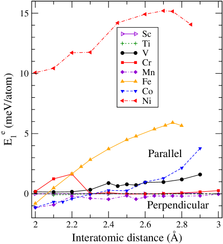
Figure 9: (color online) Magnetocrystalline anisotropy energy ($E_{1}^{e}$) of the 3$d$ transition metal linear atomic chain as a function of interatomic distance. A positive value of $E_{1}^{e}$ means that the magnetization would be parallel to the chain axis whilst a negative value would means that the easy magnetization axis would be perpendicular to the chain.

In Fig. 9, the electronic anisotropy energy for the linear 3$d$ atomic chains is displayed as a function of the lattice constant (bond length). It is clear that in all the 3$d$ linear chains except that of Fe and Co, the easy axis of magnetization remains the same no matter the chain is elongated or compressed. When compressed, the FM Fe linear chain would undergo a spin reorientation transition from the axial to perpendicular direction at the bondlength of $\sim$2.06Å. In contrast, the FM Co linear chain would transform from the perpendicular to axial direction at $\sim$2.31 Å when elongated.

To help identifying the electronic origin of the magnetocrystalline anisotropy, we plot the scalar-relativistic $d$-orbital decomposed DOS for the FM Fe, Co and Ni linear chains in Fig. 10. According to perturbation theory analysis, the occupied and empty $d$-states in the vicinity of the Fermi level which are coupled by the SOC are most important to the magnetocrystalline anisotropy wan93 . Furthermore, the SOC matrix elements $<d_{xz}|H_{SO}|d_{yz}>$ and $<d_{x^{2}-y^{2}}|H_{SO}|d_{xy}>$ are found to contribute to the axial anisotropy while $<d_{x^{2}-y^{2}}|H_{SO}|d_{yz}>$, $<d_{xy}|H_{SO}|d_{xz}>$ and $<d_{3z^{2}-r^{2}}|H_{SO}|d_{yz}>$ prefer a perpendicular anisotropy. tak76 The ratio of these matrix elements are $<d_{xz}|H_{SO}|d_{yz}>^{2}$:$<d_{x^{2}-y^{2}}|H_{SO}|d_{xy}>^{2}$: $<d_{x^{2}-y^{2}}|H_{SO}|d_{yz}>^{2}$:$<d_{xy}|H_{SO}|d_{xz}>^{2}$:$<d_{3z^{2}-r^{2}}|H_{SO}|d_{yz}>|^{2}$ =$1:4:1:1:3$. tak76 Fig. 10 (a,d) shows that in the FM Fe and Ni chains, the $E_{F}$ sits on, respectively, the lower and upper sharp peak of the spin-down $d_{x^{2}-y^{2}}$ and $d_{xy}$ DOS. Consequently, the SOC near the $E_{F}$ between the $d_{x^{2}-y^{2}}$ and $d_{xy}$ bands would give rise to a dominating contribution to the magnetocrystalline anisotropy and therefore, the FM Fe and Ni chains would prefer the chain axis. On the other hand, in the FM Co chain, the $E_{F}$ lies in the valley of the spin-down $d_{x^{2}-y^{2}}$ and $d_{xy}$ DOS (Fig. 10 b). As a result, the $<d_{x^{2}-y^{2}}|H_{SO}|d_{xy}>$ contribution does not dominate and the FM Co chain would perfer a perpendicular anisotropy. Nonetheless, the spin-down $d_{x^{2}-y^{2}}$ and $d_{xy}$ DOS near the $E_{F}$ increases dramatically when the FM Co chain is stretched (Fig. 10 c). This would enhance the $<d_{x^{2}-y^{2}}|H_{SO}|d_{xy}>$ contribution considerably and the FM Co chain would then prefer the axial anisotropy when the bondlength is larger than $\sim$2.23 Å (Fig. 9).

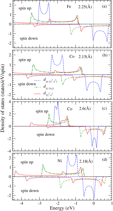
Figure 10: (color online) $d$-orbital-decomposed density of states of the FM (a) Fe, (b) Co and (d) Ni linear chains at the equilibrium bond length. In (c), $d$-orbital-decomposed density of states of the FM Co linear chain at an elongated bond length of 2.6 Å is displayed.

Generally speaking, the magnetic anisotropy in at least the FM 3$d$ chains becomes smaller as the structure moves from the linear to zigzag structure (see Tables IV and V). The most dramatic reduction in the magnetic anisotropy occurs in the FM Ni chain. The axial anisotropy constant $E_{1}$ in the zigzag Ni chain is one order of magnitude smaller than that in the linear chain. There is now a large anisotropy energy ($E_{2}$) in the $x-y$ plane perpendicular to the chain axis (see Table V). As a result, the easy magnetization axis in the zigzag FM Ni chain is in the zigzag chain plane but perpendicular to the chain axis, i.e., the $x$-axis (see Fig. 1). For the FM Ti and Co chains, the easy magnetization changes from the perpendicular to axial direction (Tables IV and V). Strikingly, no AF state could be stabilized in the linear Ni chain, and in contrast, the AF state not only can be stabilized but also has gigantic magnetic anisotropy energies in the zigzag chain (see Table V). Table V also shows that the magnetic anisotropy energies in the zigzag AF Co chain are considerably enhanced compared with that in the linear AF Co chain.

VI Conclusions

We have performed a systematic ab initio study of the magnetic and electronic properties of both linear and zigzag atomic chains of all 3$d$ transition metals within density functional theory with GGA. The accurate frozen-core full-potential PAW method is used. The underlying atomic structures were determined theoretically. All the zigzag chains except the NM Ni and AF Fe chains which form a twisted two-legger ladder, look like a corner-sharing triangle ribbon, and have a lower total energy than the corresponding linear chains.

We find that all the 3$d$ transition metals in both linear and zigzag structures have a stable or metastable FM state. Furthermore, in the V, Cr, Mn, Fe, Co linear chains and Cr, Mn, Fe, Co, Ni zigzag chains, a stable or metastable AF state exists too. In the Sc, Ti, Fe, Co, Ni linear structures, the FM state is the ground state whilst in the V, Cr and Mn linear chains, the AF state is most energetically favorable. The electronic spin-polarization at the Fermi level in the FM Sc, V, Mn, Fe, Co and Ni linear chains is close to 90% or above, suggesting that these nanostructures may have applications in spin-transport devices. Only in the Cr zigzag structure, the AF state is energetically more favorable than the FM state. Surprisingly, the V, Cr, Mn, and Fe linear chains show a giant magneto-lattice expansion of up to 54 %.

Both the electronic magnetocrystalline anisotropy energy and magnetic dipolar anisotropy energy have been calculated. We find that shape anisotropy energy can be comparable to the electronic one and always prefer the axial magnetization in both the linear and zigzag structures. Furthermore, in the zigzag chains, there is also a pronounced shape anisotropy in the plane perpendicular to the chain axis. Nonetheless, in the FM Ti, Mn, Co and AF Cr, Mn, Fe linear chains, the electronic anisotropy is perpendicular, and it is sufficiently large in the FM Ti and Co as well as the AF Cr, Mn and Fe linear chains such that the easy magnetization axis is perpendicular. In the AF Cr and FM Ni zigzag structures, the easy magnetization direction is also perpendicular to the chain axis but in the ribbon plane. Remarkably, the axial magnetic anisotropy in the FM Ni linear chain is gigantic, being $\sim$ 12 meV/atom, suggesting that Ni nanowires could have important applications in ultrahigh density magnetic memories and hard disks. The axial magnetic anisotropy energy of the FM V, Cr, Fe linear chains and FM Cr, Mn, Co zigzag structures is also sizable. Interestingly, there is a spin-reorientation transition in the FM Fe and Co linear chains when the chains are compressed or elongated. Large orbital magnetic moment is found in the FM Fe, Co and Ni linear chains. Finally, the electronic band structure and density of states of the nanowires have also been calculated mainly in order to understand the electronic origin of the large magnetocrystalline anisotropy and orbital magnetic moment.

References

- (1) S. Heinze, M. Bode, A. Kubetzka, O. Pietzsch, X. Nie, S. Blügel, and R. Wiesendanger, Science , 1805 (2000)
- (2) O. Pietzsch, A. Kubetzka, M. Bode, and R. Wiesendanger, Phys. Rev. Lett. , 5212 (2000)
- (3) A. Hernando, P. Crespo, M. A. Garcia, E. F. Pinel, J. de la Venta, A. Fernández, and S. Penadés, Phys. Rev.B , 052403 (2006).
- (4) A. Hernando, P. Crespo, and M. A. Garcia, Phys. Rev. Lett. , 057206 (2006).
- (5) N. D. Mermin and H. Wagner, Phys. Rev. Lett. , 1133-1136 (1966).
- (6) P. Gambardella, A. Dallmeyer, K. Maiti, M. C. Malagoli, W. Eberhardt, K. Kern C. Carbone, Nature , 301 (2002).
- (7) S. B. Suh, B. H. Hong, P. Tarakeshwar, S. J. Youn, S. Jeong, and K. S. Kim, Phys. Rev. B , 241402(R) (2003).
- (8) G. Rubio, N. Agrait, and S. Vieira, Phys. Rev. Lett. , 2302 (1996).
- (9) V. Rodrigues, J. Bettini, P. C. Silva and D. Ugarte, Phys. Rev. Lett. , 096801 (2003)
- (10) A. Dallmeyer, C. Carbone, W. Eberhardt, C. Pampuch, O. Rader, W. Gudat, P. Gambardella, and K. Kern, Phys. Rev. B , R5133 (2000)
- (11) C. Ederer, M. Komelj, and M. Fahnle, Phys. Rev.B , 052402 (2003)
- (12) J. Hong and R. Q. Wu, Phys. Rev. B , 020406(R) (2003)
- (13) B. Lazarovits, L. Szunyogh, and P. Weinberger, Phys. Rev. B , 024415 (2003).
- (14) M. Komelj, C. Ederer, J. W. Davenport, and M. Fähnle, Phys. Rev. B , 140407(R) (2002).
- (15) D. Spisak, and J. Hafner, Phys. Rev.B , 235405 (2002).
- (16) D. Spisak, and J. Hafner, Phys. Rev. B , 214416 (2003).
- (17) F. J. Ribeiro, and M. L. Cohen, Phys. Rev. B , 35423 (2003).
- (18) T. Nautiyal, S. J. Youn, and K. S. Kim, Phys. Rev. B , 033407 (2003).
- (19) S. R. Bahn and K. W. Jacobsen, Phys. Rev. Lett. 87, 266101 (2001).
- (20) A. Delin, and E. Tosatti, Phys. Rev. B 68, 144434 (2003).
- (21) N. V. Skorodumova, and S. I. Simak, Comput. Mater. Sci. , 178 (2000).
- (22) L. D. Maria, and M. Springborg, Chem. Phys. Lett. , 293 (2000).
- (23) A.-Y. Li, R.-Q. Li, Z.-Z. Zhu, Y.-H. Wen, Physica E , 138 (2005).
- (24) D. Sanchez-Portal, E. Artacho, J. Junquera, P. Ordejon, A. Garcia, and J. M. Soler, Phys. Rev. Lett. , 3884 (1999).
- (25) D. Sanchez-Portal, E. Artacho, J. Junquera, A. Garcia, and J. M. Soler, Surf. Sci. , 1261 (2001).
- (26) P. Sen, S. Ciraci, A. Buldum, and I. P. Batra, Phys. Rev. B , 195420 (2001).
- (27) T. Nautiyal, T. H. Rho, and K. S. Kim, Phys. Rev. B , 193404 (2004).
- (28) J. Hong, Phys. Rev. B , 092413 (2006).
- (29) Y. Mokrousov, G. Bihlmayer, and S. Blügel, Phys. Rev. B 72, 045402 (2005).
- (30) G. Autes, C. Barreteau, D. Spanjaard and M.-C. Desjonqueres, J. Phys.: Condens. Matter 18, 6785 (2006).
- (31) R. Druzinic and W. Hubner, Phys. Rev. B , 347 (1997).
- (32) J. Dorantes-Davila and G. M. Pastor , Phys. Rev. Lett. , 208 (1998).
- (33) T. Burkert, L. Nordstrom, O. Eriksson, and O. Heinonen, Phys. Rev. Lett. 93, 027203 (2004).
- (34) A. J. Heinrich, J. A. Gupta, C. P. Lutz, and D. M. Eigler, Science , 466 (2004).
- (35) P. E. Blöchl, Phys. Rev. B 50, 17953 (1994); G. Kresse and D. Joubert, ibid. 59, 1758 (1999).
- (36) G. Kresse and J. Hafner, Phys. Rev. B ,13115 (1993).
- (37) G. Kresse, and J. Furthmüller, Comp. Matter. Sci , 15 (1996).
- (38) Y. Wang and J. P. Perdew, Phys. Rev. B , 13298 (1991); J. P. Perdew and Y. Wang, Phys. Rev. B , 13244 (1992).
- (39) G. H. O. Daalderop, P. J. Kelly, and M. F. H. Schuurmans, Phys. Rev.B , 11919 (1990).
- (40) G. Y. Guo, W. M. Temmerman, and H. Ebert, Physca B 172, 61 (1991).
- (41) Y. Mokrousov, G. Bihlmayer, S. Blügel, and S. Heinze, Phys. Rev. B 75, 104413 (2007).
- (42) G. Y. Guo, Phys. Rev. B 55, 11619 (1997).
- (43) G. Y. Guo, W. M. Temmerman, and H. Ebert, J. Phys.: Condens. Matter , 8205 (1991).
- (44) G. Y. Guo, J. Magn. Magn. Mater. , 97-110 (1997).
- (45) A. Delin, E. Tosatti, and R. Weht. Phys. Rev. Lett. , 057201 (2004).
- (46) A. Delin, E. Tosatti, and R. Weht. Phys. Rev. Lett. , 079702 (2006).
- (47) S. S. Alexandre, M. Mattesini, J. M. Soler, and F. Yndurain, Phys. Rev. Lett. , 079701 (2006).
- (48) H. Takayama, K.-P. Bohnen, and P. Fulde, Phys. Rev.B , 2287 (1976).
- (49) S. A. Wolf, Science 449, 93 (2001).
- (50) L. J. Whitman, J. A. Stroscio, R. A. Dragoset, and R. J. Celotta, Phys. Rev. Lett. 66, 1338 (1991).
- (51) C. Kittel, Introduction to Solid State Physics, 7th ed. (Wiley, New York, 1996).
- (52) V. Rodrigues, T. Fuhrer, and D. Ugarte, Phys. Rev. Lett. 85, 4124 (2000).
- (53) J. Guo, Y. Mo, E. Kaxiras, Z. Zhang, and H. H. Weitering, Phys. Rev. B 73, 193405 (2006).
- (54) S. Shiraki, H. Fujisawa, M. Nantoh, and M. Kawai, Surface Science 552, 243-250 (2004).
- (55) H. Ohnishi, Y. Kondo, and K. Takayanagi, Nature 395, 780 (1998).
- (56) P. Ewald, Ann. Phys. 64, 253 (1921)
- (57) G. Y. Guo, W. M. Temmerman, and H. Ebert, J. Magn. Magn. Mater. 104-107, 1772 (1992).
- (58) G. Y. Guo, H. Ebert, W. M. Temmerman, and P. J. Durham, in Metallic Alloys: Experimental and Theoretical Perspectives edited by J. S. Faulkner and R. G. Jordan (Kluwer Academic, Dordercht, 1994)
- (59) G. Y. Guo, J. Phys.: Condens. Matter 11, 4329 (1999)
- (60) Y. Mokrousov, G. Bihlmayer, S. Heinze, and S. Blügel, Phys. Rev. Lett 96, 147201 (2006).
- (61) D.-S. Wang, R. Wu, and A. J. Freeman, Phys. Rev. B , 14932 (1993).