Lattice-switch Monte Carlo for binary hard-sphere crystals

Abstract

We show how to generalize the Lattice Switch Monte Carlo method to calculate the phase diagram of a binary system. A global coordinate transformation is combined with a modification of particle diameters, enabling the multi-component system in question to be explored and directly compared to a suitable reference state in a single Monte Carlo simulation. We use the method to evaluate the free energies of binary hard sphere crystals. Calculations at moderate size ratios, $\alpha=0.58$ and $\alpha=0.73$, are in agreement with previous results, and confirm AB2 and AB13 as stable structures. We also find that the AB(CsCl) structure is not entropically stable at the size ratio and volume at which it has been reported experimentally, and therefore that those observations cannot be explained by packing effects alone.

I Introduction

The most efficient packing of hard spheres is one of the most easily posed questions in physics. For monodisperse spheres, it forms the basis of Kepler’s conjectureK1609:Keplar ; H1998:KepSol , and the solution is any one of many degenerate close-packing arrangements. In physical systems such as opals and colloidal suspensions, the problem is generalised to calculating the highest entropy structure of a given density. Away from the degenerate close-packing limit, face-centred cubic turns out to be the most stable, and its exact entropy advantage has been accurately calculated ADB1997:lattice-switch . A further generalization, which we consider here, is the packing of spheres of different radii: the so-called binary hard sphere system.

In order to calculate stable packings for binary hard spheres, one must evaluate the free energies of candidate phases as a function of density, composition and size ratio, so that the entire phase diagram can be constructed by minimization of the total free energy.

A common approach to free energy calculation is use thermodynamic integration. This involves the construction of a reversible path between the structure of interest and some reference system. By performing a simulation or set of simulations that traverse that path, one can estimate the free energy difference between the reference and target systems by integrating the derivative of the free energy along that path. For example, the integration technique of Frenkel and Ladd FRENKEL1984 uses an Einstein crystal as a reference system, and has been successfully applied to a wide range of target systems, including binary hard sphere solids ELDRIDGE1993 ; ELDRIDGE1993b ; Eldridge:1993aa ; FRENKEL1984 . However, the integration process introduces an intrinsic source of systematic error. Small systematic errors can accumulate at each step in the integration, and integrating across the singularity at a phase transition causes problems. Of course, careful application can minimise these effects, but it remains preferable to have a technique where systematic errors are more easily quantifiable. The most accurate free energy differences in hard sphere systems are obtained from lattice-switch Monte Carlo, ADB1997:lattice-switch which allows two phases to be sampled directly during a single Monte Carlo simulation, mapping between them using a global coordinate transformation. Provided some biased sampling method ensures that the phase transformation move is accepted, the free-energy difference between phases can be determined directly from the equilibrium probability of finding the simulation in each phase. Finite size effects are the only source of systematic errors. This approach was first used to study the solid state phase behavior of monodisperse hard spheres ADB1997:lattice-switch ; ABD2000:LSMCmethod . The method was subsequently developed for different energy models: “Hamiltonian Switch” and off-lattice: “phase-switch”. It has been applied to the freezing transition for hard spheres in NBW2000:phaseswitch ; Wilding2002 and also to soft potentials in Jackson:2002aa ; errington:3130 ; McNeil-Watson2006 .

Here we investigate whether this methodology can be applied successfully to multi-component systems by generalising the lattice-switch approach to examine the structural phase behaviour of binary hard spheres. The binary hard sphere system is well studied, and therefore the validity of the generalised lattice switch method can be verified by direct comparison with the results from previous experimental and theoretical work.

Stable phases of the binary-hard sphere system are characterised primarily by the diameter ratio, $\alpha=\sigma_{B}/\sigma_{A}$, where the large and small particles are designated as A and B respectively. At high values of $\alpha$, from $1.0$ down to $\approx 0.92$, the system is expected to form a substitutionally disordered crystal, where A and B particles are randomly distributed on an FCC lattice Barrat:1986aa ; 0022-3719-20-10-011 . At slightly lower values, in the range $0.92\gtrsim\alpha\gtrsim 0.85$, this mixed crystal becomes metastable, and the solid phase phase separates into FCC crystals of A and B particles Barrat:1986aa ; 0022-3719-20-10-011 .

Below this, for $0.85\gtrsim\alpha\gtrsim 0.5$, three different lattices (shown in Figure 1) have been observed experimentally: AB2, AB13 and AB(CsCl). AB13 and AB2 have been observed in Brazilian gem opals (colloidal silica crystals) Sanders1980 ; Murray1980 , and later in poly-methylmethacylate (PMMA) colloidal dispersions, both of which closely resemble hard spheres. In PMMA, AB13 was first seen in BARTLETT1990 for $\alpha\approx 0.61$, followed by AB2 and AB13 at $\alpha\approx 0.58$ in PUSEY1994 . These two structures were determined to be unstable above $\alpha\approx 0.62$ in ELDRIDGE1995 and below $\alpha\approx 0.52$ in Hunt2000 . More recent experiments have found AB2 to be stable for $0.60\gtrsim\alpha\gtrsim 0.425$ and AB13 stable over $0.62\gtrsim\alpha\gtrsim 0.485$ Schofield2005 .

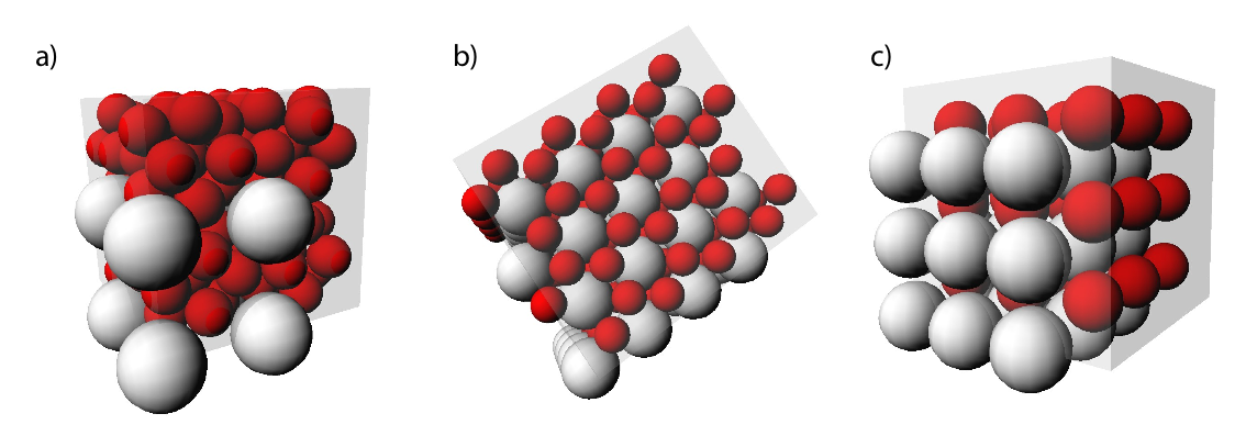
Figure 1: The three binary structures considered in this work, with the A particles shown as pale spheres, B particles shown as darker spheres, and the simulation cell shown as a translucent box. a) The AB13 structure consists of a simple cubic lattice of large spheres with icosahedral clusters of 13 B particles in the body-center of each cell. The 112 particle unit cell contains 8 B-clusters arranged in alternating orientations, where the clusters are rotate by $90^{\circ}$ between adjacent sub-cells. b) In AB2, hexagonal close-packed layers of A particles are stacked directly on top of each other, with a honeycomb pattern of B particles places in the interstitial sites between the A layers. c) The AB(CsCl) structure, consisting of two interlaced simple cubic lattices, with the B particles at the body-centre of the A cube.

These complex lattices have also seen in systems that bear little resemblance to hard-spheres, such as rare gas solids Layer2006 , nanocrystals Redl:2003aa , charge-stabilised colloids Royall2006 , and block copolymer micelles Abbas:2006aa . At first, it is surprising that these structures, particularly the highly complex AB13 superlattice, should form spontaneously in such a wide range of systems. However, it appears that entropic effects of hard-sphere packing are sufficient to stabilise these structures.

Previously, the lattice switch approach has been used for the free energy difference between two candidate structure for a single species. Two-species phase behaviour is more complicated, as the stable state of a binary system may consist of co-existing phases of different compositions, at equal pressures and chemical potentials. Therefore, instead of just comparing free energy of pairs of candidate phases, we must to evaluate the absolute free energies of all competing phases so that the overall phase diagram can be constructed. The basic approach has been presented in BARTLETT1990a by Bartlett, who considered only the fluid and pure (face-centered cubic A or B) crystal phases. We shall follow the work of Eldridge et al ELDRIDGE1993 ; ELDRIDGE1993b ; ELDRIDGE1995 ; Eldridge:1993aa and Cottin and Monson COTTIN1995 ; COTTIN1995a and also include AB2, AB13 and AB(CsCl) as candidate two-component crystals. In the Eldridge ELDRIDGE1993 work, the stability of AB2 and AB13 for binary hard spheres was determined using the thermodynamic integration method of Frenkel and Ladd FRENKEL1984 , with further details of the AB2 calculations in ELDRIDGE1993b and AB13 in Eldridge:1993aa . These results show general agreement with the experimental systems, but suggest that AB2 is kinetically repressed at the AB2 1:2 stoichiometry, as it only appears at higher concentrations of B particles Schofield2005 .

Theoretical studies of AB2, AB13 & AB(CsCl) have been also carried out via cell theory COTTIN1995 ; COTTIN1995a , and density functional theory (DFT) XU1992 ; DENTON1990 ; SMITHLINE1987 . For AB2 and AB13, the results are generally consistent with both the integration method and experimental results, although some minor differences remain. In particular, the range of stability of AB13 is computed via cell theory to be $0.61\geq\alpha\geq 0.54$ COTTIN1995a , whereas the integration method finds AB13 to be stable over the range $0.626\geq\alpha\geq 0.474$ Eldridge:1993aa . Although the latter work does not consider the possibility that AB2 is more stable than AB13 over this range of $\alpha,$ it is notable that the range of stability determined by integration methods is consistent with the range of observation of AB13 found in the experimental work presented in Schofield2005 .

The case of the AB(CsCl) structure is somewhat less clear. The close-packed density of this structure peaks at $\alpha=0.732$, and so may compete with the slightly denser FCC structure, and indeed metastable CsCl has been observed experimentally of at $\alpha=0.736$ in Schofield:2001bv . The stability of this structure has not been ascertained by integration methods: it was not considered to be a valid candidate structure in ELDRIDGE1995 . The cell theory work in COTTIN1995a did not find CsCl to be stable for any $\alpha$, but DFT results have shown metastablity DENTON1990 , and even stablity SMITHLINE1987 . However, the work in SMITHLINE1987 did not consider full phase separation into coexisting A and B FCC crystals; they only consider a fluid co-existing with a crystal phase made up of randomly distributed A and B particles, but rich in A, and the fluid composition appears to be fixed at 1:1. Interestingly, the AB(CsCl) structure has been stabilised experimentally by using oppositely charged colloids Leunissen2005 ; Bartlett2005 ; Hynninen2006a ; Royall2006 . Moreover, BCC is the lowest energy arrangement for charged monodisperse particles, so even if the AB(CsCl) structure is only metastable in general, it is possible that a small amount of charge transfer between particles or between particles and fluid is enough to stabilise the structure.

For even smaller sphere size ratios ($\alpha\lesssim 0.44$), the situation becomes more complicated as additional structures start to appear (e.g. AB(rocksalt) Trizac1997 ) and because, at lower volume fractions (or sufficiently low $\alpha$), the small spheres are free to move from site to site within the crystal of larger spheres. Such systems are not well suited to examination via the lattice-switch approach, as the algorithm would have to be modified heavily in order to cope in the free movement of small spheres. At smaller size ratios still, the success of the perturbative approach Velasco1999 suggests that it is best to model the presence of very small spheres via a depletion potential.

Given the range of results that exist for binary hard spheres, it provides an excellent testing ground for the extension of the lattice-switch approach to multi-component systems. As our primary concern is simply to extend the lattice-switch technique to the binary system, it makes sense to choose a particular value of $\alpha$ to examine, instead of trying to explore a whole range of diameter ratios before the correctness of the approach has been determined. We have chosen to examine the stability of AB2 and AB13 at $\alpha=0.58$, as there has been a large amount of theoretical and experimental work published for that particular diameter ratio. Furthermore, due to the ambiguity concerning the stability of the AB(CsCl) structure, we shall also use the lattice-switch approach to examine the stability of AB(CsCl) relative to the fluid phase and phase-seperated solid state at $\alpha=0.73$.

II Formulation

We consider a system of N particles, of spatial coordinates $\{\vec{r}\}$ and diameters $\{\sigma\},$ confined within a volume V, and subject to periodic boundary conditions. The configurational energy for this system of hard spheres has the form

$$E(\{\vec{r}\})=\left\{\begin{array}[]{l}0\textrm{ if }r_{ij}\leq\sigma_{ij}\;\forall\;i,j,\\ \infty\textrm{ otherwise, }\end{array}\right.$$ (1)

where $r_{ij}=\left|\vec{r_{i}}-\vec{r_{j}}\right|$ and $\sigma_{ij}=\frac{1}{2}\left(\sigma_{i}+\sigma_{j}\right)$. Each microstate has a Boltzmann weight $\exp[-\beta E]$, and so the total configurational weight associated with this system can be written as

$$\Omega(N,V)=\prod_{i}\left[\int_{V}d\vec{r_{i}}\right]\prod_{\langle ij\rangle}\Theta(r_{ij}-\sigma_{ij}),$$ (2)

where $\Theta(x)\equiv 1(0)$ for $x\geq 0(<0)$, and the product on $\langle ij\rangle$ extends over all particle pairs. The associated entropy density is

$$s(N,V)\equiv\frac{1}{N}\ln\Theta(N,V).$$ (3)

This formulation describes the total entropy, integrating over all possible positions and so over all possible phases. In order to compare the statistical weights of the configurations associated with individual (candidate) phases, we must formulate a constraint that identifies a configuration as ‘belonging to’ a given phase. To do this, we decompose the particle position coordinates into a sum of ‘lattice’ and ‘displacement’ vectors:

$$\vec{r_{i}}=\vec{R_{i}^{\mathcal{A}}}+\vec{u_{i}},$$ (4)

where $\{\vec{R}\}_{\mathcal{A}}\equiv\vec{R_{i}^{\mathcal{A}},i=1,...,N}$ forms a set of fixed vectors associated with the crystal structure labeled $\mathcal{A}$. This set is defined as the orthodox crystallographic lattice convolved with the orthodox basis, but will be referred to here as simply the ‘lattice vectors’. In previous work the coordinates $r_{i}$ have denoted a pure phase arrangement of the particles. However, it is possible for $\mathcal{A}$ to represent a two-phase mixture or for particle sizes to be changed in the switch. We are thus able to initialise a simulation within a particular phase, using the appropriate set of lattice vectors ($\{\vec{R}\}_{\mathcal{A}}$) and diameters ($\{\sigma\}_{\mathcal{A}}$) for that phase, just by setting $\vec{u_{i}}=\vec{0}\;\forall\;i$. We can now use a simple spatial criterion to decide whether a particular configuration belongs to the same phase as the simulation progresses. Periodically, throughout the simulation, the particles are checked to determine whether, after having taken any centre-of-mass drift into account, $\vec{u_{i}}$ is comparable to the interparticle spacing (for more details, see section III.3). This can only happen if the particles have been rearranged and the structure has been modified. so provides a robust criterion for ensuring that a set of microstates belong to the same macrostate. We note that this restriction of the configurational integral to pure perfect phases erases contributions from equilibrium concentrations of lattice defects, for example lattice vacancies, however for the systems in question such defects are extremely rare and make no significant contribution to total free energy Bowles:1994aa .

By performing this coordinate decomposition (eq. 4), we have effectively changed our stochastic variables from being $\{\vec{r}\}$ to $\left[\{\vec{u}\},\mathcal{A}\right]$, operating under a modified configuration energy function (c.f. eq. 1) of the form

$$E(\{\vec{u}\},\mathcal{A})=\left\{\begin{array}[]{l}0\textrm{ if }r_{ij}\leq\sigma_{ij}\;\forall\;i,j,\\ \infty\textrm{ otherwise, }\end{array}\right.$$ (5)

where the lattice label $\mathcal{A}$ dictates the choice of lattice vectors via $r_{ij}(\{\vec{u}\},\mathcal{A})=\left|\vec{(R_{i}^{\mathcal{A}}}+\vec{u_{i}})-\vec{(R_{j}^{\mathcal{A}}}+\vec{u_{j}})\right|$ and diameters via $\sigma_{ij}(\mathcal{A})=\frac{1}{2}\left(\sigma_{i}^{\mathcal{A}}+\sigma_{j}^{\mathcal{A}}\right)$. The configuration weight associated with a particular structure can now be written as

$$\Omega(N,V,\mathcal{A})=\prod_{i}\left[\int_{\mathcal{A}}d\vec{r_{i}}\right]\prod_{\langle ij\rangle}\Theta(r_{ij}-\sigma_{ij}),$$ (6)

where $\int_{\mathcal{A}}$ signifies integration subject to the single-phase constraint. The associated entropy density becomes

$$s(N,V,\mathcal{A})\equiv\frac{1}{N}\ln\Omega(N,V,\mathcal{A})$$ (7)

Once we construct a simulation capable of visiting the two different phases ($\mathcal{A},\mathcal{B}$), the entropy difference between them can be determined as:

$$\Delta s_{\mathcal{\mathcal{A}B}}\equiv s(N,V,\mathcal{A})-s(N,V,\mathcal{B})=\frac{1}{N}\ln\mathcal{R}_{\mathcal{A}\mathcal{B}}(N,V),$$ (8)

where

$$\mathcal{R}_{\mathcal{A}\mathcal{B}}(N,V)=\frac{\Omega(N,V,\mathcal{A})}{\Omega(N,V,\mathcal{B})}=\frac{P(\mathcal{A}|N,V)}{P(\mathcal{B}|N,V)}.$$ (9)

Here $P(\mathcal{A}|N,V)$ is the joint probability that a system free to visit both structures will be found in the $\mathcal{A}$ structure.

III Implementation and Methodology

III.1 Defining the structures and the switch

To evaluate the free energy of a particular binary crystal, we need to perform a lattice switch simulation capable of visiting the target phase, $\mathcal{A}$, and some reference phase, $\mathcal{B}$. As an accurate semi-empirical expression for the free energy of a monodisperse hard sphere FCC crystal has been determined by Alder et al ALDER1964 ; BJA1968:MDfccvhcpHS , we choose this structure to be our usual reference state. A lattice switch which kept the diameters of the particles fixed (such that $\{\sigma\}_{\mathcal{A}}\equiv\{\sigma\}_{\mathcal{B}}$), would require either a single simulation box containing co-existing crystals of A and B particles (and thus associated interfacial effects, making for a poor reference system) or two separate boxes corresponding to separate A and B crystals. This latter approach can be made to work, but the complexity associated with adding a second simulation cell is unnecessary when the two cells are being used to simulate two identical structures that differ only in scale (by $\alpha)$. A simpler option is to allow the diameters to change during the switch, turning all $\sigma_{B}$ particles in the mixed phase into particles of diameter $\sigma_{A}$, allocated different sites on a single shared FCC lattice. This creates a switch between a binary crystal and a single crystal, and ensures that the number of degrees of freedom in each system is the same. Furthermore, as the free-energy difference between FCC and HCP is accurately known ABD2000:LSMCmethod , we are free to use either close-packed structure as a reference crystal, which affords us a little more flexibility when it comes to choosing system sizes. The system sizes used are shown in Table 1.

	Target Crystal		Reference Crystal		Runtime	Runtime	Runtime
N	Structure	Dimensions	Structure	Dimensions	MCS [EOS]	MCS [WF]	MCS [DF]
112	AB13	$1\times 1\times 1$	HCP	$4\times 7\times 4$	$5\times 10^{5}$	$10^{6}\;[40]$	$4\times 10^{6}[8]$
896	AB13	$2\times 2\times 2$	FCC	$8\times 8\times 14$	$5\times 10^{5}$	$6\times 10^{6}\;[240]$	$6\times 10^{6}[10]$
192	AB2	$4\times 4\times 4$	FCC	$8\times 4\times 6$	$10^{6}$	$10^{6}\;[40]$	$4\times 10^{6}\;[80]$
648	AB2	$6\times 6\times 6$	FCC	$8\times 9\times 9$	$10^{6}$	$5\times 10^{6}\;[200]$	$2\times 10^{6}\;[200]$
54	CsCl	$3\times 3\times 3$	FCC	$6\times 3\times 3$	$5\times 10^{5}$	$10^{6}\;[40]$	$4\times 10^{6}\;[40]$
128	CsCl	$4\times 4\times 4$	HCP	$8\times 4\times 4$	$5\times 10^{5}$	$2\times 10^{6}\;[80]$	$5\times 10^{6}\;[20]$
432	CsCl	$6\times 6\times 6$	FCC	$8\times 6\times 9$	$5\times 10^{5}$	$3\times 10^{6}\;[120]$	$8\times 10^{6}\;[40]$

Table 1: Structures and sizes used in this work. For FCC, HCP and AB2, the unit-cells were oriented so that the close-packed layers were lying in the x-y plane. The cubic cells of AB13 and CsCl were made commensurate with the simulation cell. The run times are shown for determining the equation of state (EOS), the weight function (WF) and the free-energy difference (DF), in units of Monte Carlo sweeps (MCS). Numbers in square brackets indicates the largest number of blocks the run was split into for block analysis. For all structures and sizes, 20,000 MCS runs were used to equilibrate the constant pressure runs, while the constant volume simulations needed just 5,000 MCS for equilibration.

Once the crystal lattices have been chosen, one must choose a site mapping between crystals $\mathcal{A}$ and $\mathcal{B}$ . In the previous lattice-switch work for FCC and HCP structures more efficient switches which preserved close-packed planes were used. However, for binary-to-single-lattice switches, there are no such obvious similarities, therefore, we mapped sites between crystals at random.

To predict the equilibrium phase behaviour, we must first determine the Gibbs free energy of all the candidate phases, as a function of the pressure, $P^{\star}=P\sigma_{A}^{3}/kT$, and the composition, $X=N_{B}/(N_{A}+N_{B})$, where $N_{A}$ and $N_{B}$ are the numbers of A and B particles respectively. Naturally, we would seek to measure the Gibbs free energy directly via a lattice-switch simulation carried out in the constant pressure ensemble. However, when attempting to switch between the pure and the binary crystals using a single simulation cell, the fact that the equilibrium cell size is very different for these two structures means that the switch becomes ineffective. The lattice-switch only updates the lattice and the diameters, not the cell parameters, and therefore performing the switch from the reference lattice involves attempting to transform an equilibrium density pure crystal into a loosely packed binary crystal (as reducing the diameter of so many particles vastly increases the available volume). The conjugate move requires a transformation from an equilibrium density binary crystal to a pure crystal at such a high density that it is likely that all particles overlap. To facilitate either switching move, the volume of the simulation cell would have to be dilated so far that the system would rapidly melt, and indeed such a switch cannot be made to work in practice. It is possible, at least in principle, to overcome this limitation by adding an explicit volume dilation to the switch, so that the cell dimensions, the lattice and the diameters are all changed simultaneously. However, adding a volume transformation factor affects the probability of sampling the two phases in a non-trivial way. For example, a dilation to a large cell will almost always be accepted, whereas the compression to a small cell will be difficult to achieve. This will bias the measured free energy difference by a factor which could be determined by careful application of the mapping transformation matrix approach outlined in ABD2000:LSMCmethod , but this introduces a number of computational overheads, and the slow switching rate mitigates against gathering good statistics.

All these issues can be avoided in the constant volume ensemble by keeping the density fixed when switching between the reference and target structures, thus ensuring that the displacements are reasonable in both phases because the distances between particles are comparable in both phases under these conditions.

III.2 Simulation Methodology

To estimate the Gibbs free energy, three simulations were carried out for each state point. The first was a single phase constant pressure (NPT) simulation, used to estimate the equilibrium density and cell parameters (c/a ratio) for each binary crystal, at each pressure. Then, two lattice-switch NVT simulations were performed at the volume fractions and c/a ratios determined from the NPT simulations. The lattice switch attempts to transform between the target crystal (at the target density and c/a ratio) and a pure FCC crystal (at the same density, but with c/a = 1.0). The first run is used to evaluate the multicanonical weight function and the second uses this function to determine the free energy difference between the crystals (see section III.3 for more details).

Having determined the cell proportions, the density, and the Helmholtz free energy difference between the two structures ($\Delta F$) for a range of pressures, we can then build the absolute free energy of the binary crystal by adding in the free energy of the pure phase. To determine this, we integrate the Alder equation of state ALDER1964 ; BJA1968:MDfccvhcpHS ; YOUNG1979 ,

$$\frac{PV}{NkT}=\frac{3}{V^{\star}-1}+2.566+0.55(V^{\star}-1)-1.19(V^{\star}-1)^{2}+5.95(V^{\star}-1)^{3},$$ (10)

with respect to the reduced volume $V^{\star}=V/V_{0}$ (where $V_{0}$ is the close packed volume, $N\sigma^{3}/\sqrt{2}$). This yields the Helmholtz free-energy:

$$\frac{F_{ex}^{Alder}}{NkT}=-3\ln\left(\frac{V^{\star}-1}{V^{\star}}\right)+5.124\ln V^{\star}-20.78V^{\star}+\frac{19.04}{2}V^{\star 2}-\frac{5.95}{3}V^{\star 3}+C_{4}+1,$$ (11)

where, following YOUNG1979 , the constant of integration $C_{4}$ is set to $15.05$. The Gibbs free energy can be constructed from the Helmholtz form via:

$$G_{ex}=F_{ex}^{Alder}+\Delta F+PV-1-\ln\left[\frac{PV}{NkT}\right]$$ (12)

where the last two terms arise from the difference between the Gibbs and Helmholtz free energies for an ideal gas. To compute the phase diagrams based on these free energies, we follow the approach of Bartlett BARTLETT1990 and assume that the particles are immiscible in the solid phases, and that the binary fluid behaviour can be described accurately by the Mansoori equation MANSOORI1971 . At each pressure, the densities of the candidate phases are determined from the equations of state. From these densities, the Gibbs free energies and chemical potentials of the competing phases can be determined for each constant pressure line. The condition of equal chemical potentials is then applied along the constant pressure line, where the the coexistence between the crystal phases and the Mansoori fluid is estimated from the chemical potentials of each species in the fluid via (see COTTIN1995a ):

$$\mu_{A}^{f}+n\mu_{B}^{f}=(1+n)\times G(AB_{n}),$$ (13)

where $\mu_{A}^{f}$ and $\mu_{B}^{f}$are the chemical potentials determined from the Mansoori fluid for the A and B particles respectively, and $G(AB_{n})$ is the Gibbs free energy of the solid phase that has $n$ B particles for each A particle.

III.3 Multicanonical Biassed Monte Carlo procedure

In general, a lattice switch move from a zero-overlap microstate in one phase is unlikely to map onto a zero-overlap microstate in the other. Therefore, the simulation must monitor not only which phase the is currently being explored, but also how close the simulation is to being able to perform the lattice switch. To find a suitable order parameter, we first let $M(\{\vec{u}\},\mathcal{A})$ denote the number of overlapping pairs of particles associated with the displacements $\{\vec{u}\}$, within the structure $\mathcal{A}$. We can then define the overlap order parameter:

$$\mathcal{M}(\{\vec{u}\})\equiv M(\{\vec{u}\},\mathcal{B})-M(\{\vec{u}\},\mathcal{A}),$$ (14)

where $\mathcal{M}$ is necessarily $\geq 0$ ($\leq 0$) for realizable configurations of the $\mathcal{A}$ ($\mathcal{B}$) structure. To ensure that the simulation can reach the so-called gateway states ($\mathcal{M}=0$), we apply the multi-canonical Monte Carlo method BAB1999:mcmcrev as a way of biasing the simulation in a controlled fashion. To this end, we augment the system energy function such that

$$\mathcal{E}(\{\vec{u}\},\mathcal{A})=E(\{\vec{u}\},\mathcal{A})+\eta(\mathcal{M}(\{\vec{u}\})),$$ (15)

where $\eta(\mathcal{M}),\mathcal{M}=0,\pm 1,\pm 2,...$ constitute a set of multicanonical weights BAB1999:mcmcrev . Given that a suitable weight function can be determined (see below), the canonical distribution $P(\mathcal{M}|N,V)$ can be estimated from the measured multicanonical distribution $P(\mathcal{M}|N,V,\{\eta\})$ with the identification

$$\mathcal{R}_{\mathcal{AB}}(N,V)=\frac{\sum_{\mathcal{M}>0}P(\mathcal{M}|N,V)}{\sum_{\mathcal{M}<0}P(\mathcal{M}|N,V)}=\frac{\sum_{\mathcal{M}>0}P(\mathcal{M}|N,V,\{\eta\})e^{\eta(\mathcal{M})}}{\sum_{\mathcal{M}<0}P(\mathcal{M}|N,V,\{\eta\})e^{\eta(\mathcal{M})}}.$$ (16)

Here, the exponential reweighting maps the multicanonical distribution onto the canonical, unfolding the bias associated with the weights.

The multicanonical weights are determined from non-equilibrium calculations, which are fast and give a fair approximation to the equilibrium situation. We conduct a series of separate Monte Carlo simulations, where the particle displacements (and therefore $\mathcal{M}$) are reset to zero at the start of each. As these simulations will each relax to the equilibrium $\mathcal{M}$ values, this forces the overall run to explore the full range of $\mathcal{M}$. Throughout this sequence of simulation, the program monitors and accumulates the macrostate transition probability matrix, as described in Smith:1996aa , and at the end of the whole run, an estimate of the weight function is determined from the transitions probabilities by a simple shooting method Jackson2001 . This weight function is then used for the second NVT run, during which the time spent in each phase is recorded (with the biasing taken into account), and automatically block-analysed to produce an estimate of the free-energy difference. The actual timings varied depending on the target system and the number of particles, and are shown in Table 1.

The simulations operated under the usual Metropolis algorithm 1953NM:MC , using random numbers generated by the Mersenne Twister algorithm 272995 , as implemented in RngPack, version 1.1a Houle2003 . For each move, a sphere is chosen at random, and a trial displacement is generated by taking the displacement of that particle $\vec{u_{i}}$ and adding a random three-dimensional vector $\Delta\vec{u_{i}}$ drawn uniformly from a cube of fixed size. The update in the displacement is accepted according to the usual Metropolis prescription:

$$p_{a}(\{\vec{u}\}\rightarrow\{\vec{u}\}+\Delta\vec{u_{i}})=\min\{1,\exp[-(\mathcal{E}(\{\vec{u}+\Delta\vec{u_{i}}\},\mathcal{A})-\mathcal{E}(\{\vec{u}\},\mathcal{A}))]\}.$$ (17)

Therefore, moves that would lead to overlaps in the current phase are always rejected, and moves that would alter the number of overlaps in the conjugate phase are accepted or rejected based on the multicanonical weights. The magnitude of $\Delta\vec{u_{i}}$ was automatically adjusted to yield an acceptance rate of about one third, as this has been shown previously to produce an acceptable rate of decorrelation in $\mathcal{M}$ Jackson2001 . When $\mathcal{M}=0$, the lattice-switch move is attempted once per Monte Carlo Sweep (MCS) (i.e. once every N particle moves) on average, and is always accepted as there is no energy cost or multicanonical weight difference associated with this move.

Due to the short-range nature of the hard sphere interaction, the calculation of $E(\{\vec{u}\},\mathcal{A})$ does not need to extend over all $N^{2}$ particle pairs. To make the simulation more efficient, each particle only checks for interactions with its neighbours, up to a maximum interaction distance of 1.5 unit cells (i.e. 1.5 times the A-A separation). There are two lists of neighbours for each particle: one for each phase. As mentioned in section II, we require a criterion to determine whether structure is stable, and the simulation achieves this by periodically scanning the system for particles that have moved further than the near neighbour distance away from their site (after having taken any centre of mass diffusion into account). If this is observed to happen at any point during any simulation at a given pressure, then the structure is considered unstable, and no longer considered as a candidate structure at that pressure.

To establish the equations of state for these systems, a number of constant pressure simulations were also performed. In this case, the simulation cell parameters (the lengths of the sides of the cell, and therefore the volume) can fluctuate during the simulation. Such moves are accepted with probability:

$$p_{a}(V\rightarrow V^{\prime})=\min\{1,\exp[-(\mathcal{E}(\{\vec{u}\}^{\prime},\mathcal{A})-\mathcal{E}(\{\vec{u}\},\mathcal{A}))-P^{\star}\Delta V+N\ln(V^{\prime}/V)]\},$$ (18)

where $V^{\prime}$ is the volume associated with the trial move. Of course, this cell-size dilation can change $\mathcal{E}$ globally, and so an expensive energy calculation must be carried out for each trial volume move. Volume moves were attempted at random, once per MCS on average. The maximum size of the random volume-dilation is automatically adjusted so that the acceptance rate for volume moves is about one half, which produces an acceptable rate of exploration of the volume parameter space Jackson2001 .

IV Results

IV.1 Pressure curves and stability

The equations of state, as measured by Monte Carlo simulation in the constant pressure ensemble, are shown in Figure 2. The agreement with the data presented in Eldridge:1993aa indicates that the Molecular Dynamics simulation presented there used the smaller ($N=112$) system size when computing the equation of state. Also, the close agreement between the Alder equation of state ALDER1964 and the simulated FCC crystal is clear. However, we note that while the Alder form (eq. 10) provides a reliable estimate of the equation of state, the individual terms are difficult to reproduce. Despite having determined the density of the FCC structure at each pressure to within at least $0.1\%$, attempting to fit an equation of the Alder form to this data led to a poorly-determined fit that only reproduced the original terms to within one significant figure. It is therefore clear that a much larger range of pressures must be used to determine Alder-style equations of state for these structures, and given that quite a modest range of pressures was explored in the original work BJA1968:MDfccvhcpHS , it is not clear that the parameterization supplied in eq. 10 is a particularly accurate one.

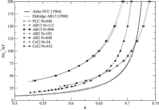
Figure 2: Equations of state determined in the constant pressure ensemble, measuring the density as a function of the pressure. Errors in the density estimates are smaller than the symbol size. The Alder equation of state for the pure crystal ALDER1964 is shown as a solid line, and the equation of state for AB13 as observed in Eldridge:1993aa is shown as a solid gray line.

During the equation of state simulations, the cell proportions were also monitored and Figure 3 shows the results in terms of the c/a ratio. As expected on symmetry grounds, the AB13 and CsCl crystals are stable at $c/a=1$. However, the AB2 crystal tends to expand in the direction perpendicular to the alternating stacking planes of A and B particles, and the degree of expansion found here is consistent with the results presented in ELDRIDGE1993b . The c/a ratio decreases as the pressure is lowered towards the fluid region, and as the simulations approach the melting point, the fluctuations in the volume and aspect ratio of all the crystals become large as the structures start to break down. As noted earlier, this break-down condition discounts extended metastability and the possibility that the structure may be stabilised by some equilbrium concentration of defects, and so provides an upper bound on the actual limit of stability of the structure.

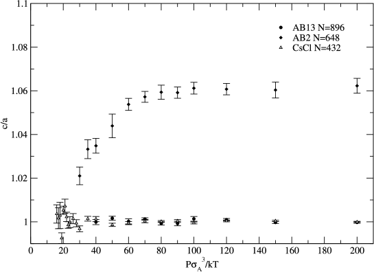
Figure 3: Observed $c/a$ ratios for the target phases.

IV.2 Free energies

The free energy difference between the reference (FCC or HCP) and target crystals AB2 and AB13 at $\alpha=0.58$, and for AB(CsCl) at $\alpha=0.73$ are shown in Figure 4. In all cases, the free energy difference between FCC and HCP $(\approx 1\times 10^{-3}kT$ per particle) is so small that it cannot be resolved on the scale of these plots. The AB2 and AB13 structures are lower in free energy than the FCC crystals for all densities at these size ratios.

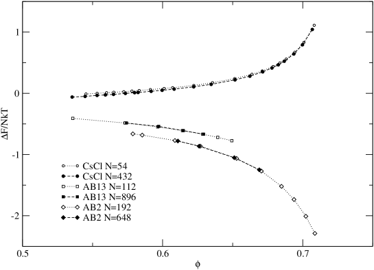
Figure 4: The raw Helmholtz free energy difference per particle between the reference FCC and target AB2 and AB13 crystals at $\alpha=0.58$, and AB(CsCl) at $\alpha=0.73$, as measured by the lattice switch simulations. The final data points at low $\phi$ indicate the lowest density at which the structure was determined to be stable. The points at the high density end indicate the upper limit of the chosen pressure range explored by the simulations. Some simulations were performed at larger system sizes, as shown here, and indicated that the overall form of the free energy difference does not depend strongly on the system size.

Figure 4 also shows that the AB(CsCl) structure has a significantly higher Helmholtz free energy than FCC at high densities, the difference falls rapidly as the density is lowered towards melting. However, it is important to remember that the AB(CsCl) structure is not competing with a pure FCC crystal, but with one or more coexisting phases at equal pressures and chemical potentials. Figure 5 illustrates this by comparing the Gibbs free energy of AB(CsCl) with those of the competing phases - a Mansoori fluid, a pure FCC crystal coexisting with a B-rich Mansoori fluid, and a dual crystal state made up of separate A and B FCC crystals. The AB(CsCl) structure is clearly not stable over this range, and this result compares favourably with results from DFT calculations in DENTON1990 and via cell theory in COTTIN1995a . However, we note that the free energy difference is quite small, and so a small amount of charge asymmetry may be sufficient to stabilise the structure in the low density solid phase.

Figure 5: Gibbs free energies as a function of pressure for AB(CsCl) $\alpha=0.72$ at a fixed composition of $X=0.5$. The Gibbs free energies of the Mansoori fluid, the pure A FCC crystal coexisting with a Mansoori fluid, and the dual FCC A and B crystal phases are also shown. Finite size effects cannot be resolved on this plot.

For all structures, the free energy difference measured in the constant density ensemble shows very little dependence on system size, and even rather small systems provide reasonable estimates of the free energy difference with respect to FCC. To allow comparison with the literature results, the Helmholtz free energies of the structures for $\alpha=0.58$ are shown in figure 6, and the Gibbs free energies (computed via eq. 12) are shown in Figure 7. The lattice switch results are in clear agreement with the results determined via integration methods Eldridge:1993aa ; ELDRIDGE1993b , and with the DFT results presented in XU1992 and the cell theory results in COTTIN1995a . For clarity, Figure 6 only includes the results presented in Eldridge:1993aa ; ELDRIDGE1993b and omits the almost identical results of COTTIN1995 ; COTTIN1995a .

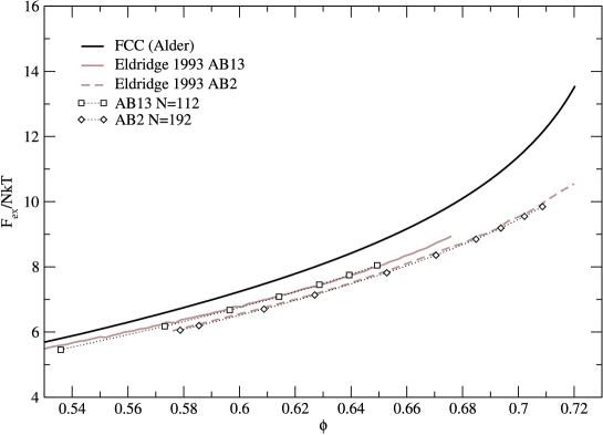
Figure 6: The excess (i.e. with respect to an ideal gas) Helmholtz free energies of AB2, AB13 and FCC at $\alpha=0.58.$ Data from literature for AB2 ELDRIDGE1993b and AB13 Eldridge:1993aa is also shown for comparison.

Figure 7: Gibbs free energies for AB2 and AB13 at $\alpha=0.58$. The Gibbs free energies of Mansoori fluid and the A FCC crystal coexisting with a B-rich Mansoori fluid at the appropriate compositions are also shown. Finite size effects cannot be resolved on this plot.

IV.3 Phase diagrams

Following the prescription outlined in section III.2, the lattice switch data were used to predict the pressure-composition phase diagram for the binary hard sphere system at $\alpha=0.58$, and the results are shown in Figure 8. The corresponding partial volume-fraction phase diagram is shown in Figure 9. Both these figures agree well with the established results ELDRIDGE1993 ; COTTIN1995a , although the partial volume fraction phase diagram does not extend to as high densities as the one published in ELDRIDGE1993 due to the limited range of pressures explored in the current work.

Figure 8: P-X Phase Diagram at $\alpha=0.58$, determined from the lattice switch results using the methodology described in section III.2.

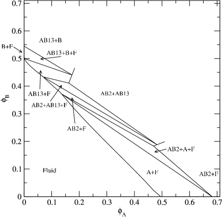
Figure 9: Partial volume fraction phase diagram, built from the P-X results shown in Figure 8 using the equation of state data to determine the densities of coexisting phases along each P-X coexistence line.

V Discussion

We have presented a method by which the lattice switch approach can be applied to binary mixtures, and applied it to binary hard sphere system. The technical innovation introduced here involves including a rescaling of particle sizes in the switch. Combining our free energy differences enables us to build a phase diagram which is in excellent agreement with previous theoretical results at the size ratio 0.58. The only errors in the lattice-switch MC approach come from finite size effects and sampling errors, which are easy to quantify. The phase diagrams themselves rely on the Alder and Mansoori equations of state for the FCC and liquid free energies respectively.

We also investigated the experimentally reported CsCl phase at size ratio 0.73, and found it to be unstable compared to phase-segregated FCC or the liquid. However the energy differences are small, and it is possible that either charge effects or polydispersity may be responsible for the experimental observation of this structure.

The dependence upon the Alder crystal is perhaps unfortunate, as it is unclear how accurate the parameters of this equation of state are. However, the Alder equation of state is dominated by the leading term and rather insensitive the poorly-determined parameters. Our results are in good agreement with the literature, including those ELDRIDGE1993 which do not depend on the Alder formulation (due to using an Einstein crystal as a reference state). In the same vein, building a lattice-switch mapping to an analytically soluble reference crystal would also allow the use of the Alder equation of state to be avoided. This Hamiltonian-switch approach could map from an Einstein crystal or single-occupancy cell model to the target potential and structure, and would allow absolute free energies to be measured directly.

Other future work includes lower size ratio, although as mentioned before, the mobile smaller spheres will present challenges, although it may be possible to use tethers, in a manner similar to that employed for the fluid-solid transition Wilding2002 . Also, these structures have been observed for noble gas mixtures Layer2006 , and this could be investigated by generalising this approach in the same manner as the extension to soft-potentials of the original lattice switch approach Jackson:2002aa .

- [1] J Keplar. Strena sue de nuive sexangula. 1611.
- [2] TC Hales and SP Ferguson. The kepler conjecture, 1998. Details of Keplar’s conjecture and it’s solution can be found at http://www.math.lsa.umich.edu/ hales/countdown/.
- [3] AD Bruce, NB Wilding, and GJ Ackland. Free energy of crystalline solids: A lattice-switch monte carlo method. Physical Review Letters, 79(16):3002–3005, 1997. cond-mat/9706154.
- [4] D Frenkel and AJC Ladd. New monte-carlo method to compute the free-energy of arbitrary solids - application to the fcc and hcp phases of hard-spheres. Journal Of Chemical Physics, 81(7):3188–3193, 1984.
- [5] MD Eldridge, PA Madden, and D Frenkel. Entropy-driven formation of a superlattice in a hard-sphere binary mixture. Nature, 365(6441):35–37, 1993.
- [6] M. Eldridge, P. Madden, and D Frenkel. A computer-simulation investigation into the stability of the AB2 superlattice in a binary hard-sphere system. Molecular Physics, 80(4):987–995, 1993.
- [7] M. Eldridge, P. Madden, and D Frenkel. The stability of the AB13 crystal in a binary hard sphere system. Molecular Physics, 79(1):105–120, 1993.
- [8] AD Bruce, AN Jackson, GJ Ackland, and NB Wilding. Lattice-switch monte carlo method. Physical Review E, 61(1):906–919, Jan 2000. cond-mat/9910330.
- [9] NB Wilding and AD Bruce. Freezing by monte carlo phase-switch. Physical Review Letters, 85(24):5138–5141, 2000. cond-mat/0009062.
- [10] N Wilding. A new simulation approach to the freezing transition. Computer Physics Communications, 146(1):99–106, 2002.
- [11] A N Jackson, A D Bruce, and G J Ackland. Lattice-switch monte carlo method: application to soft potentials. Physical review E, Statistical, nonlinear, and soft matter physics, 65(3 Pt 2B):036710, Mar 2002.
- [12] Jeffrey Errington. Solid–liquid phase coexistence of the lennard-jones system through phase-switch monte carlo simulation. The Journal of Chemical Physics, 120(7):3130–3141, 2004.
- [13] G McNeil-Watson and N Wilding. Freezing line of the lennard-jones fluid: A phase switch monte carlo study. Journal Of Chemical Physics, 124(6):064504, 2006.
- [14] JL Barrat, M Baus, and JP Hansen. Density-functional theory of freezing of hard-sphere mixtures into substitutional solid solutions. Phys Rev Lett, 56(10):1063–1065, Mar 1986.
- [15] J Barrat, M Baus, and J Hansen. Freezing of binary hard-sphere mixtures into disordered crystals: a density functional approach. Journal of Physics C: Solid State Physics, 20(10):1413–1430, 1987.
- [16] J.V Sanders. Close-packed structures of spheres of two different sizes. i. observations on natural opal. Philosophical Magazine A (Physics of Condensed Matter, Defects and Mechanical Properties), 42(6):705–720, Dec 1980.
- [17] M.J Murray and J.V Sanders. Close-packed structures of spheres of two different sizes. ii. the packing densities of likely arrangements. Philosophical Magazine A (Physics of Condensed Matter, Defects and Mechanical Properties), 42(6):721–740, Dec 1980.
- [18] P Bartlett, RH Ottewill, and PN Pusey. Freezing of binary-mixtures of colloidal hard-spheres. Journal Of Chemical Physics, 93(2):1299–1312, 1990.
- [19] P Pusey. Phase-behavior and structure of colloidal suspensions. Journal Of Physics-Condensed Matter, 6:A29–A36, 1994.
- [20] MD Eldridge, PA Madden, PN Pusey, and P Bartlett. Binary hard-sphere mixtures: a comparison between computer-simulation and experiment. Molecular Physics, 84(2):395–420, 1995.
- [21] N Hunt, R Jardine, and P Bartlett. Superlattice formation in mixtures of hard-sphere colloids. Physical Review E, 62(1):900–913, 2000.
- [22] A Schofield, P Pusey, and P Radcliffe. Stability of the binary colloidal crystals ab(2) and ab(13). Physical Review E, 72(3):031407, 2005.
- [23] M Layer, A Netsch, M Heitz, J Meier, and S Hunklinger. Mixing behavior and structural formation of quench-condensed binary mixtures of solid noble gases. Physical Review B, 73(18):184116, 2006.
- [24] F X Redl, K-S Cho, C B Murray, and S O’Brien. Three-dimensional binary superlattices of magnetic nanocrystals and semiconductor quantum dots. Nature, 423(6943):968–71, Jun 2003.
- [25] C Royall, M Leunissen, A Hynninen, M Dijkstra, and A van Blaaderen. Re-entrant melting and freezing in a model system of charged colloids. Journal Of Chemical Physics, 124(24):244706, 2006.
- [26] Sayeed Abbas and Timothy P Lodge. Superlattice formation in a binary mixture of block copolymer micelles. Phys Rev Lett, 97(9):097803, Sep 2006.
- [27] P Bartlett. A model for the freezing of binary colloidal hard-spheres. Journal Of Physics-Condensed Matter, 2(22):4979–4989, 1990.
- [28] X Cottin and PA Monson. A theory of solid-solutions and solid-fluid equilibria for mixtures. International Journal Of Thermophysics, 16(3):733–741, 1995.
- [29] X Cottin and PA Monson. Substitutionally ordered solid-solutions of hard-spheres. Journal Of Chemical Physics, 102(8):3354–3360, 1995.
- [30] H Xu. A density functional-study of superlattice formation in binary hard-sphere mixtures. Journal Of Physics-Condensed Matter, 4(50):L663–L668, 1992.
- [31] A Denton. Weighted-density-functional theory of nonuniform fluid mixtures - application to freezing of binary hard-sphere mixtures. Physical Review A, 42(12):7312–7329, 1990.
- [32] S Smithline. Density functional theory for the freezing of 1-1 hard-sphere mixtures. Journal Of Chemical Physics, 86(11):6486–6494, 1987.
- [33] A Schofield. Binary hard-sphere crystals with the cesium chloride structure. Physical Review E, 64(5), 2001.
- [34] M Leunissen, C Christova, A Hynninen, C Royall, A Campbell, A Imhof, M Dijkstra, R van Roij, and A van Blaaderen. Ionic colloidal crystals of oppositely charged particles. Nature, 437(7056):235–240, 2005.
- [35] P Bartlett and A Campbell. Three-dimensional binary superlattices of oppositely charged colloids. Physical Review Letters, 95(12):128302, 2005.
- [36] A Hynninen, M Leunissen, A van Blaaderen, and M Dijkstra. Cuau structure in the restricted primitive model and oppositely charged colloids. Physical Review Letters, 96(1):018303, 2006.
- [37] E Trizac, M Eldridge, and P Madden. Stability of the ab crystal for asymmetric binary hard sphere mixtures. Molecular Physics, 90(4):675–678, 1997.
- [38] E Velasco, G Navascues, and L Mederos. Phase behavior of binary hard-sphere mixtures from perturbation theory. Physical Review E, 60(3):3158–3164, 1999.
- [39] Richard Bowles and Robin Speedy. Cavities in the hard sphere crystal and fluid. Molecular Physics, 83(1):113–125, 1994.
- [40] B Alder. Studies in molecular dynamics. iii. mixture of hard spheres. Journal Of Chemical Physics, 40(9):2724, 1964.
- [41] BJ Alder, WG Hoover, and DA Young. Studies in molecular dynamics. v. high-density equation of state and entropy for hard-discs and spheres. Journal of Chemical Physics, 49(8):3688–3696, Oct 1968.
- [42] D Young. Studies in molecular-dynamics .17. phase-diagrams for step potentials in 2 and 3 dimensions. Journal Of Chemical Physics, 70(1):473–481, 1979.
- [43] G Mansoori. Equilibrium thermodynamic properties of misture of hard spheres. Journal Of Chemical Physics, 54(4):1523, 1971.
- [44] BA Berg. Introduction to multicanonical monte carlo simulations. Fields Institute Communications, 1999. cond-mat/9909236.
- [45] GR Smith and AD Bruce. Multicanonical monte carlo study of solid-solid phase coexistence in a model colloid. Phys Rev E Stat Phys Plasmas Fluids Relat Interdiscip Topics, 53(6):6530–6543, Jun 1996.
- [46] A.N Jackson. Structural Phase Behaviour Via Monte Carlo Techniques. PhD thesis, 2001.
- [47] N Metropolis, A Rosenbluth, M Rosenbluth, AH Teller, and E Teller. Equations of state calculations by fast computing machines. Journal of Chemical Physics, 21:1087, 1953.
- [48] Makoto Matsumoto and Takuji Nishimura. Mersenne twister: a 623-dimensionally equidistributed uniform pseudo-random number generator. ACM Trans. Model. Comput. Simul., 8(1):3–30, 1998.
- [49] Paul Houle. Rngpack 1.1a, http://www.honeylocust.com/rngpack/.