Stochastic resonance and heat fluctuations in a driven double-well system

Abstract

Abstract:  We study a periodically driven (symmetric as well as asymmetric)double-well potential system at finite temperature.  We show that mean heat loss by the system to the environment  (bath) per period of the applied field is a good quantifier of stochastic resonance.   It is found that the heat fluctuations over a single period are always larger than the work fluctuations.   The observed distributions of work and heat exhibit pronounced asymmetry near resonance.   The heat losses over a large number of periods satisfies the conventional steady-state fluctuation theorem,  though different relation exists for this quantity.

Key Words:  Stochastic Resonance,  Fluctuation Theorem
PACS numbers: 05.40.-a; 05.40.Jc; 05.60.Cd; 05.40.Ca

Corresponding Author: A.M. Jayannavar
Email address : jayan@iopb.res.in

I Introduction

Stochastic Resonance (SR) was discovered barely about two and half decades ago, yet it has proved to be very useful in explaining many phenomena in natural sciences[1-3]. SR refers to an enhanced response of a nonlinear system to a subthreshold periodic input signal in the presence of noise of optimum strength. Here, noise plays a constructive role of pumping power in a particular mode, that is in consonance with the applied field, at the cost of the entire spectrum of modes present in it. SR, so defined, leaves a lot of liberty as to what is the physical quantity that is to be observed which should show a maximum as a function of noise strength[4-23]. In other words, no unique quantifier of SR is specified. Also, in order that SR be a bonafide resonance the quantifier must show maximum as a function of frequency of the applied field as well. For instance, in a double-well system, hysteresis loop area, input energy or work done on the system in a period of the driving field and area under the first peak in the residence time (in a well) distribution are used to characterize SR as a bonafide resonance[4-17,19-22].

In the present work, motivated by recently discovered fluctuation theorems, we show that in an overdamped bistable system input energy per period as well as the energy absorbed per period by the system from the bath, i.e, the heat, can be used as quantifiers to study SR. Also, it is found that the relative variance of both the quantities exhibit minimum at resonance; that is, whenever input energy and heat show maximum as a function of noise strength (as also frequency), their respective relative fluctuations show minimum. This shows that at SR the system response exhibits greater degree of coherence. These fluctuations, however, are very large and often the physical quantities in question become non-self-averaging. We study some of these aspects in the light of the fluctuation theorems in the following sections. The fluctuation theorems are of fundamental importance to nonequilibrium statistical mechanics[24-46]. The fluctuation theorems describe rigorous relations for properties of distribution functions of physical variables such as work, heat, entropy production, etc., for systems far from equilibrium regimes where Einstein and Onsagar relations no longer hold. These theorems are expected to play an important role in determining thermodynamic constraints that can be imposed on the efficient operation of machines at nano scales. Some of these theorems have been verified experimentally[47-53].

II The Model

We consider the motion of a particle in a double-well potential $V(x)=-\frac{ax^{2}}{2}+\frac{bx^{4}}{4}$ under the action of a weak external field $h(t)=A\sin(\omega t)$. The motion is described by the overdamped Langevin equation[44]

$$\gamma\frac{dx}{dt}=-\frac{\partial U(x)}{\partial x}+\xi(t),$$ (1)

where $U(x)=V(x)-h(t)x$. The random forces satisfy $\langle\xi(t)\rangle=0$ and $\langle\xi(t)\xi(t^{{}^{\prime}})\rangle=2\gamma k_{B}T\delta(t-t^{{}^{\prime}})$, where $\gamma$ is the coefficient of friction, $T$ is the absolute temperature and $k_{B}$ is the Boltzmann constant. In the following we use a dimensionless form of equation(1), namely,

$$\frac{dx}{dt}=-\frac{\partial U(x)}{\partial x}+\xi(t),$$ (2)

where $U(x)=-\frac{x^{2}}{2}+\frac{x^{4}}{4}-xh(t)$, and the external field $h(t)=A\sin(\omega t)$. Now, $\xi(t)$ satisfies $\langle\xi(t)\xi(t^{{}^{\prime}})\rangle=D\delta(t-t^{{}^{\prime}})$, where $D=2k_{B}T$. All the parameters are given in dimensionless units  (in terms of $\gamma$, $a$ and $b$). We consider $A\ll 0.25$, so that the forcing amplitude is much smaller than the barrier height between the two wells.

Following the stochastic energetic formalism developed by Sekimoto[55], the work done by the external drive $h(t)$ on the system or the input energy per period (of time $\tau_{\omega}$) is defined as[21]

$$W_{p}=\int_{0}^{t_{0}+\tau_{\omega}}\frac{\partial U}{\partial t}dt$$

$$=-\int_{0}^{t_{0}+\tau_{\omega}}x(t)\frac{dh(t)}{dt}dt,$$ (3)

where $h(t)$ is the drive field which completes its period in time $\tau_{\omega}$. The completion of one period of $h(t)$, however, does not guarantee the system coming back to the same state as the starting one. In other words, $x(t+\tau_{\omega})$ need not be equal to $x(t)$ or $U(x,t+\tau_{\omega})$ may differ from $U(x,t)$. The work done over a period $W_{p}$ equals change in the internal energy $\Delta U=U(x,t_{0}+\tau_{\omega})-U(x,t_{0})$ and heat $Q$ absorbed over a period (first law of thermodynamics), i.e, $W_{p}=\Delta U_{p}+Q_{p}$. Since $x(t)$ is stochastic, $W_{p}$, $\Delta U_{p}$ and $Q_{p}$ are not the same for different cycles(or periods) of $h(t)$. The averages are evaluated from a single long trajectory $x(t)$ (eqn(3)). From the same calculations one can also obtain the probability distribution $P(W)$ and various moments of $W$. Similarly, appealing to the first law of thermodynamics as stated above we can obtain $P(Q_{p})$ and $P(\Delta U_{p})$ and their moments, where the subscript p indicates evaluation of the physical quantities over one period of the field. Numerical simulation of our model was carried out by using Huen’s method[56]. To calculate $W_{p}$ and $Q_{p}$ we first evolve the system and neglect initial transients. To get better statistics we calculate $W_{p}$, $Q_{p}$ for $10^{6}$ cycles. In some cases we evaluate $W$, $\Delta U$ and $Q$ over many periods, $n$, and calculate their averages, again, for $10^{6}$ such entities.

III Results and Discussions

The internal energy being a state variable, average change in its value over a period $\Delta U_{p}$ is identically equal to zero. Thus, in the time periodic asymptotic state averaged work done over the period $\langle W_{p}\rangle$ is dissipated in to heat $\langle Q_{p}\rangle$ by the system to the bath. Thus, $\langle Q_{p}\rangle$ can also be identified as hysteresis loop area. As has been reported earlier[19-22], $\langle W_{p}\rangle$, the input energy per period, shows a maximum as a function of $D$. Fig(1) shows that $\langle W_{p}\rangle$ and $\langle Q_{p}\rangle$ coincide, thus both the physical quantities show SR. Hence, in this case input energy per period, the heat per period or the hysteresis loop area can equally well quantify stochastic resonance. However, in this work we focus mostly on the fluctuation properties of these quantities.

The relative variances $R_{W}$ and $R_{Q}$ of both $W_{p}$ and $Q_{p}$ respectively show minimum (fig(2)) as a function of $D$. It may be noted that even though $\langle W_{p}\rangle$ and $\langle Q_{p}\rangle$ are identical,   fluctuations in $W_{p}$ differ from the fluctuations in $Q_{p}$. The relative variance of $Q_{p}$ is always larger than that of $W_{p}$ for all $D$. It is also noteworthy that the minimum value of the relative variance is larger than one. However, the minimum becomes less than one if the averages are taken not over a single period of the field but over a larger(integral) number, $n>1$, of periods. Therefore, in order to obtain meaningful averages of these physical quantities in such driven systems one needs to study over time scales much larger than one period so that the averages are significantly larger than the deviations about them. Also, as $n$ becomes large, the differences between the relative variances of $W$ and $Q$ become insignificant(see inset of fig(2)). Importantly, in the system under study, this situation (mean $>$ dispersion) can be achieved by increasing the duration of averaging time(or the number of periods,  $n$) more easily around the value of $D$ where SR occurs. The minimum of relative variance occurs just because the mean value is largest there and not because dispersions are smallest. However, as the number of periods $n$ is increased the mean value of heat dissipated over the $n$ periods $\langle Q_{np}\rangle\sim n$ for all $n$, whereas the dispersion $\sim\sqrt{n}$ for large $n$ so that the relative variance decreases with $n$ as $\frac{1}{\sqrt{n}}$ and one gets a range of $D$ where the averages become meaningful. We have observed numerically that $Q_{np}$ behaves as an independent variable only when evaluated over a larger number of cycles $n$ as compared to in case of $W_{np}$. For our present parameters approximately $Q_{np}$ is uncorrelated beyond $10$ periods, whereas $W_{np}$ is uncorrelated beyond $5$ periods.

In fig(3), we have plotted average heat dissipated $\langle Q_{p}\rangle$($=\langle W_{p}\rangle$) over a single period as a function of frequency. The values of physical parameters are given in the figure caption. The figure shows maximum as shown in earlier literature[21]. Thus $\langle Q_{p}\rangle$ acts as a quantifier of bonafide stochastic resonance. In the inset we give the corresponding relative variance of heat and work as a function of frequency. We observe that heat fluctuations are larger than work fluctuations at all frequencies. Near the resonance the relative variance shows a minimum. It may be noted that minimum relative variance of both quantities $W_{p}$ and $Q_{p}$ are larger than one(fig(2) and fig(3)).

In fig(4), we plot the probability distribution of $W_{p}$ and $Q_{p}$ for various values of $D$. For low values of $D$ (e.g., $D=0.02$) $P(W_{p})$ is Gaussian whereas $P(Q_{p})$ has a long exponential tail as in case of a system driven in a harmonic well and with almost no chance of a particle going over to the other well of the double-well potential. As $D$ is gradually increased rare passages to the other well becomes a possibility and a very small peak appears at a finite positive value of $W_{p}$(or $Q_{p}$) (e.g., at $D=0.04$). As $D$ is increased further, $P(W_{p})$ and $P(Q_{p})$ become multipeaked and the averages $\langle W_{p}\rangle$, $\langle Q_{p}\rangle$ shifts to their positive values. The distributions become most asymmetric at around $D=0.12$ (where SR occurs) and the asymmetry reduces again at larger $D$, fig(4). When $D$ becomes large (e.g., $D=0.5$) the distribution becomes completely symmetric and at such high $D$ values the presence of potential hump becomes ineffective to split the distribution into two or more peaks. At very small and very large $D$ values $P(W_{p})$ is close to Gaussian and so does $P(Q_{p})$ but with a slow decaying exponential tail. In all the graphs, the distribution of $P(Q_{p})$ ($P(W_{p})$) extend to negative values of $Q_{p}$ ($W_{p}$). Finite value for distribution in the negative side is necessary to satisfy certain fluctuation theorems. Moreover, $P(Q_{p})$ has higher weightage for large negative $Q_{p}$ than that of work $W_{p}$.

It is worth reemphasizing that $W$ and $Q$ behave as additive (or extrinsic) physical quantities with respect to the number of periods $n$ and hence $\langle W_{np}\rangle$ and $\langle Q_{np}\rangle$ increase in proportion to $n$ whereas $\Delta U$, in this case, is an intrinsic physical quantity and $\frac{\Delta U}{n}\rightarrow 0$ as $n\rightarrow\infty$. This indicates that the distributions $P(W_{np})$ and $P(Q_{np})$ both have identical characteristics as $n\rightarrow\infty$. Therefore, the difference between $(\frac{\sqrt{\langle W_{np}^{2}\rangle-\langle W_{np}\rangle^{2}}}{\langle W_{np}\rangle})$ and $(\frac{\sqrt{\langle Q_{np}^{2}\rangle-\langle Q_{np}\rangle^{2}}}{\langle Q_{np}\rangle})$ vanishes as $n\rightarrow\infty$. In the recent literature it is shown that the distribution $P(W_{np})$ over a large number of periods approaches a Gaussian. Also, if one considers $W_{p}$ over a single period by increasing the noise strength, $P(W_{p})$ approaches Gaussian and satisfies the steady state fluctuation theorem (SSFT). SSFT implies[26,34-36,44-46,51-53] the probability of physical quantity $x$ to satisfy the relation $P(x)/P(-x)=\exp(\beta x)$, where $\beta$ is the inverse temperature and $x$ may be work, heat, etc. In fig(5), the evolution of $P(Q_{np})$ is shown as $n$ is increased . As $n$ increases the contribution of negative $Q$ to the distribution decreases; besides, the distribution gradually becomes closer and closer to Gaussian. There is a contribution to $P(Q_{np})$ due to change in the internal energy $\Delta U$ which is supposed to dominate at very large $Q$ making the distribution exponential in the asymptotic regime[34,35,53]. However, it is not possible to detect this exponential tail in our simulations. For large $n$, $P(Q_{np})$ approaches Gaussian(inset of fig(5)). The Gaussian fit of the graph almost overlaps and the calculated ratio, $\frac{\langle Q_{np}^{2}\rangle-\langle Q_{np}\rangle^{2}}{\frac{2}{\beta}\langle Q_{np}\rangle}$ equals $0.99$ for $n=25$. This ratio is closer to one, a requirement for SSFT to hold where $P(Q)$ is Gaussian[22,44,45]. Fig(6) shows the plot of $ln(\frac{P(Q_{np})}{P(-Q_{np})})$ as a function of $\beta Q_{np}$ for various values of $n$. One can readily see that slope of $ln(\frac{P(Q_{np})}{P(-Q_{np})})$ approaches $1$ for $Q\ll\langle Q_{np}\rangle$ for large $n$. This is a statement of conventional steady state fluctuation theorem. As the number of periods $n$, over which $Q_{np}$ is calculated, is increased, the conventional SSFT is satisfied for $Q_{np}$ less than $\langle Q_{np}\rangle$ (e.g., for $n=25$, SSFT is valid for $Q_{np}$ less than $0.4$, for $D=0.16$). There exists an alternative relation for heat fluctuation, namely, the extended heat fluctuation theorem[34,35]. Here, the distribution function obeys a different symmetry property for $Q\gg\langle Q_{np}\rangle$ for finite $n$. As $n\rightarrow\infty$, $\langle Q_{np}\rangle\rightarrow\infty$ in this limit, and hence conventional SSFT holds which has been clarified earlier in linear systems[53].

It is further interesting to investigate effects associated with SR in an asymmetric double-well potential involving two hopping time scales instead of one as in the symmetric case.   We therefore,   consider a scaled asymmetric potential $V(x)=\frac{-x^{2}}{2}+\frac{x^{4}}{4}-cx$ driven by the external field $h(t)$.    Fig(7) shows the average input energy $\langle W_{p}\rangle$ and average heat $\langle Q_{p}\rangle$ over a single period as a function of $D$ for various values of the asymmetric parameter $c$.   From this figure we find that the peak becomes broader and lower as $c$ is increased.   The peak shifts to larger values of noise intensities for higher $c$.    In other words,  the phenomenon of SR is not as pronounced[2] as in case of $c=0$(fig(2)).   It is because the synchronization between signal and particle hopping between the two well becomes weak because for $c\neq 0$,   the mean time of passage for well $1$ to well $2$ is different from the mean time of passage from well $2$ to well $1$.   As a consequence the relative variances $R_{W}$ and $R_{Q}$ become larger as compared to in case of $c=0$(fig(2)) as shown in the inset of fig(7).

In fig(8(a)) and fig(8(b) we have plotted probability distribution $P(W_{p})$ and $P(Q_{p})$ over a single period for different values of asymmetry parameter $c$ for a fixed value of $D=0.12$, $A=0.1$ and $\omega=0.1$.   As asymmetry increases the probability for particle to remain in the lowest well enhances.  Hence particle performs simple oscillation around most stable minima over a longer time before making transitions to the other well.   Hence Gaussian like peak near $W\approx 0$ or $Q\approx 0$ increases as $c$ increases.   The weight of $P(W_{p})$ for larger values of work(positive as well as negative ) decreases with increase in $c$.   However,   for $P(Q_{p})$, its magnitude at large positive and negative values of $Q_{p}$ increases as we increase asymmetry parameter.   This contrasting behavior can be attributed to the larger fluctuations of internal energy $\Delta U_{p}$ as one increases $c$.  This we have verified separately.   Due to this contribution of $\Delta U_{p}$ for $Q_{p}$,  nature of $P(W_{p})$ and $P(Q_{p})$ are qualitatively different.  In all cases for fixed asymmetry $c$ fluctuation in heat are larger than fluctuation in work.

In fig(9) and (10) evolution for $P(W_{np})$ and $P(Q_{np})$ respectively are plotted for various values of number of periods $n$.  We clearly observe that as $n$ increases both the distributions tend to become Gaussian distributions with the fluctuation ratio $\frac{V}{(\frac{2}{\beta}\langle M\rangle)}=1$,  between their variance $V$ and mean $\langle M\rangle$ as required to satisfy SSFT as mentioned earlier.  To satisfy SSFT for heat we have to take larger number of periods as compared for work.  Only in the large $n$ limit contribution to heat from internal energy becomes negligible.   In the insets of fig(9) and fig(10) we have shown a Gaussian fit(with fluctuation ratio equal to one),  which agrees perfectly well with our numerical data.   Conclusions regarding validity of SSFT for asymmetric case for larger periods remain the same as for the symmetric case.

In summary, we find that SR shown by a particle moving in a double-well(symmetric) potential and driven by a weak periodic field can be characterized well by the heat $\langle Q_{p}\rangle$ dissipated to the bath or the hysteresis loop area.    It can equally well be characterized by the relative dispersion of $\langle W_{p}\rangle$ and $\langle Q_{p}\rangle$.    At resonance relative dispersion shows a minimum as a function of both $D$ and $\omega$.     We also show that minimum relative variance can be made less than one by taking long time protocols of the applied field.   For long time protocols distribution $P(Q_{np})$ satisfies conventional SSFT for $P(Q_{np})$ at $Q_{np}\ll\langle Q_{np}\rangle$ for finite $n$[53].   We have also shown that SR gets weakened in the presence of asymmetric potential and as a consequence fluctuation in heat and work become larger.   SSFT too is satisfied for both work and heat,  when they are calculated over large number of periods.

IV Acknowledgements:

AMJ and MCM thank BRNS, DAE,Govt. of India for partial financial support.   AMJ also thanks DST, India for financial support.   MCM acknowledges IOP, Bhubaneswar for hospitality.

V Figure Captions

Fig.1:  The average input energy $\langle W_{p}\rangle$ and $\langle Q_{p}\rangle$ as a function of $D$ for $\omega=0.1$ and $A=0.1$.

Fig.2:   The relative variance $R_{W}$ and $R_{Q}$ over one period are plotted as a function of $D$.  In the inset the relative variance $R_{W}$ and $R_{Q}$ over 25 periods are presented.  The other parameters are same as in fig(1).

Fig.3:   The mean heat energy $\langle Q_{p}\rangle$ is plotted as a function of $\omega$ for $D=0.15$ and $A=0.1$.  In the inset $R_{W}$ and $R_{Q}$ over one period are presented.

Fig.4:   The distribution $P(W_{P})$ and $P(Q_{P})$ over a single period for various values of $D$:  $0.02(a)$, $0.04(b)$, $0.06(c)$, $0.08(d)$, $0.10(e)$, $0.12(f)$, $0.16(g)$ and $0.5(h)$.

Fig.5:   The evolution of $P(Q_{np})$ over different periods is presented.  In the inset $P(Q_{np})$ over $25$ periods is plotted together with its Gaussian fit $f(Q)$. Here $D=0.12$, $A=0.1$ and $\omega=0.1$.

Fig.6:   The plot of $ln(P(Q_{np})/P(-Q_{np}))$ with temperature $\beta Q_{np}$ for different periods.  Only the range of $Q_{np}$ is presented for which the curves are nearly linear.  The parameters are same as that in fig(5) except that here $D=0.16$.

Fig.7:   The plot of $\langle W\rangle$ with temperature for various values of the asymmetry parameter, $c$.  Inset shows $R_{W}$ and $R_{Q}$ for $c=0.1$ .

Fig.8:   The distribution of $P(W_{P})$ and $P(Q_{P})$ over a single period for $c=0.0$, $c=0.05$, $c=0.1$ and $c=0.15$. Here $D=0.12$,$A=0.1$ and $\omega=0.1$.

Fig.9:   The evolution of $P(W_{np})$ over different periods for $c=0.1$.In the inset $P(W_{np})$ over $25$ periods is plotted together with its Gaussian fit $f(W)$.   Other parameters are same as fig(8).

Fig.10:   The evolution of $P(Q_{np})$ over different periods for $c=0.1$. In the inset $P(Q_{np})$ over $25$ periods is plotted together with its Gaussian fit $f(Q)$. Other parameters are same as fig(8).

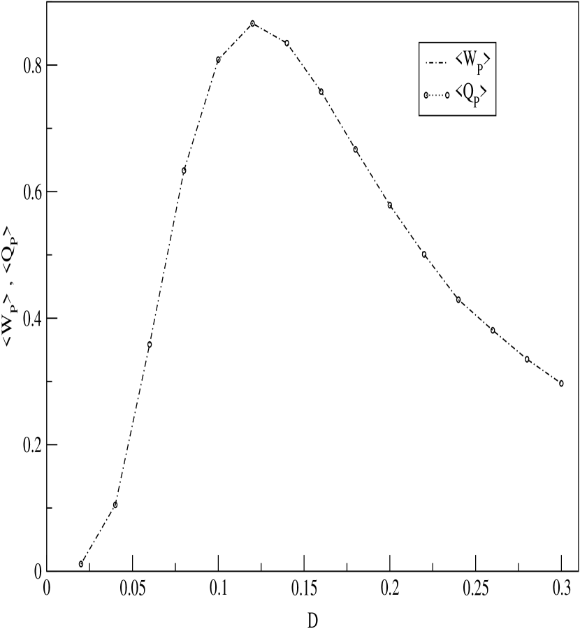
Figure 1:

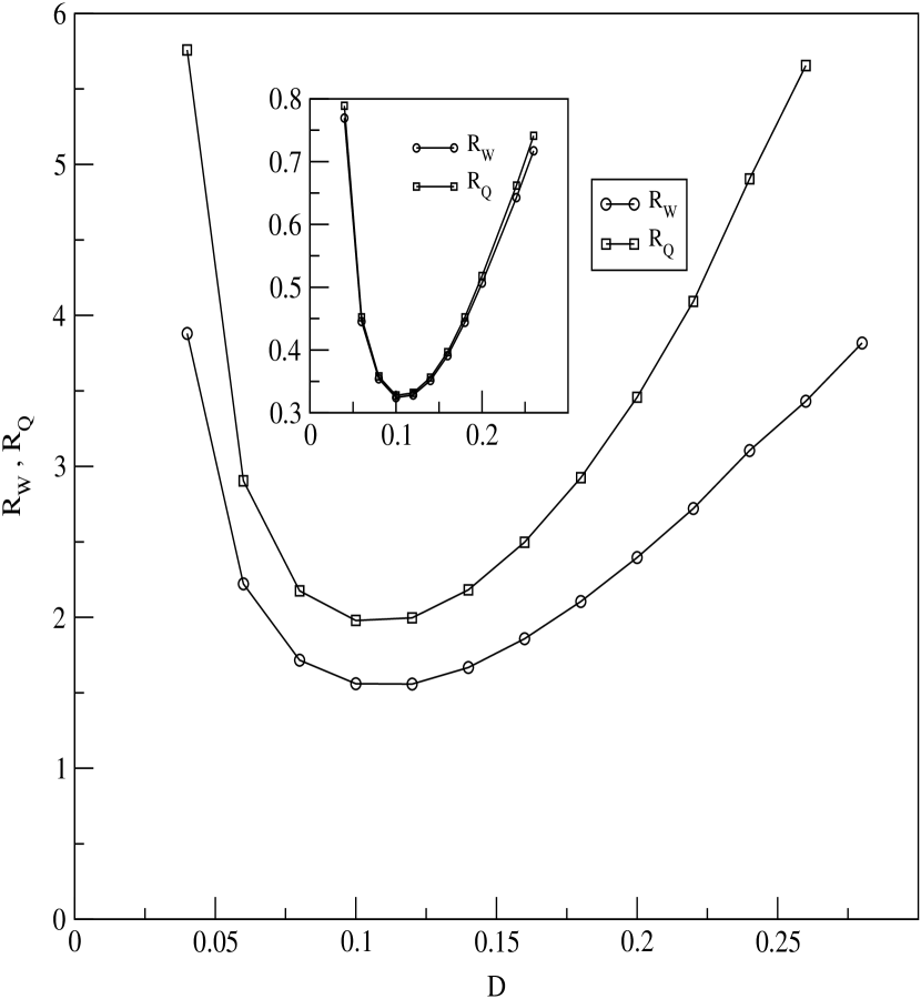
Figure 2:

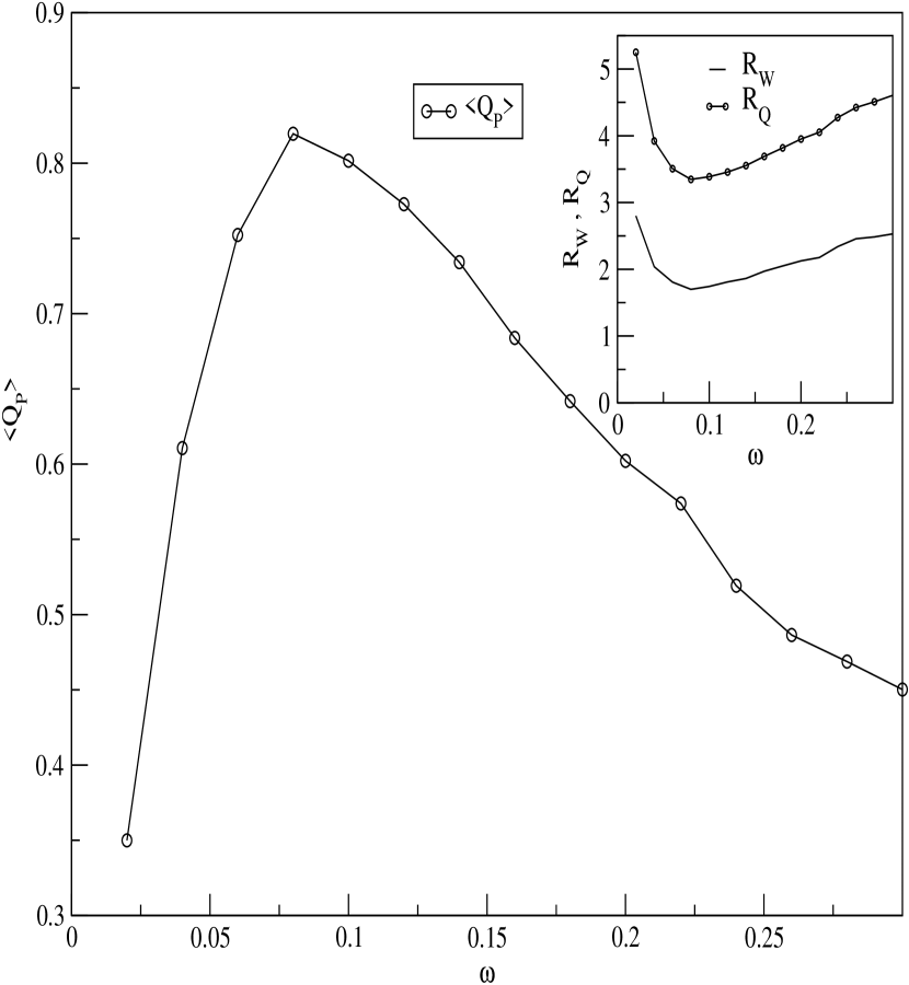
Figure 3:

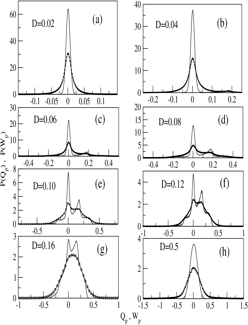
Figure 4:

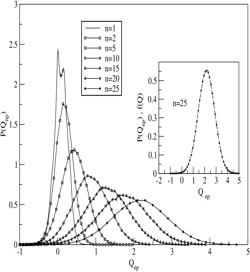
Figure 5:

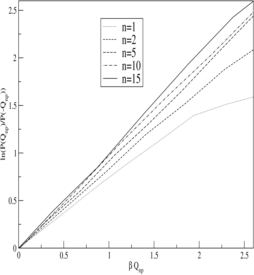
Figure 6:

Figure 7:

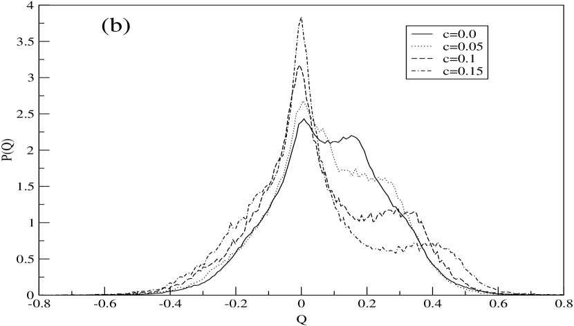
Figure 8:

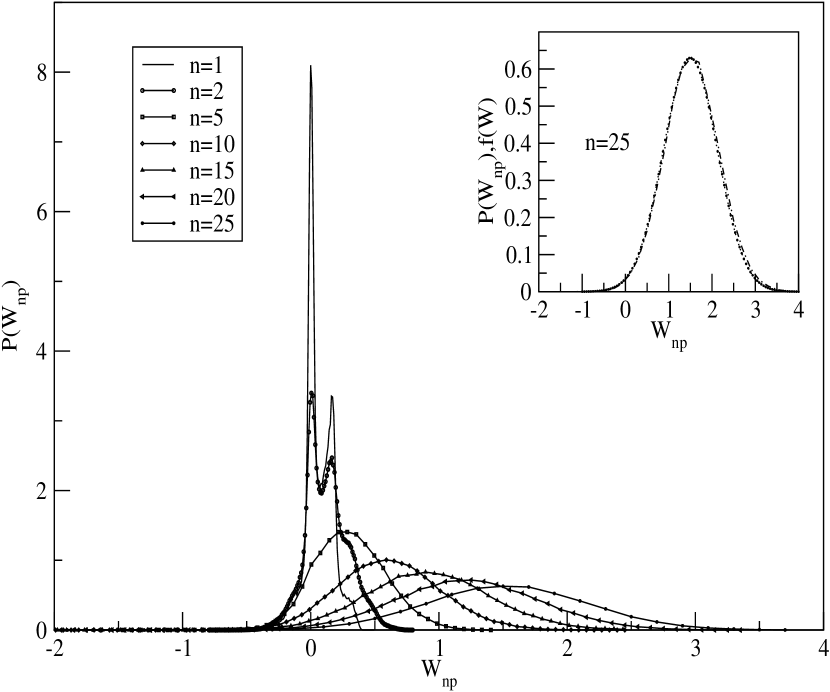
Figure 9:

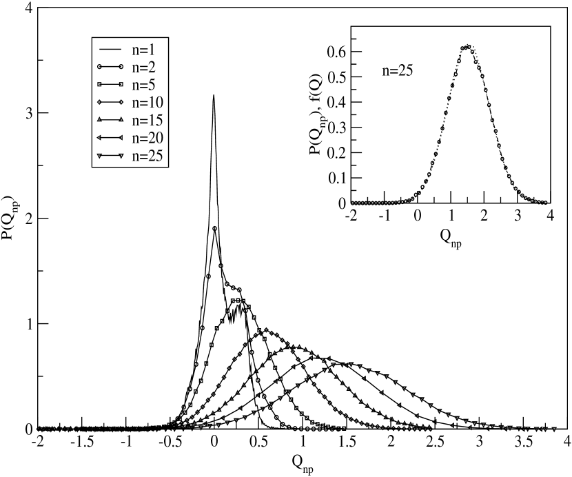
Figure 10:

References

- (1) R. Benzi, G. Parisi, A. Sutera and A. Vulpiani, Tellus 34, (1982) 10.
- (2) L.Gammaitoni, P. Hanggi, P. Jung and F. Marchesoni, Rev. Mod. Phys. 70 (1998) 223.
- (3) T. Wellens, V. Shatokhin and A. Buchleitner, Rep. Prog. Phys. 67 (2005) 45.
- (4) L. Gammaitoni, F. Marchesoni and S. Santucci, Phys. Rev. Lett. 74 (1995) 1052.
- (5) M.H. Choi, R.F. Fox and P. Jung, Phys. Rev. E 57 (1998) 6335.
- (6) G. Giacomelli, F. Marin, and I. Rabbiosi, Phys. Rev. Lett. 82 (1999) 675.
- (7) F. Marchesoni, L. Gammaitoni, F. Apostolico and S. Santucci, Phys. Rev. E 62 (2000) 146.
- (8) M.C. Mahato and S.R. Shenoy, Phys. Rev. E 50 (1994) 2503.
- (9) M.C. Mahato and A.M. Jayannavar, Phys. Rev. E 55 (1997) 6266.
- (10) M.C. Mahato and A.M. Jayannavar, Mod. Phys. Lett. B 11 (1997) 815.
- (11) M.C. Mahato and A.M. Jayannavar, Physica A 248 (1998)138.
- (12) J.C. Phillips and K. Schulten, Phys. Rev. E 52 (1994) 2473.
- (13) M. Thorwart and P. Jung, Phys. Rev. Lett.78 (1997) 2503.
- (14) S.W. Sides, P.A. Rikvold and M.A. Novotny, Phys. Rev. Lett. 81 (1997) 834.
- (15) S.W. Sides, P.A. Rikvold and M.A. Novotny, Phys. Rev. E 57(1998) 6512.
- (16) M. Thorwart, P. Reimann, P. Jung and R.F. Fox, Chem. Phys. 235 (1998) 61.
- (17) J.S. Lim, M.Y. Choi and B.J. Kim, Phys. Rev. B 68 (2003) 012501.
- (18) M. Evstigneev, P. Riemann and C. Bechinger, J.Phys. C 17 (2005) S3795.
- (19) T. Iwai, Physica A 300 (2001) 350.
- (20) T. Iwai, J. Phys. Soc. Jpn. 70 (2001) 353.
- (21) D. Dan and A.M. Jayannavar, Physica A 345 (2005) 404.
- (22) S. Saikia, R. Roy and A.M. Jayannavar, Physics Letters A 369 (2007) 367.
- (23) V. Berdichevsky and M. Gitterman, Physica A 249 (1998) 88.
- (24) C. Bustamante, J. Liphardt and F. Ritort, Physics Today 58 (2005) 45.
- (25) R.J. Harris and G.M. Schültz, J. Stat. Mech. (2007) p07020.
- (26) D. J. Evans and D.J. Searls, Adv. Phys. 51 (2002) 1529.
- (27) C. Jarzynski, Phys. Rev. Lett. 78(1997) 2690.
- (28) C. Jarzynski, Phys. Rev. E 56 (1997) 5018.
- (29) G.E. Crooks, Phys.Rev. E 60 (1999) 2721.
- (30) G.E. Crooks,Phys. Rev. E 61 (2000) 2361.
- (31) F. Hatano and S. Sasa, Phys. Rev. Lett. 86 (2000) 3463.
- (32) W. Lechner et. al, J. Chem. Phys. 124 (2006) 044113.
- (33) G. Hummer and A. Szabo, Proc. Natl. Acad. Sci. 98 (2001) 3658.
- (34) R. van Zon and E.G.D. Cohen, Phys. Rev. E 67 (2002) 046102.
- (35) R. van Zon and E.G.D. Cohen,Phys. Rev. E 69 (2004) 056121.
- (36) O. Mazonka and C. Jarzynski, Cond-mat/ 9912121.
- (37) F. Ritort, J. Stat. Mech. (2004) p10016.
- (38) R.C. Lua and A.Y. Grosberg, J. Phy. Chem. B 109 (2005) 6805.
- (39) L. Bena, C. Van den Broeck and R. Kawai, Europhys. Lett. 71 (2005) 879.
- (40) O. Narayan and A. Dhar, J. Phys. A: Math Gen 37 (2004) 63.
- (41) A. Dhar, Phys. Rev. E 71 (2005) 036126.
- (42) R. Marathe and A. Dhar, Phys. Rev. E 72 (2005) 066112.
- (43) A. Imparato and L. Peliti, Europhys. Lett. 69 (2005) 643.
- (44) A.M. Jayannavar and M. Sahoo, Phys. Rev. E 75, 032102 (2007).
- (45) A. M. Jayannavar and M. Sahoo,cond-mat 0704.2992v1; Pramana J.Phys.(2007) in press.
- (46) A. Saha and A.M. Jayannavar, cond-mat 0707.2131v1.
- (47) J. Liphardt et.al., Science. 296 (2002) 1833.
- (48) F. Douarche et. al., Europhys. Lett. 70 (2005) 593.
- (49) G. M. Wang et. al., Phys. Rev. Lett. 89 (2002).
- (50) E.M. Trepangnier, et. al., Proc. Natl. Acad. Sci. 101 (2004) 15038.
- (51) F. Douarche, S. Joubaud, N.B. Garnier, A. Petrosyan and S. Ciliberto, Phys. Rev. Lett. 97 (2006) 140603.
- (52) R. von Zon, S. Ciliberto and E.G.D. Cohen, Phys. Rev. Lett. 92 (2004) 130601.
- (53) S. Joubaud, N.B. Garnier and S. Ciliberto, cond-mat/0610031.
- (54) H. Risken, The Fokker-Planck Equation, Springer-Verlag, Berlin, 1984.
- (55) K. Sekimoto, J. Phys. Soc. Jpn. 66 (1997)6335.
- (56) R. Mannela, in: J.A. Freund and T. Poschel(Eds), Stochastic Process in Physics, Chemistry and Biology, Lecture Notes in Physics, vol. 557 Springer-Verlag, Berlin (2000) p353.