Magnifying perfect lens and superlens design by coordinate transformation

Abstract

The coordinate transformation technique is applied to the design of perfect lenses and superlenses. In particular, anisotropic metamaterials that magnify two-dimensional planar images beyond the diffraction limit are designed by the use of oblate spheroidal coordinates. The oblate spheroidal perfect lens or superlens can naturally be used in reverse for lithography of planar subwavelength patterns.

I Introduction

Leonhardt leonhardt and Pendry et al. pendry recently suggested an interesting technique of controlling the propagation of electromagnetic fields by the use of metamaterials. In this paper we shall apply this technique to the design of perfect lenses veselago ; pendry_prl ; pendry_oe , which are able to perfectly reproduce an image on another surface, and superlenses pendry_prl ; fang ; melville ; salandrino ; jacob ; liu ; smolyaninov , which apply only to transverse-magnetic (TM) waves. In particular, we show that the technique can be used to design transformation media that magnify images beyond the diffraction limit. Perfect cylindrical lenses have been proposed by Pendry pendry_oe , while cylindrical magnifying superlenses were recently proposed by Salandrino and Engheta salandrino and Jacob et al. jacob and experimentally demonstrated by Liu et al. liu and Smolyaninov et al. smolyaninov . We show that the principle behind such cylindrical devices can be generalized to arbitrary three-dimensional orthogonal coordinate systems. Using the oblate spheroidal coordinates, we further show how perfect lenses and superlenses that magnify planar images with subwavelength features can be designed. The flat object plane is more convenient for imaging and lithography applications.

Our approach yields fundamentally different results from the brief discussion on magnifying perfect lenses in Ref. leonhardt_njp, . We discuss this discrepancy in Section III.2 and argue that the perfect lens design proposed in Ref. leonhardt_njp, does not provide magnification, but rather changes the depth of field or depth of focus only. Our magnifying superlens design, outlined in Sec. V, is also more general and different than that in Ref. salandrino, , in order to avoid the problem of impedance mismatch between the metamaterial with zero transverse permittivity and free space.

II Maxwell Equations under Coordinate Transformation

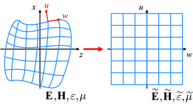
Figure 1: (Color online) Electromagnetic fields $\mathbf{E}$ and $\mathbf{H}$ in a physical medium with material constants $\epsilon$ and $\mu$ can be transformed to normalized fields $\tilde{\mathbf{E}}$ and $\tilde{\mathbf{H}}$ that also obey the Maxwell equations, but regard $(u(x,y,z),v(x,y,z),w(x,y,z))$ as Cartesian coordinates in an effective medium with material constants $\tilde{\epsilon}$ and $\tilde{\mu}$.

For completeness and to establish our notations, we shall first briefly review the invariant property of the Maxwell equations under an orthogonal coordinate transformation moon , closely following Pendry et al. pendry ; ward . The Maxwell equations in terms of harmonic fields in Cartesian coordinates $(x,y,z)$ are

$$\nabla\cdot\left(\epsilon\mathbf{E}\right) =0, \nabla\cdot\left(\mu\mathbf{H}\right) =0,$$

$$\nabla\times\mathbf{E} =i\omega\mu_{0}\mu\mathbf{H}, \nabla\times\mathbf{H} =-i\omega\epsilon_{0}\epsilon\mathbf{E},$$ (1)

where both $\epsilon$ and $\mu$ are second-rank tensors. With a new set of orthogonal coordinates $(u,v,w)$,

$$u =u(x,y,z), v =v(x,y,z), w =w(x,y,z),$$

$$x =x(u,v,w), y =y(u,v,w), z =z(u,v,w),$$ (2)

the fields and the material constants can be rewritten in terms of the new coordinates as

$$\mathbf{E}(u,v,w) \equiv\mathbf{E}\left[x(u,v,w),y(u,v,w),z(u,v,w)\right]$$

$$=\sum_{q=u,v,w}E_{q}(u,v,w)\hat{\mathbf{q}},$$

$$\epsilon(u,v,w) \equiv\epsilon\left[x(u,v,w),y(u,v,w),z(u,v,w)\right]$$

$$=\sum_{p,q}\epsilon_{pq}(u,v,w)\hat{\mathbf{p}}\hat{\mathbf{q}},$$ (3)

and likewise for $\mathbf{H}$ and $\mu$. We assume that $\epsilon$ and $\mu$ are diagonal in the new coordinates, such that

$$\epsilon_{pq} =\epsilon_{q}\delta_{pq}, \mu_{pq} =\mu_{q}\delta_{pq}.$$ (4)

If we define the following normalized fields and material constants,

$$\left(\tilde{E}_{u},\tilde{E}_{v},\tilde{E}_{w}\right) \equiv\left(h_{u}E_{u},h_{v}E_{v},h_{w}E_{w}\right),$$

$$\left(\tilde{H}_{u},\tilde{H}_{v},\tilde{H}_{w}\right) \equiv\left(h_{u}H_{u},h_{v}H_{v},h_{w}H_{w}\right),$$

$$\left(\tilde{\epsilon}_{u},\tilde{\epsilon}_{v},\tilde{\epsilon}_{w}\right) \equiv h_{u}h_{v}h_{w}\left(\frac{\epsilon_{u}}{h_{u}^{2}},\frac{\epsilon_{v}}{h_{v}^{2}},\frac{\epsilon_{w}}{h_{w}^{2}}\right),$$

$$\left(\tilde{\mu}_{u},\tilde{\mu}_{v},\tilde{\mu}_{w}\right) \equiv h_{u}h_{v}h_{w}\left(\frac{\mu_{u}}{h_{u}^{2}},\frac{\mu_{v}}{h_{v}^{2}},\frac{\mu_{w}}{h_{w}^{2}}\right),$$ (5)

where $h_{q}$ is the scale factor of the new coordinates arfken , also called the Lamé coefficients lame ,

$$h_{q}(u,v,w)=\sqrt{\left(\frac{\partial x}{\partial q}\right)^{2}+\left(\frac{\partial y}{\partial q}\right)^{2}+\left(\frac{\partial z}{\partial q}\right)^{2}},$$ (6)

the normalized quantities $\tilde{\mathbf{E}}$, $\tilde{\mathbf{H}}$, $\tilde{\epsilon}$, and $\tilde{\mu}$ satisfy the same Maxwell equations, but now they see $(u,v,w)$ as Cartesian coordinates,

$$\tilde{\nabla}\cdot(\tilde{\epsilon}\tilde{\mathbf{E}}) =0, \tilde{\nabla}\cdot\left(\tilde{\mu}\tilde{\mathbf{H}}\right) =0,$$

$$\tilde{\nabla}\times\tilde{\mathbf{E}} =i\omega\mu_{0}\tilde{\mu}\tilde{\mathbf{H}}, \tilde{\nabla}\times\tilde{\mathbf{H}} =-i\omega\epsilon_{0}\tilde{\epsilon}\tilde{\mathbf{E}},$$ (7)

where

$$\tilde{\nabla} \equiv\hat{\mathbf{u}}\frac{\partial}{\partial u}+\hat{\mathbf{v}}\frac{\partial}{\partial v}+\hat{\mathbf{w}}\frac{\partial}{\partial w}.$$ (8)

In other words, the electromagnetic fields $\mathbf{E}$ and $\mathbf{H}$ in a physical medium with material constants $\epsilon$ and $\mu$ can be transformed to normalized fields $\tilde{\mathbf{E}}$ and $\tilde{\mathbf{H}}$ that also obey the Maxwell equations, but regard $(u(x,y,z),v(x,y,z),w(x,y,z))$ as Cartesian coordinates in an effective medium with material constants $\tilde{\epsilon}$ and $\tilde{\mu}$. See Fig. 1 for an illustration of the coordinate transformation.

III Perfect Lens Design

III.1 General Procedure

In general, a perfect lens should transmit the electromagnetic fields from one surface to another surface with perfect fidelity and without any reflection pendry_prl . Let us define a physical space with a coordinate system $(u^{\prime},v^{\prime},w^{\prime})$ that represent the two surfaces by the equations $w^{\prime}(x^{\prime},y^{\prime},z^{\prime})=a$ and $w^{\prime}(x^{\prime},y^{\prime},z^{\prime})=b$, respectively. If we fill the volume between these two surfaces with metamaterial, an appropriate design of the metamaterial can map the actual fields on these two surfaces onto any other pair of surfaces in a virtual space leonhardt_njp , with another coordinate system $(u,v,w)$, so that the fields propagate in a physical medium with material constants $(\epsilon_{u^{\prime}},\epsilon_{v^{\prime}},\epsilon_{w^{\prime}})$ and $(\mu_{u^{\prime}},\mu_{v^{\prime}},\mu_{w^{\prime}})$ across two surfaces in the physical space as if they propagate across the two mapped surfaces in a virtual medium with $(\epsilon_{u},\epsilon_{v},\epsilon_{w})$ and $(\mu_{u},\mu_{v},\mu_{w})$.

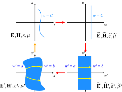
Figure 2: (Color online) The procedure of perfect lens design by the coordinate transformation technique. First a curved surface $w=C$ in the virtual space (top left) is transformed into a plane (top right). The plane is then mapped onto a slab (bottom right), which is subsequently transformed back to the desired geometry in the physical space (bottom left). The electromagnetic fields propagate through the transformation medium with material constants $\epsilon^{\prime}$ and $\mu^{\prime}$ in the physical space as if they propagate within an infinitesimal slab in the virtual space. The fields from a point source on the $w^{\prime}=a$ surface propagate like a ray, depicted by yellow arrows, along a $w^{\prime}$ coordinate line inside the transformation medium.

To make the fields propagate from $w^{\prime}=a$ to $w^{\prime}=b$ without any distortion, one can map the two surfaces in the physical space onto the same surface in the virtual space. A straightforward way is to map all constant-$w^{\prime}$ surfaces within $a\leq w^{\prime}\leq b$ in the physical space onto a single constant-$w$ surface in the virtual space. Mathematically, such a mapping can be achieved if

$$u =u^{\prime}, v =v^{\prime}, w =C, a\leq w^{\prime}\leq b,$$ (9)

where $C$ is an arbitrary constant. The corresponding scale factors are

$$\tilde{h}_{q^{\prime}}\equiv\sqrt{\left(\frac{\partial u}{\partial q^{\prime}}\right)^{2}+\left(\frac{\partial v}{\partial q^{\prime}}\right)^{2}+\left(\frac{\partial w}{\partial q^{\prime}}\right)^{2}}.$$ (10)

The surface mapping function $w=C$ can clearly be generalized to accomodate other requirements. For example, a negative-index material can be used to produce a negative mapping function $w=-w^{\prime}$, so that part of the perfect lens can be free space and the working distance can be increased leonhardt_njp . Nonetheless, in the following we shall use the constant mapping $w=C$ for simplicity. The transformation in the other regions ($w^{\prime}<a,w^{\prime}>b$) can be exploited to simplify the lens design.

To design the metamaterial properties, we should first specify the target virtual material properties $(\epsilon_{u},\epsilon_{v},\epsilon_{w})$ and $(\mu_{u},\mu_{v},\mu_{w})$. For example, if we want the fields to propagate in a virtual free space, we should set $(\epsilon_{u},\epsilon_{v},\epsilon_{w})=(\mu_{u},\mu_{v},\mu_{w})=(1,1,1)$. Next, we transform the fields and material constants in the virtual space to normalized ones,

$$\left(\tilde{E}_{u},\tilde{E}_{v},\tilde{E}_{w}\right) =\left(h_{u}E_{u},h_{v}E_{v},h_{w}E_{w}\right),$$

$$\left(\tilde{H}_{u},\tilde{H}_{v},\tilde{H}_{w}\right) =\left(h_{u}H_{u},h_{v}H_{v},h_{w}H_{w}\right),$$

$$\left(\tilde{\epsilon}_{u},\tilde{\epsilon}_{v},\tilde{\epsilon}_{w}\right) =h_{u}h_{v}h_{w}\left(\frac{\epsilon_{u}}{h_{u}^{2}},\frac{\epsilon_{v}}{h_{v}^{2}},\frac{\epsilon_{w}}{h_{w}^{2}}\right),$$

$$\left(\tilde{\mu}_{u},\tilde{\mu}_{v},\tilde{\mu}_{w}\right) =h_{u}h_{v}h_{w}\left(\frac{\mu_{u}}{h_{u}^{2}},\frac{\mu_{v}}{h_{v}^{2}},\frac{\mu_{w}}{h_{w}^{2}}\right),$$ (11)

so that $(u,v,w)$ become the new Cartesian coordinates in a normalized virtual space. With the coordinate transformation from $(u,v,w)$ to $(u^{\prime},v^{\prime},w^{\prime})$ specified by Eqs. (9) that maps the $w=C$ surface to all constant-$w^{\prime}$ surfaces in the normalized physical space, the normalized quantities become

$$\left(\tilde{E}_{u^{\prime}},\tilde{E}_{v^{\prime}},\tilde{E}_{w^{\prime}}\right) =\left(\tilde{h}_{u^{\prime}}\tilde{E}_{u},\tilde{h}_{v^{\prime}}\tilde{E}_{v},\tilde{h}_{w^{\prime}}\tilde{E}_{w}\right),$$

$$\left(\tilde{H}_{u^{\prime}},\tilde{H}_{v^{\prime}},\tilde{H}_{w^{\prime}}\right) =\left(\tilde{h}_{u^{\prime}}\tilde{H}_{u},\tilde{h}_{v^{\prime}}\tilde{H}_{v},\tilde{h}_{w^{\prime}}\tilde{H}_{w}\right),$$

$$\left(\tilde{\epsilon}_{u^{\prime}},\tilde{\epsilon}_{v^{\prime}},\tilde{\epsilon}_{w^{\prime}}\right) =\tilde{h}_{u^{\prime}}\tilde{h}_{v^{\prime}}\tilde{h}_{w^{\prime}}\left(\frac{\tilde{\epsilon}_{u}}{\tilde{h}_{u^{\prime}}^{2}},\frac{\tilde{\epsilon}_{v}}{\tilde{h}_{v^{\prime}}^{2}},\frac{\tilde{\epsilon}_{w}}{\tilde{h}_{w^{\prime}}^{2}}\right),$$

$$\left(\tilde{\mu}_{u^{\prime}},\tilde{\mu}_{v^{\prime}},\tilde{\mu}_{w^{\prime}}\right) =\tilde{h}_{u^{\prime}}\tilde{h}_{v^{\prime}}\tilde{h}_{w^{\prime}}\left(\frac{\tilde{\mu}_{u}}{\tilde{h}_{u^{\prime}}^{2}},\frac{\tilde{\mu}_{v}}{\tilde{h}_{v^{\prime}}^{2}},\frac{\tilde{\mu}_{w}}{\tilde{h}_{w^{\prime}}^{2}}\right),$$ (12)

Since these new quantities see $(u^{\prime},v^{\prime},w^{\prime})$ as Cartesian coordinates, we should perform the inverse coordinate transform on the normalized quantities, in order to obtain the physical ones that regard $(u^{\prime},v^{\prime},w^{\prime})$ as the desired non-Cartesian coordinate system,

$$\left(E_{u^{\prime}},E_{v^{\prime}},E_{w^{\prime}}\right) =\left(\frac{\tilde{E}_{u^{\prime}}}{h_{u^{\prime}}},\frac{\tilde{E}_{v^{\prime}}}{h_{v^{\prime}}},\frac{\tilde{E}_{w^{\prime}}}{h_{w^{\prime}}}\right),$$

$$\left(H_{u^{\prime}},H_{v^{\prime}},H_{w^{\prime}}\right) =\left(\frac{\tilde{H}_{u^{\prime}}}{h_{u^{\prime}}},\frac{\tilde{H}_{v^{\prime}}}{h_{v^{\prime}}},\frac{\tilde{H}_{w^{\prime}}}{h_{w^{\prime}}}\right),$$

$$\left(\epsilon_{u^{\prime}},\epsilon_{v^{\prime}},\epsilon_{w^{\prime}}\right) =\frac{1}{h_{u^{\prime}}h_{v^{\prime}}h_{w^{\prime}}}\left(h_{u^{\prime}}^{2}\tilde{\epsilon}_{u},h_{v^{\prime}}^{2}\tilde{\epsilon}_{v},h_{w^{\prime}}^{2}\tilde{\epsilon}_{w}\right),$$

$$\left(\mu_{u^{\prime}},\mu_{v^{\prime}},\mu_{w^{\prime}}\right) =\frac{1}{h_{u^{\prime}}h_{v^{\prime}}h_{w^{\prime}}}\left(h_{u^{\prime}}^{2}\tilde{\mu}_{u},h_{v^{\prime}}^{2}\tilde{\mu}_{v},h_{w^{\prime}}^{2}\tilde{\mu}_{w}\right),$$ (13)

where $h_{q^{\prime}}$ is the same scale factor defined in Eq. (6), but with $q^{\prime}=u^{\prime},v^{\prime},w^{\prime}$. As all the constant-$w^{\prime}$ surfaces in the physical space are mapped onto the same surface in the virtual space and thus have identical normalized fields, the fields from a point source on the $w^{\prime}=a$ surface propagate like a ray inside the transformation medium. The rays follow the $w^{\prime}$ coordinate lines, defined as lines along which $u^{\prime}$ and $v^{\prime}$ are constant, much like the rays in an anisotropic metamaterial crystal described by Salandrino and Engheta salandrino . As the coordinate transformation technique is applied to the full Maxwell equations, it also guarantees that waves of arbitrary polarizations can be transmitted perfectly by a perfect lens. Figure 2 depicts the procedure of perfect lens design by the coordinate transformation technique outlined above.

III.2 Planar Perfect Lens

The simplest example is planar imaging with no magnification. One can use Cartesian coordinates for $(u,v,w)$ and $(u^{\prime},v^{\prime},w^{\prime})$ and the following transformation:

$$x =x^{\prime}, y =y^{\prime}, z =\bigg{\{}\begin{array}[]{l}z^{\prime}+b,\\ \delta z^{\prime}+b,\\ z^{\prime}+\delta b\end{array} \begin{array}[]{l}z^{\prime}<0,\\ 0\leq z^{\prime}\leq b,\\ z^{\prime}>b,\end{array}$$ (20)

$$\tilde{h}_{x^{\prime}} =1, \tilde{h}_{y^{\prime}} =1, \tilde{h}_{z^{\prime}} =\bigg{\{}\begin{array}[]{l}1,\\ \delta,\\ 1,\end{array} \begin{array}[]{l}z^{\prime}<0,\\ 0\leq z^{\prime}\leq b,\\ z^{\prime}>b,\end{array}$$ (27)

and let $\delta\to 0$ at the end of the calculation. Assuming that the virtual space is free space, such that $(\epsilon_{x},\epsilon_{y},\epsilon_{z})=(\mu_{x},\mu_{y},\mu_{z})=(1,1,1)$, and using the procedure outlined above, we obtain the following desired physical material constants:

$$\left(\epsilon_{x^{\prime}},\epsilon_{y^{\prime}},\epsilon_{z^{\prime}}\right) =\left(\mu_{x^{\prime}},\mu_{y^{\prime}},\mu_{z^{\prime}}\right)=\Big{\{}\begin{array}[]{l}\left(\delta,\delta,1/\delta\right),\\ \left(1,1,1\right),\end{array} \begin{array}[]{l}0\leq z^{\prime}\leq b,\\ \textrm{otherwise.}\end{array}$$ (32)

The slab is a perfectly matched layer berenger , as one would expect for a reflectionless structure. In the limit of $\delta\to 0$, the fields propagate in the metamaterial slab as if they propagate in an infinitesimal slab at $z=b$ in the virtual free space, so that the fields on one side ($z^{\prime}=0^{-}$) are perfectly transmitted to the other ($z^{\prime}=b^{+}$) without any reflection.

In Ref. leonhardt_njp, , the authors assert that a magnifying perfect lens can be achieved if $\delta$ is negative and different from 1. Their approach yields the following coordinate transformation:

$$x =x^{\prime}, y =y^{\prime}, z =-|\delta|z^{\prime}+C, 0\leq z^{\prime}\leq b.$$ (33)

This coordinate transformation clearly does not provide any magnification, as the transverse coordinates $x$ and $y$ are unchanged, but rather it changes the depth of field or depth of focus only. Instead of producing a magnified perfect image, a misplaced depth of field or depth of focus can only blur the image on the desired image plane, or reproduce a non-magnified perfect image on a different plane.

III.3 Metamaterial Implementation

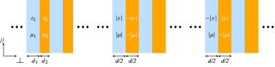
Figure 3: (Color online) Effective anisotropic metamaterial formed by thin films (left), and two possible realizations of the anistropic perfect lens (center and right). The perfect lens can be formed by pairing positive-refractive-index films with negative-refractive-index films of the same thickness (center), as suggested by Veselago veselago and Pendry pendry_prl , or pairing negative-$\epsilon$ films with negative-$\mu$ films (right), as suggested by Alù and Engheta alu .

The highly anisotropic metamaterial specified by Eqs. (32) in the limit of $\delta\to 0$ can be approximately implemented by a stack of thin slabs with alternate signs of permittivity and permeability rytov ; alu ; ramakrishna ; schurig ; tretyakov (Fig. 3). It can be shown, by generalizing the argument in Ref. tretyakov, , that the effective material constants of the stack shown in the left figure of Fig. 3 in the limit of $d_{1}\ll\lambda/|n_{1}|$ and $d_{2}\ll\lambda/|n_{2}|$ are

$$\epsilon_{\parallel} \approx\frac{\epsilon_{1}d_{1}+\epsilon_{2}d_{2}}{d_{1}+d_{2}}, \epsilon_{\perp} \approx\frac{d_{1}+d_{2}}{d_{1}/\epsilon_{1}+d_{2}/\epsilon_{2}},$$

$$\mu_{\parallel} \approx\frac{\mu_{1}d_{1}+\mu_{2}d_{2}}{d_{1}+d_{2}}, \mu_{\perp} \approx\frac{d_{1}+d_{2}}{d_{1}/\mu_{1}+d_{2}/\mu_{2}},$$ (34)

With $\epsilon_{1}=-\epsilon_{2}$ and $\mu_{1}=-\mu_{2}$, the desired anisotropic metamaterial properties are achieved. Two different possible realizations are sketched in the center and right figures of Fig. 3.

We note that the effective medium theory is not exact if the thicknesses of the layers are not significantly smaller than the wavelength tretyakov ; vinogradov . Deviation from Rytov’s effective medium theory of stratified media is an interesting subject that deserves further investigation, but it is beyond the scope of this paper to study this issue, and in the rest of the paper we shall follow the effective medium theory as the first order approximation, which has otherwise withstood theoretical, numerical, and experimental tests salandrino ; jacob ; liu ; smolyaninov ; yariv . Advance in metamaterial technology may also enable new alternative implementations of the desired material parameters.

IV Magnifying Perfect Lenses

IV.1 Spherical Perfect Lens

To achieve magnification, one surface in the physical space, say $w^{\prime}=a$, can be defined to accomodate the object geometry, while the other surface, $w^{\prime}=b$, can be mapped to a larger area, thus converting the fields to far-field radiation for easier detection. The magnifying perfect lens can naturally be used in reverse for lithography. One coordinate system that can achieve magnification is the spherical coordinate system, a natural three-dimensional generalization of the cylindrical geometry studied in Refs. pendry_oe, ; salandrino, ; jacob, ; liu, ; smolyaninov, :

$$x =r\sin\theta\cos\phi, y =r\sin\theta\sin\phi, z =r\cos\theta.$$

$$h_{\theta} =r, h_{\phi} =r\sin\theta, h_{r} =1.$$ (35)

We shall use the following coordinate transformation:

$$\theta =\theta^{\prime}, \phi =\phi^{\prime}, r =\bigg{\{}\begin{array}[]{l}br^{\prime}/a,\\ b,\\ r^{\prime},\end{array} \begin{array}[]{l}r^{\prime}<a,\\ a\leq r^{\prime}\leq b,\\ r^{\prime}>b,\end{array}$$ (42)

$$\tilde{h}_{\theta^{\prime}} =1, \tilde{h}_{\phi^{\prime}} =1, \tilde{h}_{r^{\prime}} =\bigg{\{}\begin{array}[]{l}b/a,\\ 0,\\ 1,\end{array} \begin{array}[]{l}r^{\prime}<a,\\ a\leq r^{\prime}\leq b,\\ r^{\prime}>b,\end{array}$$ (49)

so that all spherical surfaces with $a\leq r^{\prime}\leq b$ are mapped onto a single spherical surface $r=b$ in the virtual space. The coordinate transformation procedure yields

$$\left(\epsilon_{\theta^{\prime}},\epsilon_{\phi^{\prime}},\epsilon_{r^{\prime}}\right) =\frac{b}{a}\left(\epsilon_{\theta},\epsilon_{\phi},\epsilon_{r}\right),$$

$$\left(\mu_{\theta^{\prime}},\mu_{\phi^{\prime}},\mu_{r^{\prime}}\right) =\frac{b}{a}\left(\mu_{\theta},\mu_{\phi},\mu_{r}\right)$$ (50)

for $r^{\prime}<a$,

$$\left(\epsilon_{\theta^{\prime}},\epsilon_{\phi^{\prime}},\epsilon_{r^{\prime}}\right) =\left(\mu_{\theta^{\prime}},\mu_{\phi^{\prime}},\mu_{r^{\prime}}\right)=\left(0,0,\infty\right)$$ (51)

for $a\leq r^{\prime}\leq b$, and

$$\left(\epsilon_{\theta^{\prime}},\epsilon_{\phi^{\prime}},\epsilon_{r^{\prime}}\right) =\left(\mu_{\theta^{\prime}},\mu_{\phi^{\prime}},\mu_{r^{\prime}}\right)=\left(1,1,1\right)$$ (52)

for $r^{\prime}>b$. If we let the virtual space be free space, the desired physical material constants become

$$\left(\epsilon_{\theta^{\prime}},\epsilon_{\phi^{\prime}},\epsilon_{r^{\prime}}\right) =\left(\mu_{\theta^{\prime}},\mu_{\phi^{\prime}},\mu_{r^{\prime}}\right)=\bigg{\{}\begin{array}[]{l}\left(\frac{b}{a},\frac{b}{a},\frac{b}{a}\right),\\ (0,0,\infty),\\ (1,1,1),\end{array} \begin{array}[]{l}r^{\prime}<a,\\ a\leq r^{\prime}\leq b,\\ r^{\prime}>b.\end{array}$$ (59)

The transformation medium consists of an isotropic high-permittivity and high-permeability material for $r^{\prime}<a$, a highly anistropic shell for $a\leq r^{\prime}\leq b$ that can again be implemented by layers of thin spherical shells with alternate signs of permittivity and permeability, and free space for $r^{\prime}>b$. Figure 4 depicts the geometry of the spherical perfect lens, the corresponding virtual space, and the metamaterial implementation.

Figure 4: (Color online) The spherical magnifying perfect lens (center), the corresponding virtual space (left), and the metamaterial implementation of the lens (right). The corresponding regions in the virtual space and the physical space are marked by the same colors in the left and center figures. For clarity, only the $y=0$ cross section is shown. The electromagnetic fields on the inner spherical surface are perfectly mapped onto the outer surface by the lens, enabling far-field detection of subwavelength information. In practice, one can use just half of the spherical lens, so that the object can be placed against the inner spherical surface more conveniently.

The spherical object surface is assumed to be situated at $r^{\prime}=a$, and any electromagnetic fields on the object surface are perfectly transmitted to the outer spherical surface without any reflection. The fields at $r^{\prime}=a^{-}$ are related to the fields at $r^{\prime}=b^{+}$ by

$$\mathbf{E}(\theta^{\prime},\phi^{\prime},b^{+}) =\frac{a}{b}\mathbf{E}(\theta^{\prime},\phi^{\prime},a^{-}),$$

$$\mathbf{H}(\theta^{\prime},\phi^{\prime},b^{+}) =\frac{a}{b}\mathbf{H}(\theta^{\prime},\phi^{\prime},a^{-}).$$ (60)

For large $b$, the fields become primarily far-field radiation at the outer spherical surface that can be detected by conventional far-field optics.

If we make the inner sphere $r^{\prime}<a$ empty for practical reasons, so that $(\epsilon_{\theta^{\prime}},\epsilon_{\phi^{\prime}},\epsilon_{r^{\prime}})=(\mu_{\theta^{\prime}},\mu_{\phi^{\prime}},\mu_{r^{\prime}})=(1,1,1)$ for $r^{\prime}<a$, the fields no longer see the whole virtual space as free space, but as a low-refractive-index sphere with radius $r=b$,

$$\left(\epsilon_{\theta},\epsilon_{\phi},\epsilon_{r}\right) =\left(\mu_{\theta},\mu_{\phi},\mu_{r}\right)=\bigg{\{}\begin{array}[]{l}\left(\frac{a}{b},\frac{a}{b},\frac{a}{b}\right),\\ (1,1,1),\end{array} \begin{array}[]{l}r<b,\\ r\geq b,\end{array}$$ (65)

which can be derived from Eqs. (50). In this case, although the fields on each spherical surface within the metamaterial lens for $a\leq r^{\prime}\leq b$ still have the same azimuthal profiles and are perfectly matched to the outer free space, there is reflection and partial transmission across the inner interface of the metamaterial shell, just as there is reflection and partial transmission across the $r=a$ interface in the virtual space. In other words, there is impedance mismatch between an empty inner volume and the spherical lens, but the image transmission is still perfect. The effects of other deviations from the perfect lens design can also be understood by making more general coordinate transformations and studying the electromagnetic field propagation in the virtual space.

We note that Ref. liu, mentions the possibility of a spherical superlens, while Narimanov’s group at Purdue University also allegedly has unpublished work regarding a spherical superlens, but to our knowledge this is the first time that the specification of a spherical perfect lens and that of a spherical superlens, to be discussed in Sec. V, are reported.

IV.2 Oblate Spheroidal Perfect Lens

The spherical lens is inconvenient for imaging and lithography, as the object or the photoresist must be close to the inner surface of the lens and must therefore also be spherical in shape. To make the object surface flat, the oblate spheroidal coordinate system arfken , illustrated in Fig. 5, is an ideal choice:

$$x =\alpha\cosh w\cos v\cos u,$$

$$y =\alpha\cosh w\cos v\sin u,$$

$$z =\alpha\sinh w\sin v,$$

$$h_{u} =\alpha\cosh w\cos v,$$

$$h_{v} =h_{w}=\alpha\sqrt{\sinh^{2}w+\sin^{2}v}.$$ (66)

Figure 5: (Color online) The oblate spheroidal coordinate system for $0\leq u\leq 3\pi/2$ and $0\leq v\leq\pi/2$. Black lines are coordinate lines, and each color denotes a region between two constant-$w$ surfaces.

We shall use the following transformation to map spheroidal surfaces onto a single one:

$$u =u^{\prime}, v =v^{\prime}, w =\bigg{\{}\begin{array}[]{l}w^{\prime}+b,\\ b,\\ w^{\prime},\end{array} \begin{array}[]{l}0\leq w^{\prime}<a,\\ a\leq w^{\prime}\leq b,\\ w^{\prime}>b,\end{array}$$ (73)

$$\tilde{h}_{u^{\prime}} =1, \tilde{h}_{v^{\prime}} =1, \tilde{h}_{w^{\prime}} =\bigg{\{}\begin{array}[]{l}1,\\ 0,\\ 1,\end{array} \begin{array}[]{l}0\leq w^{\prime}<a,\\ a\leq w^{\prime}\leq b,\\ w^{\prime}>b,\end{array}$$ (80)

and let $a\to 0^{+}$ at the end of the calculation, so that the surface $w^{\prime}=a$ in the physical space becomes flat. Following the coordinate transformation procedure, the desired physical material constants are determined to be

$$(\epsilon_{u^{\prime}},\epsilon_{v^{\prime}},\epsilon_{w^{\prime}}) =\left(\epsilon_{u}\frac{\sinh^{2}b+\sin^{2}v^{\prime}}{\cosh b\sin^{2}v^{\prime}},\epsilon_{v}\cosh b,\epsilon_{w}\cosh b\right),$$

$$(\mu_{u^{\prime}},\mu_{v^{\prime}},\mu_{w^{\prime}}) =\left(\mu_{u}\frac{\sinh^{2}b+\sin^{2}v^{\prime}}{\cosh b\sin^{2}v^{\prime}},\mu_{v}\cosh b,\mu_{w}\cosh b\right)$$ (81)

for $w^{\prime}=0$,

$$(\epsilon_{u^{\prime}},\epsilon_{v^{\prime}},\epsilon_{w^{\prime}}) =(\mu_{u^{\prime}},\mu_{v^{\prime}},\mu_{w^{\prime}})=(0,0,\infty)$$ (82)

for $0<w^{\prime}\leq b$, and

$$(\epsilon_{u^{\prime}},\epsilon_{v^{\prime}},\epsilon_{w^{\prime}}) =(\mu_{u^{\prime}},\mu_{v^{\prime}},\mu_{w^{\prime}})=(1,1,1)$$ (83)

for $w^{\prime}>b$.

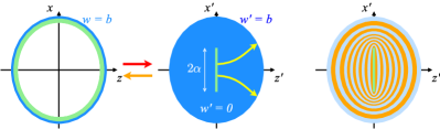
Figure 6: (Color online) Sketches of the oblate spheroidal perfect lens (center), the corresponding virtual space (left), and the metamaterial implementation of the lens (right). For clarity, only the $y^{\prime}=0$ cross sections are drawn. The structure is symmetric with respect to rotation about the $z^{\prime}$ axis. Rays propagate along the $w^{\prime}$ coordinate lines and follow hyperbolic trajectories. In practice, one can use just half of the spheroidal lens ($z^{\prime}>0$) and put the object against the $w^{\prime}=0$ plane.

Figure 6 sketches the geometry of the oblate spheroidal lens. Much like the previous examples, the lens consists of a highly anisotropic material with zero transverse material constants and infinite longitudinal constants, which can be implemented by thin layers of oblate spheroidal films with alternate signs of permittivity and permeability, as shown in Sec. III.3. In this case, the thicknesses of the films, $d_{1}$ and $d_{2}$, should be measured in terms of the $w^{\prime}$ coordinate.

Again, if the material at $w^{\prime}=0$ is made free space for practical reasons, there will be impedance mismatch across the $w^{\prime}=0$ interface between the object plane and the spheroidal lens. Once the fields gets inside the metamaterial, however, the image at the plane $w^{\prime}=0^{+}$ is perfectly magnified and transferred to free space for $w^{\prime}>b$, since the lens and the outer free space are perfectly matched layers.

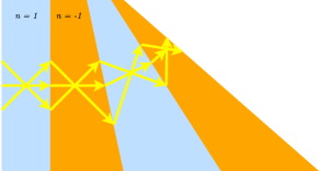
Figure 7: (Color online) A stack of slanted negative-index thin films can continuously redirect a ray with respect to the normal direction of each interface.

An interesting feature of the spheroidal lens is that the $w^{\prime}$ coordinate lines are hyperbolic, so rays inside the transformation medium are also hyperbolic and curved in general. Intuitively, the curved rays can be understood in terms of negative refraction in the ray optics picture, as shown in Fig. 7, if the negative-index thin film implementation is adopted. Negative refraction can focus a point source in free space on the opposite side of the interface pendry_prl ; veselago , so a stack of curved negative-index thin films can continuously redirect a ray with respect to the normal direction of each interface, causing the ray to be curved.

V Superlens Design

The difficulty of controlling permeability without introducing significant loss at optical frequencies has led researchers to the concept of superlens, which has exotic permittivity values but unit permeability and applies only to TM waves pendry_prl ; fang ; melville ; salandrino ; jacob ; liu ; smolyaninov . Because the propagation of TM waves depends not only on the permittivity tensor, but also the transverse permeability, one cannot simply apply the perfect lens specifications on the permittivity only and expect the metamaterial to behave like a perfect lens for TM waves. Instead, it is necessary to examine the TM wave propagation behavior in such a material in order to determine the optimal permittivity values, using the perfect lens design only as a guideline.

To investigate superlensing in more general geometries, let us consider the normalized Maxwell equations in arbitrary orthogonal coordinates, given by Eqs. (7), inside a superlens. Considering TM waves with nonzero $\tilde{H}_{v}$ only,

$$\tilde{E}_{v} =0,$$ (84)

$$\tilde{H}_{u}=\tilde{H}_{w} =0,$$ (85)

$$\frac{\partial\tilde{E}_{u}}{\partial v}=\frac{\partial\tilde{E}_{w}}{\partial v} =0,$$ (86)

$$\frac{\partial}{\partial v}\left(\tilde{\mu}_{v}\tilde{H}_{v}\right) =0,$$ (87)

Eqs. (7) become

$$\frac{\partial\tilde{E}_{u}}{\partial w}-\frac{\partial\tilde{E}_{w}}{\partial u} =i\omega\mu_{0}\tilde{\mu}_{v}\tilde{H}_{v},$$

$$\frac{\partial\tilde{H}_{v}}{\partial w} =i\omega\epsilon_{0}\tilde{\epsilon}_{u}\tilde{E}_{u},$$

$$\frac{\partial\tilde{H}_{v}}{\partial u} =-i\omega\epsilon_{0}\tilde{\epsilon}_{w}\tilde{E}_{w}.$$ (88)

The analysis of TM waves with nonzero $\tilde{H}_{u}$ is similar. The wave equation in terms of $\tilde{H}_{v}$ is

$$\left[\frac{\partial}{\partial w}\left(\frac{1}{\tilde{\epsilon}_{u}}\frac{\partial}{\partial w}\right)+\frac{\partial}{\partial u}\left(\frac{1}{\tilde{\epsilon}_{w}}\frac{\partial}{\partial u}\right)\right]\tilde{H}_{v} =-\frac{\omega^{2}}{c^{2}}\tilde{\mu}_{v}\tilde{H}_{v}.$$ (89)

If we make $\tilde{\epsilon}_{u}=0$ as suggested by Salandrino and Engheta salandrino , the wave equation yields $\partial\tilde{H}_{v}/\partial w=0$, and the normalized magnetic field is uniform with respect to $w$ inside the metamaterial. A point source inside the metamaterial then produces a ray that propagates in the $w$ direction. This phenomenon has been compared salandrino with resonance cones in plasma physics bellan . While such a propagation behavior resembles that in the perfect lenses proposed in the previous sections, the zero transverse permittivity causes significant impedance mismatch between the metamaterial and free space, because resonance cones are well known to be quasi-electrostatic waves and have an infinitesimal magnetic field bellan .

For example, consider the metamaterial slab with zero $\epsilon_{x}$ suggested in Refs. salandrino, ; ramakrishna, (Fig. 8). In the Fourier domain, the wave equation (89) in Cartesian coordinates is

$$\frac{k_{z}^{2}}{\epsilon_{x}}+\frac{k_{x}^{2}}{\epsilon_{z}} =\frac{\omega^{2}}{c^{2}}.$$ (90)

In the limit of $\epsilon_{x}\to 0$, $k_{z}$ is also zero. Equations (88) become

$$-k_{x}E_{z} =\omega\mu_{0}H_{y},$$

$$k_{x}H_{y} =-\omega\epsilon_{0}\epsilon_{z}E_{z},$$ (91)

If we requre $H_{y}$ to be nonzero,

$$E_{z} =-\frac{\omega\mu_{0}}{k_{x}}H_{y}=-\frac{k_{x}}{\omega\epsilon_{0}\epsilon_{z}}H_{y},$$

$$k_{x} =\sqrt{\epsilon_{z}}\frac{\omega}{c}.$$ (92)

Hence the TM wave inside the metamaterial can only have one specific $k_{x}$.

For any other $k_{x}$, $H_{y}$ and $E_{z}$ must vanish, and only $E_{x}$ can be nonzero. In other words, the waves become completely electric and longitudinal, with the electric field parallel to the wave vector. Since the magnetic boundary condition requires the magnetic field to be continuous across the interface between the metamaterial and free space, but the magnetic field of the longitudinal-electric (LE) waves is zero, TM waves in free space cannot be coupled into the LE waves inside the slab and must be completely reflected at the boundary. By reciprocity, the LE waves, once excited inside the slab, also cannot be coupled into free space at all. This means that the planar superlens suggested in Refs. ramakrishna, ; salandrino, is completely unable to transmit an arbitrary TM image in and out of free space. This impedance mismatch problem is especially severe for magnifying superlenses, since one would be unable to observe the magnified image in the far field, while any observed far-field radiation can only be due to imperfections in the metamaterial implementation.

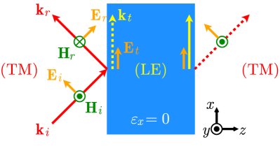
Figure 8: (Color online) TM waves cannot be coupled into a metamaterial slab with zero transverse permittivity, except when the plasmon resonance condition is met, because the TM waves inside the metamaterial are actually LE waves in most cases and have a zero magnetic field. By reciprocity, the LE waves also cannot be coupled into TM waves in free space.

To partially overcome the impedance mismatch problem, it is more desirable to make $\tilde{\epsilon}_{u}$ nonzero and $\tilde{\epsilon}_{w}\to\infty$ instead. The wave equation in terms of $\tilde{H}_{v}$ inside the metamaterial becomes

$$\frac{\partial}{\partial w}\left(\frac{1}{\tilde{\epsilon}_{u}}\frac{\partial\tilde{H}_{v}}{\partial w}\right) =-\frac{\omega^{2}}{c^{2}}\tilde{\mu}_{v}\tilde{H}_{v},$$ (93)

and is independent of the transverse spatial profile of the fields. The other conditions on the fields are

$$\tilde{E}_{w} =0,$$

$$\tilde{E}_{u} =\frac{1}{i\omega\epsilon_{0}\tilde{\epsilon}_{u}}\frac{\partial\tilde{H}_{v}}{\partial w},$$ (94)

resulting in transverse-electric-magnetic (TEM) waves, with a Poynting vector in the $w$ direction regardless of the transverse spatial profile. Crucially, the transverse magnetic field is nonzero as long as $\tilde{\epsilon}_{u}$ is also nonzero, allowing waves inside the metamaterial to be partially coupled to TM waves in free space. The general solution of Eq. (93) is

$$\tilde{H}_{v}(u,v,w)=\tilde{H}_{v}(u,v,a)\tilde{W}_{v}(u,v,w),$$ (95)

where $\tilde{H}_{v}$ must satisfy Eq. (87) and $\tilde{W}_{v}$ is the normalized magnetic field solution for a uniform transverse spatial profile at $w=a$, that is, $\tilde{W}_{v}(u,v,a)=1$ and $\tilde{W}_{v}$ satisfies

$$\frac{\partial}{\partial w}\left(\frac{1}{\tilde{\epsilon}_{u}}\frac{\partial\tilde{W}_{v}}{\partial w}\right) =-\frac{\omega^{2}}{c^{2}}\tilde{\mu}_{v}\tilde{W}_{v}.$$ (96)

The boundary spatial profile $\tilde{H}_{v}(u,v,a)$ acts as a spatial modulation of the field throughout propagation and does not diffract, even though $\tilde{W}_{v}$ may change its shape along $w$. Thus, an arbitrary TM image can be carried as a modulation of $\tilde{W}_{v}$ from one surface to another without loss of information. For lithography, the boundary spatial profile is applied at $w=b$, and the converging wave solution of Eq. (96) should be used instead.

For instance, for a planar superlens with $\epsilon_{z}\to\infty$, we obtain

$$H_{y}(x,z) =H_{y}(x,0)\exp\left(i\sqrt{\epsilon_{x}}\frac{\omega}{c}z\right),$$

$$H_{x}(y,z) =H_{x}(y,0)\exp\left(i\sqrt{\epsilon_{y}}\frac{\omega}{c}z\right).$$ (97)

$k_{z}$ is constant, and a TM image can be perfectly transmitted inside the lens, apart from an unimportant phase factor. Using the approximate effective medium theory outlined in Sec. III.3,

$$\frac{d_{1}}{\epsilon_{1}}+\frac{d_{2}}{\epsilon_{2}} =0,$$

$$\epsilon_{z} \approx\infty,$$

$$\epsilon_{x}=\epsilon_{y} \approx\epsilon_{1}+\epsilon_{2}.$$ (98)

To make the waves propagating, $\epsilon_{x}$ and $\epsilon_{y}$ must be positive.

Depending on loss and other limitations in the metamaterial implementation, such as finite thicknesses of the thin films, $\tilde{\epsilon}_{w}$ obviously cannot be infinite in practice. In the planar geometry, assuming $k_{y}=0$ for simplicity, $k_{z}$ becomes

$$k_{z} =\sqrt{\epsilon_{x}}\sqrt{\frac{\omega^{2}}{c^{2}}-\frac{k_{x}^{2}}{\epsilon_{z}}}$$

$$=\sqrt{\epsilon_{x}}\frac{\omega}{c}\left[1-\frac{1}{\epsilon_{z}}\left(\frac{k_{x}\lambda}{2\pi}\right)^{2}\right]^{1/2},$$ (99)

where $\lambda$ is the free-space wavelength. The Abbe limit for the superlens is therefore roughly given by

$$\Delta_{\textrm{min}}\sim\frac{\lambda}{2\sqrt{|\epsilon_{z}|}}.$$ (100)

The resolution limit depends directly on the magnitude of the longitudinal refractive index $\sqrt{|\epsilon_{z}|}$.

Let us estimate the resolution limit at $\lambda=365$ nm due to loss in a stack of infinitesimally thin silver ($\epsilon_{1}\approx-2.4+0.25i$) and aluminium oxide ($\epsilon_{2}\approx 3.2$) layers. Using the approximate effective medium theory, the maximum longitudinal index $\sqrt{|\epsilon_{z}|}$ is about 7.4, at a $d_{1}/d_{2}$ ratio of $0.75$. This means that the free-space resolution limit can be beaten by roughly a factor of 7. To obtain a more accurate assessment of the resolution limit and that in other geometries, more numerical and experimental studies are needed.

The $\epsilon_{w}\to\infty$ condition can naturally be applied to magnifying configurations. For spherical coordinates, the physical solution of Eq. (93) is the spherical wave,

$$H_{\phi}(\theta,r) =H_{\phi}(\theta,a)\frac{a}{r}\exp\left[i\sqrt{\epsilon_{\theta}}\frac{\omega}{c}(r-a)\right],$$

$$H_{\theta}(\phi,r) =H_{\theta}(\phi,a)\frac{a}{r}\exp\left[i\sqrt{\epsilon_{\phi}}\frac{\omega}{c}(r-a)\right].$$ (101)

For oblate spheroidal coordinates, the spheroidal wave functions are much more complicated and given by

$$\quad\frac{\partial}{\partial w}\left\{\frac{\cosh w}{\sinh^{2}w+\sin^{2}v}\frac{\partial}{\partial w}\left[\sqrt{\sinh^{2}w+\sin^{2}v}H_{v}(u,v,w)\right]\right\}$$

$$=-\frac{\omega^{2}}{c^{2}}\alpha^{2}\epsilon_{u}\cosh w\sqrt{\sinh^{2}w+\sin^{2}v}H_{v}(u,v,w),$$

$$\quad\frac{\partial}{\partial w}\left\{\frac{1}{\cosh w}\frac{\partial}{\partial w}\left[\cosh wH_{u}(v,w)\right]\right\}$$

$$=-\frac{\omega^{2}}{c^{2}}\alpha^{2}\epsilon_{v}\left(\sinh^{2}w+\sin^{2}v\right)H_{u}(v,w).$$ (102)

but arbitrary TM images can still be transmitted as transverse spatial modulations of the spheroidal wave functions.

In the limit of high magnification, TM waves in free space become approximately TEM waves, so the TEM waves inside the magnifying superlenses can be efficiently coupled to free space, if $\epsilon_{u}$ is close to $1$.

VI Conclusion

In conclusion, we have outlined the procedure of magnifying perfect lens and superlens design by the coordinate transformation technique. The use of oblate spheroidal coordinates is especially promising for subwavelength microscopy and lithography, as they provide a more convenient flat object or image plane and enable two-dimensional magnification beyond the diffraction limit. For a simpler experimental setup, the elliptic cylindrical coordinates arfken can also be used to provide a flat object plane and one-dimensional magnification. Given the recent success in superlens experiments, the oblate spheroidal or elliptic cylindrical superlens should be relatively straightforward to demonstrate experimentally. Loss is a major problem, and more theoretical, numerical, and experimental analysis is needed to evaluate the impact of loss and other deviations from the ideal design in practice. In applications where a strong signal is preferred and loss in metamaterials is a major detrimental factor, resonantly-enhanced near-field imaging by low-loss dielectric structures may be a better option tsang .

References

- (1) U. Leonhardt, Science 312, 1777 (2006).
- (2) J. B. Pendry, D. Schurig, and D. R. Smith, Science 312, 1780 (2006).
- (3) V. G. Veselago, Sov. Phys. Usp. 10, 509 (1968).
- (4) J. B. Pendry, Phys. Rev. Lett. 85, 3966 (2000).
- (5) J. B. Pendry, Opt. Express 11, 755 (2003).
- (6) N. Fang, H. Lee, C. Sun, and X. Zhang, Science 308, 534 (2005).
- (7) D. O. S. Melville and R. J. Blaikie, Opt. Express 13, 2127 (2005).
- (8) A. Salandrino and N. Engheta, Phys. Rev. B74, 075103 (2006).
- (9) Z. Jacob, L. V. Alekseyev, and E. Narimanov, Opt. Express 14, 8247 (2006).
- (10) Z. Liu, H. Lee, Y. Xiong, C. Sun, and X. Zhang, Science 315, 1686 (2007).
- (11) I. I. Smolyaninov, Y.-J. Hung, and C. C. Davis, Science 315, 1699 (2007).
- (12) U. Leonhardt and T. G. Philbin, New J. Phys. 8, 247 (2006).
- (13) P. H. Moon and D. E. Spencer, Field Theory Handbook (Springer-Verlag, Berlin, 1961); A. Alù, F. Bilotti, and L. Vegni, IEEE Tran. Antennas Propagat. 52, 1530 (2004); and references therein.
- (14) A. J. Ward and J. B. Pendry, J. Mod. Opt. 43, 773 (1996).
- (15) G. Arfken, Mathematical Methods for Physicists (Academic Press, Orlando, 1970).
- (16) G. Lamé, Leçons sur les Coordonnés Curvilignes et Leurs Diverses Applications (Mallet-Bachelier, Paris, 1859).
- (17) J.-P. Berenger, J. Comput. Phys. 114, 185 (1994).
- (18) S. M. Rytov, Sov. Phys. JETP 2, 466 (1956).
- (19) A. Alù and N. Engheta, IEEE Tran. Antennas Propagat. 51, 2558 (2003).
- (20) S. A. Ramakrishna, J. B. Pendry, M. C. K. Wiltshire, and W. J. Stewart, J. Mod. Opt. 50, 1419 (2003).
- (21) D. Schurig and D. R. Smith, New J. Phys. 7, 162 (2005).
- (22) S. Tretyakov, “Composite materials,” in Analytical Modeling in Applied Electromagnetics (Artech House, Norwood, 2000), pp. 119-192.
- (23) A. P. Vinogradov and A. M. Merzlikin, Doklady Phys. 46, 832 (2001); A. P. Vinogradov and A. M. Merzlikin, J. Exp. Theor. Phys. 94, 482 (2002); D. R. Smith and J. B. Pendry, J. Opt. Soc. Am. B23, 391 (2006); C. R. Simovski and S. A. Tretyakov, Phys. Rev. B75, 195111 (2007).
- (24) J. P. van der Ziel, M. Ilegems, and R. M. Mikulyak, Appl. Phys. Lett. 28, 735 (1976); P. Yeh, A. Yariv, and C.-S. Hong, J. Opt. Soc. Am. 67, 423 (1977); A. Yariv and P. Yeh, J. Opt. Soc. Am. 67, 423 (1977); R. C. McPhedran, L. C. Botten, M. S. Craig, M. Nevière, and D. Maystre, J. Mod. Opt. 29, 289 (1982); P. Lalanne and D. Lemercier-Lalanne, J. Mod. Opt. 43, 2063 (1996); and references therein.
- (25) P. M. Bellan, “Cold plasma waves in a magnetized plasma,” in Fundamentals of Plasma Physics (Cambridge University Press, Cambridge, 2006), pp. 206-240.
- (26) M. Tsang and D. Psaltis, Opt. Lett. 31, 2741 (2006); 32, 86 (2007); M. Tsang and D. Psaltis, Opt. Express 15, 11959 (2007).