HIGH ENERGY SCATTERING
IN QUANTUM
CHROMODYNAMICS111Lectures given at the Xth
Hadron Physics Workshop, March 2007, Florianopolis, Brazil.
Abstract
In this series of three lectures, we discuss several aspects of high energy scattering among hadrons in Quantum Chromodynamics. The first lecture is devoted to a description of the parton model, Bjorken scaling and the scaling violations due to the evolution of parton distributions with the transverse resolution scale. The second lecture describes parton evolution at small momentum fraction , the phenomenon of gluon saturation and the Color Glass Condensate (CGC). In the third lecture, we present the application of the CGC to the study of high energy hadronic collisions, with emphasis on nucleus-nucleus collisions. In particular, we provide the outline of a proof of high energy factorization for inclusive gluon production.
Preprint CERN-PH-TH/2007-131
1 Introduction
Quantum Chromodynamics (QCD) is very successful at describing hadronic scatterings involving very large momentum transfers. A crucial element in these successes is the asymptotic freedom of QCD [1], that renders the coupling weaker as the momentum transfer scale increases, thereby making perturbation theory more and more accurate. The other important property of QCD when comparing key theoretical predictions to experimental measurements is the factorization of the short distance physics which can be computed reliably in perturbation theory from the long distance strong coupling physics related to confinement. The latter are organized into non-perturbative parton distributions, that depend on the scales of time and transverse space at which the hadron is resolved in the process under consideration. In fact, QCD not only enables one to compute the perturbative hard cross-section, but also predicts the scale dependence of the parton distributions.
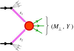
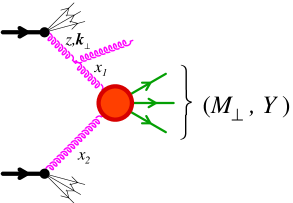
A generic issue in the application of perturbative QCD to the study of hadronic scatterings is the occurrence of logarithmic corrections in higher orders of the perturbative expansion. These logarithms can be large enough to compensate the extra coupling constant they come accompanied with, thus voiding the naive, fixed order, application of perturbation theory. Consider for instance a generic gluon-gluon fusion process, as illustrated on the left of figure 1, producing a final state of momentum . The two gluons have longitudinal momentum fractions given by
| (1) |
where ( is the invariant mass of the final state) and . On the right of figure 1 is represented a radiative correction to this process, where a gluon is emitted from one of the incoming lines. Roughly speaking, such a correction is accompanied by a factor
| (2) |
where is the momentum fraction of the gluon before the splitting, and its transverse momentum. Such corrections produce logarithms, and , that respectively become large when is small or when is large compared to typical hadronic mass scales. These logarithms tell us that parton distributions must depend on the momentum fraction and on a transverse resolution scale , that are set by the process under consideration. In the linear regime222We use the denomination “linear” here to distinguish it from the saturation regime discussed later that is characterized by non-linear evolution equations., there are “factorization theorems” – -factorization [2] in the first case and collinear factorization [3] in the second case – that tell us that the logarithms are universal and can be systematically absorbed in the definition of parton distributions 333The latter is currently more rigorously established than the former.. The dependence that results from resumming the logarithms of is taken into account by the BFKL equation [4]. Similarly, the dependence on the transverse resolution scale is accounted for by the DGLAP equation [5].
The application of QCD is a lot less straightforward for scattering at very large center of mass energy, and moderate momentum transfers. This kinematics in fact dominates the bulk of the cross-section at collider energies. A striking example of this kinematics is encountered in Heavy Ion Collisions (HIC), when one attempts to calculate the multiplicity of produced particles. There, despite the very large center of mass energy444At RHIC, center of mass energies range up to GeV/nucleon; the LHC will collide nuclei at TeV/nucleon., typical momentum transfers are small555For instance, in a collision at GeV between gold nuclei at RHIC, 99% of the multiplicity comes from hadrons whose is below 2 GeV., of the order of a few GeVs at most. In this kinematics, two phenomena that become dominant are
-
•
Gluon saturation : the linear evolution equations (DGLAP or BFKL) for the parton distributions implicitly assume that the parton densities in the hadron are small and that the only important processes are splittings. However, at low values of , the gluon density may become so large that gluon recombinations are an important effect.
-
•
Multiple scatterings : processes involving more than one parton from a given projectile become sizeable.
It is highly non trivial that this dominant regime of hadronic interactions is amenable to a controlled perturbative treatment within QCD, and the realization of this possibility is a major theoretical advance in the last decade. The goal of these three lectures is to present the framework in which such calculations can be carried out.
In the first lecture, we will review key aspects of the parton model. Our recurring example will be the Deep Inelastic Scattering (DIS) process of scattering a high energy electron at high momentum transfers off a proton. Beginning with the inclusive DIS cross-section, we will arrive at the parton model (firstly in its most naive incarnation, and then within QCD), and subsequently at the DGLAP evolution equations that control the scaling violations measured experimentally.
In the second lecture, we will address the evolution of the parton model to small values of the momentum fraction and the saturation of the gluon distribution. After illustrating the tremendous simplification of high energy scattering in the eikonal limit, we will derive the BFKL equation and its non-linear extension, the BK equation. We then discuss how these evolution equations arise in the Color Glass Condensate effective theory. We conclude the lecture with a discussion of the close analogy between the energy dependence of scattering amplitudes in QCD and the temporal evolution of reaction-diffusion processes in statistical mechanics.
The third lecture is devoted to the study of nucleus-nucleus collisions at high energy. Our main focus is the study of bulk particle production in these reactions within the CGC framework. After an exposition of the power counting rules in the saturated regime, we explain how to keep track of the infinite sets of diagrams that contribute to the inclusive gluon spectrum. Specifically, we demonstrate how these can be resummed at leading and next-to-leading order by solving classical equations of motion for the gauge fields The inclusive quark spectrum is discussed as well. We conclude the lecture with a discussion of the inclusive gluon spectrum at next-to-leading order and outline a proof of high energy factorization in this context. Understanding this factorization may hold the key to understanding early thermalization in heavy ion collisions. Some recent progress in this direction is briefly discussed.
2 Lecture I : Parton model, Bjorken scaling, scaling violations
In this lecture, we will begin with the simple parton model and develop the conventional Operator Product Expansion (OPE) approach and the associated DGLAP evolution equations. To keep things as simple as possible, we will use Deep Inelastic Scattering to illustrate the ideas in this lecture.
2.1 Kinematics of DIS
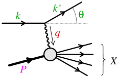
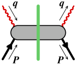
The basic idea of Deep Inelastic Scattering (DIS) is to use a well understood lepton probe (that does not involve strong interactions) to study a hadron. The interaction is via the exchange of a virtual photon666If the virtuality of the photon is small (in photo-production reactions for instance), the assertion that the photon is a “well known probe that does not involve strong interactions” is not valid anymore. Indeed, the photon may fluctuate, for instance, into a meson.. Variants of this reaction involve the exchange of a or boson which become increasingly important at large momentum transfers. The kinematics of DIS is characterized by a few Lorentz invariants (see figure 2 for the notations), traditionally defined as
| (3) |
where is the nucleon mass (assuming that the target is a proton) and the invariant mass of the hadronic final state. Because the exchanged photon is space-like, one usually introduces , and also . Note that since , we must have – the value being reached only in the case where the proton is scattered elastically.
The simplest cross-section one can measure in a DIS experiment is the total inclusive electron+proton cross-section, where one sums over all possible hadronic final states :
| (4) |
The partial cross-section associated to a given final state can be written as
| (5) |
where denotes the invariant phase-space element for the final state and is the corresponding transition amplitude. The “spin” symbol denotes an average over all spin polarizations of the initial state and a sum over those in the final state. The transition amplitude is decomposed into an electromagnetic part and a hadronic matrix element as
| (6) |
In this equation is the hadron electromagnetic current that couples to the photon, and denotes a state containing a nucleon of momentum .
Squaring this amplitude and collecting all the factors, the inclusive DIS cross-section can be expressed as
| (7) |
where the leptonic tensor (neglecting the electron mass) is
| (8) | |||||
and – the hadronic tensor – is defined as
| (9) | |||||
The second equality is obtained using the complete basis of hadronic states . Thus, the hadronic tensor is the Fourier transform of the expectation value of the product of two currents in the nucleon state. An important point is that this object cannot be calculated by perturbative methods. This rank-2 tensor can be expressed simply in terms of two independent structure functions as a consequence of
-
•
Conservation of the electromagnetic current :
-
•
Parity and time-reversal symmetry :
-
•
Electromagnetic currents conserve parity : the Levi-Civita tensor cannot appear777This property is not true in DIS reactions involving the exchange of a weak current; an additional structure function is needed in this case. in the tensorial decomposition of
When one works out these constraints, the most general tensor one can construct from and reads :
| (10) |
where are the two structure functions888The structure function differs slightly from the defined in [6] : .. As scalars, they only depend on Lorentz invariants, namely, the variables and . The inclusive DIS cross-section in the rest frame of the proton can be expressed in terms of as
| (11) |
where represents the solid angle of the scattered electron and its energy.
2.2 Experimental facts
Two major experimental results from SLAC [7] in the late 1960’s played a crucial role in the development of the parton model.
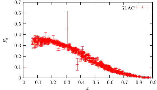
The left plot of figure 3 shows the measured values of as a function of . Even though the data covers a significant range in , all the data points seem to line up on a single curve, indicating that depends very little on in this regime. This property is now known as Bjorken scaling [8]. In the right plot of figure 3, one sees a comparison of with the combination999, the longitudinal structure function, describes the inclusive cross-section between the proton and a longitudinally polarized proton. . Although there are few data points for , one can see that it is significantly lower than and close to zero 101010From current algebra, it was predicted that ; this relation is known as the Callan-Gross relation [9].. As we shall see shortly, these two experimental facts already tell us a lot about the internal structure of the proton.
2.3 Naive parton model
In order to get a first insight into the inner structure of the proton, it is interesting to compare the DIS cross-section in eq. (11) and the cross-section (also expressed in the rest frame of the muon),
| (12) |
Note that, since this reaction is elastic, the corresponding variable is equal to , hence the delta function in the prefactor. The comparison of this formula with eq. (11), and in particular its angular dependence, is suggestive of the proton being composed of point like fermions – named partons by Feynman – off which the virtual photon scatters. If the constituent struck by the photon carries the momentum , this comparison suggests that
| (13) |
Assuming that this parton carries the fraction of the momentum of the proton, i.e. , the relation between the variables and is . Therefore, we get :
| (14) |
In other words, the kinematical variable measured from the scattering angle of the electron would be equal to the fraction of momentum carried by the struck constituent. Note that Bjorken scaling appears quite naturally in this picture.
Having gained intuition into what may constitute a proton, we shall now compute the hadronic tensor for the DIS reaction on a free fermion carrying the fraction of the proton momentum. Because we ignore interactions for the time being, this calculation (in contrast to that for a proton target) can be done in closed form. We obtain,
where is the electric charge of the parton under consideration. Let us now assume that in a proton there are partons of type with a momentum fraction between and , and that the photon scatters incoherently off each of them. We would thus have
| (15) |
(The factor in the denominator is a “flux factor”.) At this point, we can simply read the values of ,
| (16) |
We thus see that the two experimental observations of i) Bjorken scaling and ii) the Callan-Gross relation are automatically realized in this naive picture of the proton111111In particular, in this model is intimately related to the spin structure of the scattered partons. Scalar partons, for instance, would give , at variance with experimental results..
Despite its success, this model is quite puzzling, because it assumes that partons are free inside the proton – while the rather large mass of the proton suggests a strong binding of these constituents inside the proton. Our task for the rest of this lecture is to study DIS in a quantum field theory of strong interactions, thereby turning the naive parton model into a systematic description of hadronic reactions. Before we proceed further, let us describe in qualitative terms (see [10] for instance) what a proton constituted of fermionic constituents bound by interactions involving the exchange of gauge bosons may look like.
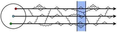
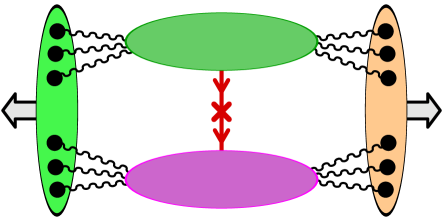
In the left panel of figure 4 are represented the three valence partons (quarks) of the proton. These quarks interact by gluon exchanges, and can also fluctuate into states that contain additional gluons (and also quark-antiquark pairs). These fluctuations can exist at any space-time scale smaller than the proton size ( 1 fermi). (In this picture, one should think of the horizontal axis as the time axis.) When one probes the proton in a scattering experiment, the probe (e.g. the virtual photon in DIS) is characterized by certain resolutions in time and in transverse coordinate. The shaded area in the picture is meant to represent the time resolution of the probe : any fluctuation which is shorter lived than this resolution cannot be seen by the probe, because it appears and dies out too quickly.
In the right panel of figure 4, the same proton is represented after a boost, while the probe has not changed. The main difference is that all the internal time scales are Lorentz dilated. As a consequence, the interactions among the quarks now take place over times much larger than the resolution of the probe. The probe therefore sees only free constituents. Moreover, this time dilation allows more fluctuations to be resolved by the probe; thus, a high energy proton appears to contain more gluons than a proton at low energy121212Equivalently, if the energy of the proton is fixed, there are more gluons at lower values of the momentum fraction ..
2.4 Bjorken scaling from free field theory
We will now derive Bjorken scaling and the Callan-Gross relation from quantum field theory. We will consider a theory involving fermions (quarks) and bosons (gluons), but shall at first consider the free field theory limit by neglecting all their interactions. We will consider a kinematical regime in DIS that involves a large value of the momentum transfer and of the center of mass energy of the collision, while the value of is kept constant. This limit is known as the Bjorken limit.
To appreciate strong interaction physics in the Bjorken limit, consider a frame in which the 4-momentum of the photon can be written as
| (17) |
From the combinations of the components of
| (18) |
and because , the integration over in is dominated by
| (19) |
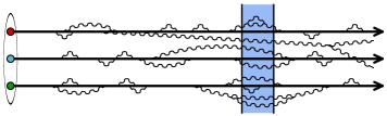
Therefore, the invariant separation between the points at which the two currents are evaluated is . Noting that in eq. (9) the product of the two currents can be replaced by their commutator, and recalling that expectation values of commutators vanish for space-like separations, we also see that . Thus, the Bjorken limit corresponds to a time-like separation between the two currents, with the invariant separation going to zero, as illustrated in figure 5.
It is important to note that in this limit, although the invariant goes to zero, the components of do not necessarily become small. This will have important ramifications when we apply the Operator Product Expansion to .
For our forthcoming discussion, consider the forward Compton amplitude
| (20) |
It differs from by the fact that the two currents are time-ordered, and as illustrated in figure 6, one can recover from its imaginary part,
| (21) |
At fixed , is analytic in the variable , except for two cuts on the real axis that start at . The cut at positive corresponds to the threshold above which the DIS reaction becomes possible, and the cut at negative can be inferred from the fact that is unchanged under the exchange . It is also possible to decompose the tensor in terms of two structure functions :
| (22) |
and the DIS structure functions can be expressed in terms of the discontinuity of across the cuts.
We now remind the reader of some basic results about the Operator Product Expansion (OPE) [11, 12]. Consider a correlator , where and are two local operators (possibly composite) and the ’s are unspecified field operators. In the limit , this object is usually singular, because products of operators evaluated at the same point are ill-defined. The OPE states that the nature of these singularities is a property of the operators and , and is not influenced by the nature and localization of the ’s. This singular behavior can be expressed as
| (23) |
where the are numbers (known as the Wilson coefficients) that contain the singular dependence and the are local operators that have the same quantum numbers as the product . This expansion – known as the OPE – can then be used to obtain the limit of any correlator containing the product . If ,and are the respective mass dimensions of the operators and , a simple dimensional argument tells us that
| (24) |
(Here .) From this relation, we see that the operators having the lowest dimension lead to the most singular behavior in the limit . Thus, only a small number of operators are relevant in the analysis of this limit and one can ignore the higher dimensional operators.
Things are however a bit more complicated in the case of DIS, because only the invariant goes to zero, while the components do not go to zero. The local operators that may appear in the OPE of can be classified according to the representation of the Lorentz group to which they belong. Let us denote them , where is the “spin” of the operator (the number of Lorentz indices it carries), and the index labels the various operators having the same Lorentz structure. The OPE can be written as :
| (25) |
Because they depend only on the 4-vector , the Wilson coefficients must be of the form131313There could also be terms where one or more pairs are replaced by , but such terms are less singulars in the Bjorken limit.
| (26) |
where depends only on the invariant . Similarly, the expectation value of the operators in the proton state can only depend on the proton momentum , and the leading part in the Bjorken limit is141414Here also, there could be terms where a pair is replaced by , but they too lead to subleading contributions in the Bjorken limit.
| (27) |
where the are some non-perturbative matrix elements.
Let us now denote by the mass dimension of the operator . Then, the dimension of is , which means that it scales like
| (28) |
Because the individual components of do not go to zero, it is this scaling alone that determines the behavior of the hadronic tensor in the Bjorken limit. Contrary to the standard OPE, the scaling depends on the difference between the dimension of the operator and its spin, called its twist , rather than its dimension alone. The Bjorken limit of DIS is dominated by the operators that have the lowest possible twist. As we shall see, there is an infinity of these lowest twist operators, because the dimension can be compensated by the spin of the operator. If we go back to the structure functions , we can write
| (29) |
where and . The difference by one power of (at fixed ) between and comes from their respective definitions from that differ by one power of the proton momentum . Eq. (29) gives the structure functions as a series of terms, each of which has factorized and dependences. (The functions () are related to the Fourier transform of , and thus can only depend on the invariant ). Moreover, for dimensional reasons, the functions must scale like . Therefore, it follows that Bjorken scaling arises from twist 2 operators. It is important to keep in mind that in eq. (29), the functions are in principle calculable in perturbation theory and do not depend on the nature of the target, while the ’s are non perturbative matrix elements that depend on the target. Thus, the OPE approach in our present implementation cannot provide quantitative results beyond simple scaling laws.
It is easy to check that is even in while is odd; this means that only even values of the spin can appear in the sum in eq. (29). We shall now rewrite this equation in a more compact form to see what it tells us about the structure functions . Writing
| (30) |
we get (for even)
| (31) |
where is a small circle around the origin in the complex plane (see figure 7).
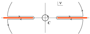
This contour can then be deformed and wrapped around the cuts along the real axis, as illustrated in the figure 7. Because the structure function is the discontinuity of across the cut, we can write
| (32) |
Therefore, we see that the OPE gives the -moments of the DIS structure functions.
In order to go further and calculate the perturbative Wilson coefficients , we must now identify the twist 2 operators that may contribute to DIS. In a theory of fermions and gauge bosons, we can construct two kinds of twist 2 operators :
| (33) |
where the brackets denote a symmetrization of the indices and a subtraction of the traced terms on those indices. To compute the Wilson coefficients, the simplest method is to exploit the fact that they are independent of the target. Therefore, we can take as the “target” an elementary object, like a quark or a gluon, for which everything can be computed in closed form (including the ). Consider first a quark state as the target, of a given flavor and spin . At lowest order, one has
| (34) |
Averaging over the spin, and comparing with , we get
| (35) |
On the other hand, we have already calculated directly the hadronic tensor for a single quark. By computing the moments of the corresponding , we get the for even :
| (36) |
From this, the bare Wilson coefficients for the operators involving quarks are
| (37) |
By repeating the same steps with a vector boson state, those involving only gluons are
| (38) |
if the vector bosons are assumed to be electrically neutral.
Going back to a nucleon target, we cannot compute the . However, we can hide momentarily our ignorance by defining functions and (respectively the quark and antiquark distributions) such that151515DIS with exchange of a photon cannot disentangle the quarks from the antiquarks. In order to do that, one could scatter a neutrino off the target, so that the interaction proceeds via a weak charged current.
| (39) |
(The sum is known as the singlet quark distribution of flavor .) Thus, the OPE formulas for and on a nucleon in terms of these quark distributions are
| (40) |
We see that these formulas have the required properties: (i) Bjorken scaling and (ii) the Callan-Gross relation.
Despite the fact that the OPE in a free theory of quarks and gluons leads to a result which is embarrassingly similar to the much simpler calculation we performed in the naive parton model, this exercise has taught us several important things :
-
•
We can derive an operator definition of the parton distributions (albeit it is not calculable perturbatively)
-
•
Bjorken scaling can be derived from first principles in a field theory of free quarks and gluons. This was a puzzle pre-QCD because clearly these partons are constituents of a strongly bound state.
-
•
The puzzle could be resolved if the field theory of strong interactions became a free theory in the limit , a property known as asymptotic freedom.
As shown by Gross, Politzer and Wilczek in 1973, non-Abelian gauge theories with a reasonable number of fermionic fields (e.g. QCD with 6 flavors of quarks) are asymptotically free[1] and were therefore a natural candidate for being the right theory of the strong interactions.
2.5 Scaling violations
Although it was interesting to see that a free quantum field theory reproduces the Bjorken scaling, this fact alone does not tell much about the detailed nature of the strong interactions at the level of quarks and gluons. Much more interesting are the violations of this scaling that arise from these interactions and it is the detailed comparison of these to experiments that played a crucial role in establishing QCD as the theory of the strong interactions.
The effect of interactions can be evaluated perturbatively in the framework of the OPE, thanks to renormalization group equations. In the previous discussion, we implicitly assumed that there is no scale dependence in the moments of the quark distribution functions. But this is not entirely true; when interactions are taken into account, they depend on a renormalization scale . The parton distributions become scale dependent as well. However, since are observable quantities that can be extracted from a cross-section, they cannot depend on any renormalization scale. Thus, there must also be a dependence in the Wilson coefficients, that exactly compensates the dependence originating from the . By dimensional analysis, the Wilson coefficients have an overall power of set by their dimension (see the discussion following eq. (29)), multiplied by a dimensionless function that can only depend on the ratio . By comparing the Callan-Symanzik equations[12] for with those for the expectation values , the renormalization group equation[12] obeyed by the Wilson coefficients is 161616We have used the fact that the electromagnetic currents are conserved and therefore have a vanishing anomalous dimension. Note also that we have exploited the fact that for twist 2 operators depends only on , so that we can replace by .
| (41) |
where is the beta function, and is the matrix of anomalous dimensions for the operators of spin (it is not diagonal because operators with identical quantum numbers can mix through renormalization).
In order to solve these equations, let us first introduce the running coupling such that
| (42) |
Note that this is equivalent to and ; in other words, is the value at the scale of the coupling whose value at the scale is . The usefulness of the running coupling stems from the fact that any function that depends on and only through the combination obeys the equation
| (43) |
It is convenient to express the Wilson coefficients at the scale from those at the scale as
| (44) |
In QCD, which is asymptotically free, we can approximate the anomalous dimensions and running coupling at one loop by
| (45) |
(The are obtained from a 1-loop perturbative calculation.) In this case, the scale dependence of the Wilson coefficients can be expressed in closed form as
| (46) |
From this formula, we can write the moments of the structure functions,
| (47) |
(and a similar formula for ). We see that we can preserve the relationship between and the quark distributions, eq. (40), provided that we let the quark distributions become scale dependent in such a way that their moments read
| (48) |
By also calculating the scale dependence of , one could verify that the Callan-Gross relation is preserved at the 1-loop order. It is crucial to note that, although we do not know how to compute the expectation values at the starting scale , QCD predicts how the quark distribution varies when one changes the scale . We also see that, in addition to a dependence on , the singlet quark distribution now depends on the expectation value of operators that involve only gluons (when the index in the previous formula).
The scale dependence of the parton distributions can also be reformulated in the more familiar form of the DGLAP equations. In order to do this, one should also introduce a gluon distribution , also defined by its moments,
| (49) |
Then one can check that the derivatives of the moments of the parton distributions with respect to the scale are given by
| (50) |
where we have used the shorthands . In order to turn this equation into an equation for the parton distributions themselves, one can use
| (51) |
that relates the product of the moments of two functions to the moment of a particular convolution of these functions. Using this result, and defining splitting function from their moments,
| (52) |
it is easy to derive the DGLAP equation[5],
| (53) |
that resums powers of . This equation for the parton distributions has a probabilistic interpretation : the splitting function can be seen as the probability that a parton splits into two partons separated by at least (so that a process with a transverse scale will see two partons), one of them being a parton that carries the fraction of the momentum of the original parton.
At 1-loop, the coefficients in the anomalous dimensions are
| (54) |
where is the number of flavors of quarks. On can note that, since is flavor independent, the non-singlet171717Here, the word “singlet” refers to the flavor of the quarks. linear combinations ( with ) are eigenvectors of the matrix of anomalous dimensions, with an eigenvalue . These linear combinations do not mix with the remaining two operators, and , through renormalization. By examining these anomalous dimensions for , we can see that the eigenvalue for the non-singlet quark operators is vanishing : . Going back to the eq. (50), this implies that
| (55) |
for any linear combination such that . This relation implies for instance that the number of quarks minus the number of quarks does not depend on the scale , which is due to the fact that the splittings produce quarks of all flavors in equal numbers (if one neglects the quark masses). An interesting relation can also be obtained for . For this moment, the matrix of anomalous dimensions in the singlet sector,
| (56) |
has a vanishing eigenvalue, which means that a linear combination of the flavor singlet operators is not renormalized : . This leads also to a sum rule
| (57) |
whose physical interpretation is the conservation of the total momentum of the proton – which therefore cannot depend on the resolution scale . (Collinear splittings, that are responsible for the dependence of the number of partons, do not alter their total momentum.)
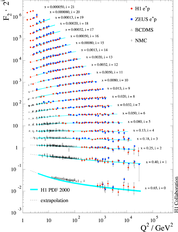
We have seen that QCD can be used to calculate the value of the Wilson coefficients as well as the scale dependence of the non-perturbative parton distributions. In practice, when one compares DIS data with theoretical predictions, one needs only to adjust the value of the parton distributions at a relatively low initial scale , and then one uses the DGLAP evolution equations in order to obtain their value at a higher . This program has now been implemented to three loops (NNLO), and has been very successful in explaining the inclusive DIS data. The agreement between QCD and the DIS measurements is illustrated in figure 8 (see for instance [13] for more details).
3 Lecture II : Parton evolution at small and gluon saturation
In the first lecture, we introduced the parton model and the evolution of parton distributions with the transverse resolution scale – and the corresponding resummation of the powers of . We now turn to the logarithms of . These logarithms are expected to be the dominant effect in processes where the collision energy is much larger than the typical transverse momentum scale involved in the process, and may lead to gluon saturation at very small .
3.1 Eikonal scattering
Before going to the main subject of this lecture, let us make a detour through an important result concerning the high energy limit of the scattering amplitude of some state off an external field. Our derivation here follows [14]. Consider the generic -matrix element
| (58) |
for the transition from a state to a state where
| (59) |
is the evolution operator from to . ( denotes an ordering in the light-cone time .) The interaction Lagrangian contains both the self-interactions of the fields and their interactions with the external field. Now apply a boost in the direction to all the particles contained in the states and . Formally, this can be done by multiplying the states by , where is the rapidity of the boost and the generator of longitudinal boosts. Our goal is to compute the limit of the transition amplitude,
| (60) |
The behavior of scattering amplitudes in this limit is easy to understand. The time spent by the incoming particles in the region where the external field is acting goes to zero as the inverse of the collision energy . If the coupling to the external field was purely scalar, this would imply that the scattering amplitude itself goes to zero as . However, in the case of a vector coupling, the longitudinal component of the current increases as , which compensates the decrease in the interaction time, thereby leading to a finite (non-zero and non infinite) high energy limit.
For this reason, let us assume that the coupling of the fields to the external potential is of the form where is a vector current built from the elementary fields of the theory under consideration. In order to simplify the discussion, we also assume that the external potential is non-zero only in a finite range in , (this is to avoid complications with long range interactions). The action of on states and operators is
| (61) |
namely, it multiplies the component of momenta by and their minus component by , while keeping the transverse components unchanged. The external potential is unaffected by , and the components of are changed as follows:
Because does not modify the ordering in , we can write
| (62) |
In addition, we can split the evolution operator into three factors
| (63) |
so that only the factor in the middle contains the external field. In order to deal with the first and last factor after the boost, it is sufficient to change variables , . This leads to
| (64) |
where is the same as , but with the self-interactions only. For the factor , the change of variables gives us
| (65) |
| (66) |
Only the minus component of the external vector potential matters, because this is the component that couples to the longitudinal current which is enhanced by the boost. Therefore, the high energy limit of the transition amplitude can be written as
| (67) |
This limit is known as the eikonal limit. It is important to keep in mind that this formula is the exact answer for the high-energy limit; no perturbative expansion has been made yet, and the formula still contains the self-interactions of the fields of the theory to all orders. A remarkable feature of eq. (67) is that it separates the self-interactions of the fields and their interactions with the external potential in three different factors, a property which is strongly suggestive of the factorization between the long and short distance physics in high energy hadronic interactions.
In order to use eq. (67) in practice, it is necessary to make an expansion in the self-interactions of the fields, by introducing complete sets of states between the three factors,
| (68) |
The factor is the Fock expansion of the initial state. It reflects the fact that the state prepared at may have fluctuated into another state before it interacts with the external potential. There is also a similar expansion for the final state. Assuming that we have performed the Fock expansion to the desired order181818The main difference compared to the usual perturbation theory is that the integrations over run only over half of the real axis, e.g. . In Fourier space, this implies that the minus component of the momentum is not conserved at the vertices, and that one gets energy denominators instead of delta functions., one needs to evaluate matrix elements such as
| (69) |
We have reinstated color indices in this formula, since we have applications to QCD in mind. In order to calculate this matrix element, the first step is to express the operator in terms of creation and annihilation operators of the particles that can couple to the external potential. For instance, the contribution that comes from the quarks and antiquarks is given by
| (70) |
(The quarks come with a positive sign and the antiquarks with a negative sign.) The contribution of the gluons would be similar, but the color matrix would be replaced by an element of the adjoint representation. From this formula, we see that in eq. (69), the states and must have the same particle content, because each annihilation operator in is immediately followed by a creation operator that creates a particle of the same nature. The component of the momenta of the particles in and must also be identical. The only difference between the states and is in the transverse momenta and in the color of their particles. In order to recover the eikonal limit in a more familiar form, one should go to impact parameter representation by performing a Fourier transformation of all the transverse momenta in the intermediate states and , by defining the light-cone wavefunction
| (71) |
Then, from the explicit form of , it is easy to check that the only effect of the external potential is to multiply the function by a phase factor for each particle in the intermediate state :
| (72) |
In the case of non-abelian interactions, these phase factors are known as Wilson lines. Wilson lines resum multiple scatterings off the external field, as one can see by expanding the exponential. Thus, the physical picture of high energy scattering off some external field is that the initial state evolves from to , multiply scatters during an infinitesimally short time off the external potential, and evolves again from to to form the final state, as illustrated in figure 9.
In terms of light-cone wavefunctions and of Wilson lines, the high energy limit of the transition amplitude reads
| (73) |
3.2 BFKL equation
Let us now derive the BFKL equation. Our derivation is inspired from [15, 16, 17, 18, 19]. Consider the forward scattering off an external field of a state whose simplest Fock component is a color singlet quark-antiquark pair. Thus, the transition amplitude can be written as
| (74) |
We will not need to specify more the light-cone wavefunction of the state under consideration. Note that the product of the two Wilson lines is traced, because the state is color singlet. A crucial property of this transition amplitude is that it is completely independent of the collision energy. However, as we shall see, a non trivial energy dependence arises in this amplitude because of large logarithms in loop corrections.
Consider now the 1-loop corrections to this amplitude depicted in figure 10.
These 1-loop corrections all involve one additional gluon attached to the quark or antiquark lines. In some of the corrections, that we shall call real corrections, the gluon is present in the state that goes through the external field. In the other corrections, the virtual corrections, the gluon is just a fluctuation in the wavefunction of the initial or final state. The calculation of these diagrams is straightforward in the impact parameter representation. One simply needs the formula for the vertex :
| (75) |
where is the polarization vector of the gluon and its transverse momentum, and its expression in impact parameter space,
| (76) |
Armed with these tools, it is easy to obtain expressions such as
| (77) | |||||
and
| (78) | |||||
We find that the sum of all the virtual corrections reads
| (79) |
where for SU(N). In this formula, is the longitudinal momentum of the gluon. As one can see, there is a logarithmic divergence in the integration over this variable. The lower bound should arguably be some non-perturbative hadronic scale , and the upper bound must be the longitudinal momentum of the quark or antiquark that emitted the photon. Hence we have a , which is a large factor in the limit of high-energy (strictly speaking, the high-energy limit is ill defined because of these corrections). The calculation of the real corrections is a bit more involved. For instance, one has
| (80) | |||||
where is a Wilson line in the adjoint representation that represents the eikonal phase factor associated to the gluon ( is the impact parameter of the gluon). In order to simplify the real terms, we need the following relation between fundamental and adjoint Wilson lines,
| (81) |
and the Fierz identity obeyed by fundamental SU(N) matrices :
| (82) |
Thanks to these identities, one can rewrite all the real corrections in terms of the quantity Collecting all the terms, and summing real and virtual contributions, we obtain the following expression for the 1-loop transition amplitude
| (83) |
where we denote . This correction to the transition amplitude is not small when , which means that -loop contributions should be considered in order to resum all the powers . Here, we are just going to admit that this -loop calculation amounts to exponentiating the 1-loop result. In other words, eq. (83) is sufficient in order to obtain the derivative ,
| (84) |
It is customary to rewrite this equation in terms of -matrix elements, . The BFKL equation[4] describes the regime where is small, so that we can neglect the terms that are quadratic in . It reads :
| (85) |
One can verify easily that is a fixed point of this equation (the right hand side vanishes if one sets ), but that this fixed point is unstable (if one sets , the right hand side is positive). Since there are no other fixed points, solutions of the BFKL have an unbounded growth in the high energy limit (). This behavior however is not physical, because the unitarity of scattering amplitude implies that should not become greater than unity.
3.3 Balitsky-Kovchegov equation
The solution to the above problem was in fact already contained in eq. (84). When written in terms of without assuming that is small,
| (86) |
it has a non-linear term that confines to the range . Indeed, the presence of this quadratic term makes a stable fixed point of the equation. Therefore, the generic behavior of solutions of eq. (86) is that starts at small values at small and asymptotically reaches the value in the high energy limit. Eq. (86) is known as the Balitsky-Kovchegov equation[17, 18].
The interaction of a color singlet dipole with an external color field is a possible description of DIS, in a frame in which the virtual photon splits into a quark-antiquark pair long before it collides with the proton (the external color field would represent the proton target). Although it is legitimate to treat the proton as a frozen configuration of color field due to the brevity of the interaction, we do not know what this field is. Moreover, since this field is created by the partons inside the proton, that have a complicated dynamics, this color field must be different for each collision, and should therefore be treated as random. Therefore, in order to turn our dipole scattering amplitude into an object that we could use to compute the DIS cross-section at high-energy, we must average over all the possible configurations of the external field. Let us denote by this average. The effect of this average on the energy dependence of the amplitude is simply taken into account by taking the average of eq. (86). However, one sees that the evolution equation for involves in its right hand side the average of a product of two ’s, . Therefore, we do not have a closed equation anymore. An evolution equation for could be obtained by the same procedure, which would depend on yet another new object, and so on. At the end of the day, one in fact obtains an infinite hierarchy of nested equations, known as Balitsky’s equations[18].
It is only if one assumes that the averages of products of amplitudes factorize into products of averages,
| (87) |
that this hierarchy can be truncated into a closed equation which is identical to eq. (86) – the BK equation – with replaced by . This approximation amounts to drop certain correlations among the target fields, and is believed to be a good approximation for a large nucleus in the limit of a large number of colors[17].
3.4 Gluon saturation and Color Glass Condensate
The problem encountered with the indefinite growth of the solutions of the BFKL can be understood in terms of the behavior of the gluon distribution at small momentum fraction . Indeed, in the regime where the dipole scattering amplitude is still small, it can be calculated perturbatively,
| (88) |
where . This formula is an example of the duality that exists in the description of scattering processes at high energy. In the derivation of the BFKL and BK equations, we have treated the proton target as given once for all, and the energy dependence has been obtained by applying a boost to the dipole projectile. But, thanks to the fact that transition amplitudes are Lorentz invariant quantities, they can also be evaluated in a frame where the dipole is fixed, and the boost is applied to the proton. In this frame, the energy dependence of the scattering amplitude comes from the dependence of the proton gluon distribution.
Thus, an exponential behavior of is equivalent to an increase of the gluon distribution as a power of :
| (89) |
(This growth of the gluon distribution is due to gluon splittings.) However, the gluon distribution cannot grow at this pace indefinitely. Indeed, at some point, the occupation number of the gluons will become large and the recombination of two gluons – not included in the BFKL equation – will be favored. This phenomenon is known as gluon saturation[20].
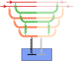
In the linear regime, described by the BFKL equation, each valence parton from the proton initiates its own gluon ladder (see figure 11) that evolves independently from the others. In the saturated regime, these gluon ladders can merge, thereby reducing the growth of the gluon distribution. The effect of these recombinations on the scattering amplitude is taken into account by the non-linear term of the BK equation.
A semi quantitative criterion for gluon saturation can be obtained[20] by comparing the surface density of gluons, , and the cross-section for gluon recombination, . Saturation occurs when , i.e. when
| (90) |
The quantity is known as the saturation momentum. Its dependence on the number of nucleons (in the case of a nuclear target) comes from the fact that scales like the volume, while is an area. Its dependence is a phenomenological parameterization inspired by from fits of HERA data.
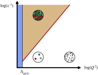
From eq. (90), one can divide the in two regions, as illustrated in figure 12. The saturated regime corresponds to the domain of low and low .
Although the BK equation describes the evolution of the dipole scattering amplitude into the saturation regime, there is an equivalent description of this evolution – the Color Glass Condensate – in which the central role is played by the target. The CGC description divides the degrees of freedom in the proton into fast partons (large ) and slow partons (small )[21]. The fast partons are affected by time dilation, and do not have any significant time evolution during the brief duration of the collision; therefore, they are treated as static objects that carry a color source. These color sources produce a current,
| (91) |
written here for a projectile moving in the direction. The function describes the distribution of color charge as a function of the impact parameter. The slow partons, on the other hand, have a non trivial dynamics during the collision, and must be treated as gauge fields. The only coupling between the fast and slow partons is a coupling between the color current of the fast partons and the gauge fields, which allows the fast partons to radiate slower partons by bremsstrahlung. Because the configuration of the fast partons prior to the collision is different in every collision, the function must be a stochastic quantity, for which one can only specify a distribution . Observables like cross-sections must be averaged over all the possible configurations of with this distribution. In fact, in the CGC description, this averaging procedure is equivalent to the target average of the scattering amplitude that was introduced in the discussion of the BK equation,
| (92) |
A crucial point is that the distribution depends on , the rapidity that separates what is considered fast and slow. Because such a separation is arbitrary, physical quantities cannot depend on it; one can derive from this requirement a renormalization group equation for – known as the JIMWLK equation[22] –, of the form :
| (93) |
The JIMWLK Hamiltonian contains first and second derivatives with respect to the source ,
| (94) |
where and are known functionals of . In fact, the JIMWLK equation is equivalent to the infinite hierarchy of Balitsky’s equations – of which the BK is an approximation that neglects some correlations. In the CGC description of scattering processes, the energy dependence of amplitudes arises from the dependence of the distribution . For instance, the dipole scattering amplitude would be written as
| (95) |
where the Wilson line is evaluated in the color field generated by the configuration of the color sources. This formula is very similar – at least in spirit – to the standard collinear factorization in DIS. The functional can be seen as an extension of the usual concept of parton distribution, that contains information about parton correlations beyond the mere number of partons, while the square bracket is the analogue of the “perturbative cross-section”. This formula is a Leading Logarithm (LL) factorization formula in the sense that it resums all the powers . Moreover, it also resums all the rescattering corrections, in , a feature which is not included in collinear factorization.
Eq. (93) predicts the energy dependence of the distribution of sources. However, it must be supplemented by an initial condition at some . As with the DGLAP equation, the initial condition is non-perturbative, and one must in general model it or guess it from experimental data. In the case of large nuclei, one often uses the McLerran-Venugopalan model, which assumes that is a Gaussian[21, 23, 24] :
| (96) |
The idea behind this model is that the color charge per unit area, , is the sum of the color charges of the partons that sit at approximately the same impact parameter. In a large nucleus, this will be the sum of a large number of random charges; for , this leads to a Gaussian distribution for plus a small (albeit physically very relevant) contribution from the cubic Casimir [24]. The fact that this Gaussian has only correlations local in impact parameter is a consequence of confinement : color charges separated by more than the nucleon size cannot be correlated. The MV model is generally used at a moderately small , of the order of . If the problem under consideration requires smaller values of , one should use the BK or JIMWLK equations, with the MV distribution as the initial condition.
3.5 Analogies with reaction-diffusion processes
There are interesting analogies between the evolution equations that govern the energy dependence of scattering amplitude in QCD and simple models of reaction-diffusion processes[25]. The simplest setting in which these correspondences can be seen is to consider the dipole scattering amplitude off a large nucleus, and to assume translation and rotation invariance in impact parameter space. It is useful to define its Fourier transform as
| (97) |
(Note the factor included in this definition.) It turns out that for this object , the BK equation has a very simple non-linear term,
| (98) |
In this equation, and with . The function has poles at and , and a minimum at . By expanding it up to quadratic order around its minimum, and by defining new variables,
| (99) |
the BK equation simplifies into
| (100) |
known as the Fisher-Kolmogorov-Petrov-Piscounov (FKPP) equation. This equation has been extensively studied in the literature, because it is the simplest realization of the so-called reaction-diffusion processes. It describes the evolution of a number of objects that live in one spatial dimension. The diffusion term describes the fact that these entities can hop from one location to neighboring locations. The positive linear term means that an object can split into two, and the negative quadratic term that two objects can merge into a single one. One can easily check that this equation has two fixed points, which is unstable and which is stable.
An important property of this equation is that it admits asymptotic travelling waves as solutions. Let us assume that the initial condition goes to at and to at , with an exponential tail . If the slope of the exponential obeys , the solution at late time depends only on a single variable,
| (101) |
When , the logarithm can be neglected in front of the term linear in time, and one has a travelling wave moving at a constant velocity without deformation (see figure 13).
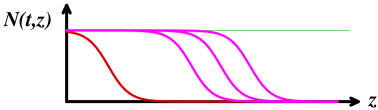
Moreover, this velocity is independent of the details of the initial condition for a large class of initial conditions.
Going back to the dipole scattering amplitude, this result implies the following scaling behavior at large :
| (102) |
with a saturation scale of the form
| (103) |
(The exponential comes from the constant in the velocity of the travelling wave, and the power law correction comes from the subleading logarithm.)
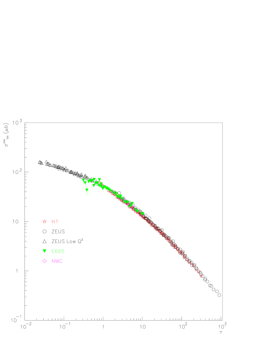
This scaling property has an interesting phenomenological consequence for the inclusive DIS cross-section, that one can express in terms of the forward dipole scattering amplitude thanks to the optical theorem :
| (104) |
In this formula, is the light-cone wave function for a photon of virtuality that splits into a quark-antiquark dipole of size , the quark carrying the fraction of the longitudinal momentum of the photon. This wavefunction can be calculated in QED, and its only property that we need here is that it depends only on the combination where is the quark mass. If one neglects the quark mass, then eq. (102) implies a simple scaling for the cross-section itself :
| (105) |
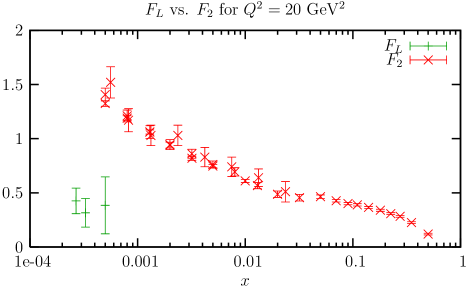
Such a geometrical scaling[26] has been found in the DIS experimental results191919In addition to explaining geometrical scaling, saturation inspired fits of DIS data are quite successful at small . See [27]., as shown in figure 14. A comment is in order here; as the approach based on collinear factorization and the DGLAP equation succeeds at reproducing much of the inclusive DIS data, it certainly also reproduces this scaling that is present in the data. However, this approach does not provide an explanation for the scaling. It arises via some fine tuning of the initial condition for the DGLAP evolution. In contrast, in the Color Glass Condensate description of DIS, this scaling is almost automatic.
4 Lecture III : Nucleus-nucleus collisions in the CGC framework
4.1 Introduction
Up to now, we only considered DIS, in which a possibly saturated proton or nucleus is probed by an elementary object202020Proton-nucleus collisions also belong to this category. Examples of processes have been studied in[28]. – a virtual photon that has fluctuated into a quark-antiquark dipole. In such a situation, the scattering amplitude can be written in closed form as a product of Wilson lines, and its energy dependence can be obtained either from Balitsky’s equations or from the JIMWLK evolution of the distribution of sources that produce the color field of the proton. There are however interesting problems that involve two densely occupied projectiles.
The archetype of such a situation is a high-energy nucleus-nucleus collision. In these collisions, one of the main challenges is to calculate the multiplicity of the particles (gluons at leading order) that are produced at the impact of the two nuclei. In the Color Glass Condensate framework, one has to couple the gauge fields to a current that receives contributions from the color sources of the two projectiles,
| (106) |
The fact that there are two strong sources leads to complications that are two-fold :
-
•
there is no explicit formula that gives the multiplicity (or any other observable) in terms of Wilson lines in the collision of two saturated projectiles,
-
•
if one is interested by the particle spectrum at some rapidity , one must evolve the two projectiles from their respective beam rapidity to . The question of the factorization of the large logarithms of is now much more complicated than in DIS.
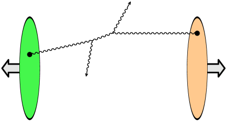
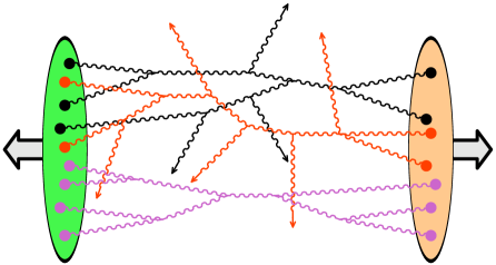
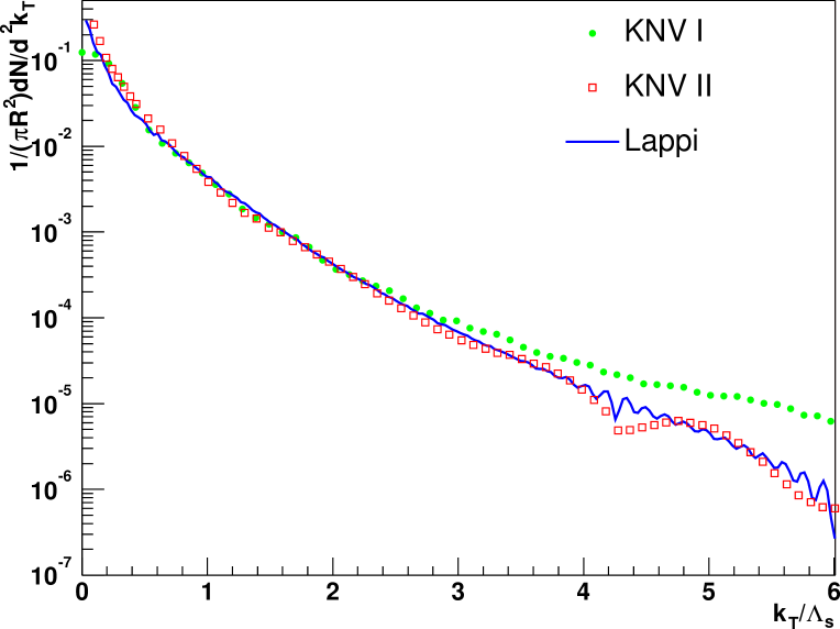
The kind of complications one is facing in this problem is illustrated in figure 15. In the saturated regime, reactions initiated by more than one parton (color source in the CGC description) in each projectile become important. Moreover, there can be a superposition of many independent scatterings, that will appear as disconnected graphs.
4.2 Power counting and bookkeeping
In the saturated regime, the color density (represented by dots in figure 15) is non-perturbatively large . This is due to the fact that the occupation number, proportional to , is of order in this regime. Thus for a connected graph, the order in is given by
| (107) |
where is the number of produced gluons and the number of loops. One can see that this formula is independent of the number of sources attached to the graph. Indeed, since each source brings a factor and is attached at a vertex that brings a factor , each source counts as a factor . If the diagram under consideration is made of several disconnected subgraphs, one should apply eq. (107) to each of them separately.
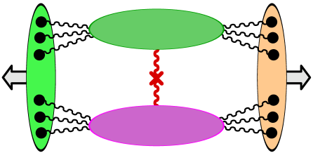
Among all the diagrams that appear in the calculation of particle production, a special role is played by the so-called vacuum diagrams – diagrams that have external gluons. They only connect sources of the two projectiles, and are thus contributions to the vacuum-to-vacuum amplitude , hence their name. The order of connected vacuum diagrams is . An extremely useful property is that the sum of all the vacuum diagrams (connected or not) is the exponential of those that are connected (that we denote where is the external current due to the color sources of the two projectiles)
| (108) |
The reason why vacuum diagrams are important in our problem is that it is possible to write all the time ordered products of fields – that enter in the reduction formulas for gluon production amplitudes – as derivatives of
| (109) |
Thanks to this property, one can write a very compact formula for the probability of producing exactly gluons in the collision[29, 30, 31],
| (110) |
where the operator is defined by212121We are a bit careless here with the Lorentz indices, polarization vectors, etc, because our main goal is to highlight the general techniques for keeping track of the diagrams that contribute to particle production in the saturated regime.
An important point to keep in mind about eq. (110) is that the external currents must be kept distinct in the amplitude and complex conjugate amplitude until all the derivatives contained in have been taken. Only then one is allowed to set and to the physical value of the external current. The propagator , that has only on-shell momentum modes, is the usual cut propagator that appears in Cutkosky’s cutting rules[12, 32]. The operator acts on cut vacuum graphs by removing two sources (one on each side of the cut, i.e. a and a ), and by connecting the points where they were attached by the cut propagator . In fact, since is obtained by acting times with the operator , it is the sum of all the cut vacuum diagrams in which exactly propagators are cut. Eq. (110) also makes obvious the fact that the probabilities do not have a meaningful perturbative expansion in the saturated regime, because the sum of the connected vacuum diagrams starts at the order .
By summing eq. (110) from to while keeping and distinct, one obtains the sum of all the cut vacuum diagrams with the current in the amplitude and in the complex conjugate amplitude to be
| (111) |
When we set , this sum becomes , and therefore it should be equal to 1 because of unitarity. Eq. (110) is very useful, because it allows to replace infinite sets of Feynman diagrams by simple algebraic equations. Similarly, the fact that eq. (111) is 1 when corresponds to a cancellation of an infinite set of graphs222222This cancellation is closely related to the Abramovsky-Gribov-Kancheli cancellation[33]., that would be very difficult to see at the level of diagrams.
4.3 Inclusive gluon spectrum
Eq. (110) leads to compact formulas for moments of the distribution of produced particles. The first moment – the average multiplicity – reads[29]
| (112) |
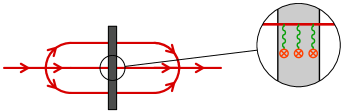
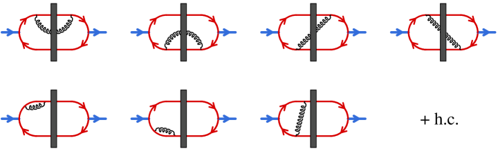
With the help of eq. (111), this formula tells us that is given by the action of the operator on the sum of all the cut vacuum diagrams. In plain english, this translates into : take a cut vacuum diagram (connected or not), remove a source on each side of the cut, and put a cut propagator where the sources were attached. Depending on whether the cut vacuum diagram one starts from is connected or not, one gets two different topologies, displayed in figure 16.
Each of the blobs in these diagrams can be any connected graph, and must be cut in all the possible ways232323Note that by not performing the integration contained in the explicit cut propagator, one obtains the inclusive gluon spectrum instead of the integrated multiplicity.. Thus, only connected graphs contribute to the multiplicity.
An important point is that, even though the perturbative expansion for the is not well defined, the multiplicity (and more generally any moment of the distribution ) can be organized in a sensible perturbative series242424The fact that this is possible for but not for the ’s themselves is due to the fact that the only graphs that contribute to are connected. This is a consequence of the AGK cancellation.. The Leading Order is obtained by keeping only the leading order vacuum graphs, i.e. those that have no loops :
| (113) |
Thus starts at the order . In eq. (113), for each tree diagram, one must sum over all the possible ways of cutting its lines. The simplest way of doing this is to use Cutkosky’s rules :
-
•
assign or labels to each vertex and source of the graph, in all the possible ways (there are terms for a graphs with vertices and sources). A vertex has a coupling and a vertex has a coupling ,
-
•
the propagators depend on which type of labels they connect. In momentum space, they read :
(114)
A quick analysis shows that, when one sets , summing over the labels at each vertex produces combinations of propagators,
| (115) |
where is the retarded propagator252525In momentum space, . Therefore, in coordinate space, it is proportional to , hence its name.. Thus, for a given tree graph, doing the sum over the cuts simply amounts to replacing all its propagators by retarded propagators. The last step is to perform the sum over all the trees. It is a well known result that the sum of all the tree diagrams that end at a point is a solution of the classical equations of motion of the field theory under consideration. In our case, this sum is a color field that obeys the Yang-Mills equations
| (116) |
where is the color current associated to the sources that represent the incoming projectiles (see eq. (106)). The boundary conditions obeyed by depend on the nature of the propagators that entered in the sum of tree diagrams. When these propagators are all retarded, one gets a retarded solution of the Yang-Mills equations, that vanishes in the remote past, . The precise formula for the gluon spectrum in terms of this solution of the Yang-Mills equations reads
| (117) |
Note that, although the integrations over and look 4-dimensional, they can be rewritten as 3-dimensional integrals evaluated at , thanks to the identity
| (118) |
Solving the Yang-Mills equations is an easy problem in the case of a single source , but turns out to be very challenging when there are two sources moving in opposite directions. The Schwinger gauge, defined by the constraint , is quite useful because it alleviates the need to ensure that the current is covariantly conserved262626In general gauges, one has to enforce the condition (this is a consequence of Jacobi’s identity for commutators). Because this relation involves a covariant derivative rather than an ordinary derivative, the radiated field leads to modifications of the current itself.. In this gauge, where and conversely, which makes this condition trivial. Moreover, in this gauge, one can find the value of the gauge field on a time-like surface just above the light-cone (at a proper time ) simply by matching the singularities across the light-cone. These initial conditions[34] can be written as272727An interesting feature of the gauge fields at early times after the collision – a phase recently named “glasma” – is that the chromo-electric and magnetic fields are purely longitudinal, while they were transverse to the beam axis just before the collision[35].
| (119) |
where . In this formula, and are the gauge fields created by each nucleus111Because retarded solutions are causal, the field below the light-cone cannot depend simultaneously on and . below the light-cone :
Therefore, the problem of solving the Yang-Mills equations from to is reduced to solving them in the forward light-cone from a known initial condition222Note that at , the YM equations are the vacuum ones, since all the sources are located on the light-cone..
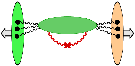
Since our problem is invariant under boosts in the direction, one can completely eliminate the space-time rapidity from the equations of motion (and the initial conditions in eq. (119) are also -independent). Thus, in the forward light-cone, one has to solve numerically[36] equations of motion in time and two spatial dimensions, and then to evaluate eq. (117). The result of this computation is displayed in figure 17.
In this computation, the MV model was used as the distribution of the sources and . Therefore, the dependence of the spectrum on the momentum rapidity of the produced gluon cannot be obtained in this calculation, and only the dependence is shown. The main effect of gluon recombinations on this spectrum is that it reduces the yield at low transverse momentum, . Indeed, in a fixed order calculation in perturbative QCD, the spectrum would behave as . In the CGC picture, the singularity of the spectrum at low is only logarithmic333If the final Fourier decomposition is performed at a finite time , the spectrum is completely regular when ., and is therefore integrable.
4.4 Inclusive quark spectrum
A similar study has also been performed for the initial production of quarks in nucleus-nucleus collisions[37]. The starting point is to construct for quarks an operator that plays the same role as the operator defined in eq. (4.2) :
| (121) |
where is the free cut fermionic propagator and where is a Grassmanian current that couples to the spinors. In terms of this operator, the probability of producing quarks is given by :
| (122) |
The first thing to note is that now the connected vacuum diagrams, whose sum is , depend on both the source and on the source . However, the latter is set to zero at the end of the calculation, because in the CGC one assumes that the color sources in the wavefunction of the projectiles couple only to the gluons. Therefore, the source serves only as an intermediate bookkeeping device. Another important point in this formula is the presence of the factor . This factor means that we are calculating an inclusive probability, for producing exactly quarks possibly accompanied by an arbitrary number of gluons444Without this factor, we would be calculating the probability of producing quarks and gluons. Note that in principle, we should also modify our definition of the probability of producing gluons by a factor . However, the quarks are a subleading correction compared to the gluons, and this change would not affect the gluon spectrum at leading order.. In practice, this fact means that one must sum over all the possible ways of cutting the gluons lines in the diagrams that contribute to quark production. From eq. (122), one obtains the following formula for the average number of produced quarks
| (123) |
In this formula, the underlined factors represent the sum of all (connected or not) the cut vacuum diagrams made of quarks and gluons, with sources on one side of the cut, and sources on the other side. Acting on a term of this sum with removes a source and a source , and connect the points where these sources were attached by a cut fermion propagator. Diagrammatically, this corresponds to the two topologies displayed in figure 18.
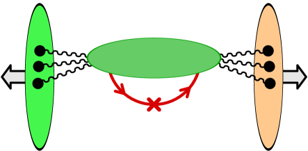
Note however that the topology that appears on the left of figure 18 cannot exist because it has a quark line which is not closed onto itself (this is forbidden since we set the fermionic sources to zero at the end of this calculation). Thus, we only have the second family of diagrams, that have at least one loop. This means that the average number of quarks is of order , compared to the number of gluons which is of order .
The leading contribution to the quark multiplicity is obtained by including only tree diagrams in the blob. Thus, we have to sum all the graphs that have one quark loop (with an explicit cut on it) and any number of gluonic trees attached to it, and all the cuts thereof. The sum of all the gluonic trees and their cuts has already been encountered in the computation of the gluon multiplicity : it is equal to the retarded solution of the Yang-Mills equations that vanish in the remote past. Therefore, the quark spectrum is given by
| (124) |
where is the cut quark propagator on which the retarded classical field has been resummed. This resummed propagator can be obtained as the solution of the equation
| (125) |
where (we need only the combination in eq. (124), but the four terms get mixed when one resums the background field). It is possible to decouple these equations by performing a “rotation” on the indices[38],
| (126) |
| (127) |
After this rotation, the propagator matrix becomes triangular,
| (128) |
with and the resummed retarded and advanced propagators and where . The main simplification comes from the fact that the product of the free matrix propagator and of is the sum of a diagonal and a nilpotent matrix, which makes the calculation of its -th power very easy555Indeed, with very formal notations, the resummed matrix propagator is . In particular, one finds that the equations that lead to the retarded (and also the advanced) propagator do not mix with anything else,
| (129) |
and that the resummed can be expressed in terms of as666The symbol denotes the convolution of 2-point functions: .
| (130) |
At this point, one must invert the rotation done in eq. (126) in order to obtain which is needed in the formula for the quark spectrum. This gives the quark spectrum in terms of retarded quantities,
where is the “scattering part” of the retarded propagator, related to by
| (131) |
The last step is to write this object in terms of retarded solutions of the Dirac equation in the background field . It is easy to check that
| (132) |
In this formula, and are the usual free spinors. Note that the initial condition for the Dirac equation is a negative energy spinor, and that the projection performed at the final time is with a positive energy spinor. In the vacuum, there would be no overlap between these spinors. However, since in our problem the spinor travels on top of a time-dependent background field, it acquires positive energy modes which make non zero.
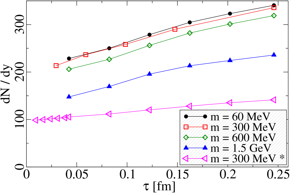
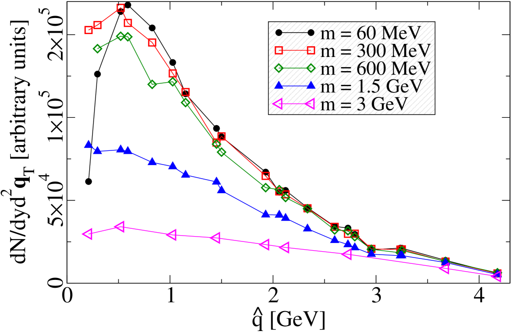
This formulation of quark production in the CGC framework has been implemented numerically, also with the MV model for the average over the configurations of the color sources . Similarly to what happened with the gluons, one can obtain analytically the value of the spinors just above the light-cone. Hence, the numerical resolution of the Dirac equation is only needed in the forward light-cone. However, there is a major difference compared to the gluons at LO : even though the background color field does not depend on rapidity, this is not true of the solutions of Dirac equation777This has nothing to do with the fact that we are considering fermions, but rather with the quark spectrum being a NLO quantity – that involves a loop in the background of the classical field.. Indeed, the momentum in the initial condition renders the spinors dependent on the space-time rapidity (the boost invariance of the background field implies that the spinors depend only on the difference where is the rapidity of the momentum ). This difference makes the computation of the quark spectrum much more computationally intensive relative to that of the gluon spectrum, because one has to keep the three dimensions of space. Some of the results obtained are displayed in figure 19. On the left plot is shown the time dependence of the quark yield, for different quark masses (i.e. the yield obtained by performing the projection in eq. (132) at a finite time instead of taking the limit ). One can see that a good fraction of the quarks are produced at , when the two nuclei pass through each other888In the analogous QED problem of production in the high-energy collision of two electrical charges, all the electrons are produced at and their number does not change at . This is because in QED, the electro-magnetic potential in the forward light-cone is a pure gauge, that could be made to vanish by a gauge transformation. and that the number slightly increases in time afterwards due to the color field present in the forward light-cone. The right panel of figure 19 shows the dependence of the spectrum for various quark masses. As expected, the spectrum is harder for larger quark masses. Note that the tail of the curves is probably affected by important lattice artifacts due to a too coarse lattice.
4.5 Loop corrections to the gluon spectrum
Thus far, we limited ourselves to the leading order contribution for both the gluons and the quarks. However, we a priori know from figures 16 and 18 what diagrams contribute to the gluon and quark multiplicities to all orders. There is therefore a well defined and systematic procedure to compute corrections to the previous results. Loop corrections to gluon production are very relevant for the following reasons:
-
•
They contain terms that are divergent due to unbounded integrals over longitudinal momenta, very similar to the divergences encountered in the derivation of the BK equation. One should verify whether these divergences can be absorbed in the distributions and of the color sources of each projectile. This factorization is crucial for the internal consistency of the CGC framework.
-
•
It has been noted recently that the boost invariant solution of the Yang-Mills equations is unstable999This instability is very similar to the Weibel instability that occurs in anisotropic plasmas[39],[40].; rapidity dependent perturbations to this solution grow exponentially in time. Loop corrections generate this kind of rapidity dependent perturbations. Tracking all these terms and resumming them is very important in order to get meaningful answers from the CGC regarding the momentum distribution of the produced gluons, and may be relevant in the problem of thermalization in heavy ion collisions.
Note that these two items address very different stages of the collision process. The first relates to the incoming wavefunctions (and as such should be independent of the subsequent collision), while the second issue is about what happens in the final state after the collision. Therefore, we should aim at writing the 1-loop corrections in a way that separates the initial and final state as clearly as possible.
Let us start by listing the relevant diagrams : the 1-loop corrections to the average multiplicity are shown in the diagrams of figure 20.
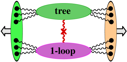
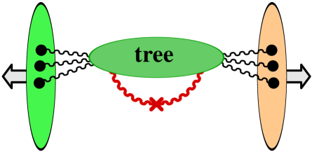
The topology on the left is very similar to the one already encountered at tree level, except that one of the blobs has now a loop correction in it. The topology on the right is new; but it is in fact similar to what we had to evaluate in the case of the quark spectrum, except that the fermionic cut propagator must be replaced by the cut propagator of a gluon. The NLO contribution to the gluon spectrum can be written as
| (133) | |||||
The two terms of the first line are the contribution of the diagram on the left of figure 20 (the loop can be in either of the two blobs), and the term on the second line comes from the diagram on the right. The field that appears on the first line is the 1-loop correction to ; and it obeys the linearized equation of motion for small fluctuations.
Let us now illustrate how one can separate the initial state from the final state in the term that contains . First, by analogy with the case of the quarks, we can write
| (134) |
where is a small fluctuation of the gauge field on top of , with initial condition when . The equation of motion of this fluctuation is obtained by writing the Yang-Mills equations for and by linearizing it in . A central formula in order to separate the initial and final states is the following101010To avoid encumbering the equations with indices of various kinds, we are suppressing all the indices in this and the following formula.
| (135) |
where denotes a point located on the light-cone () ( represents any set of three coordinates that map the light-cone.) In this formula, the classical field is considered as a functional of its initial condition on the light-cone. The notation is a shorthand for
| (136) |
(In this formula, the 4-vector is a vector normal111111 if is a small displacement on the light-cone at the point under consideration. to the light-cone.) The proof of eq. (135) is straightforward121212Write the Green’s formula that expresses in terms of the initial , insert it in eq. (135), and check that this leads to the Green’s formula that relates to its initial condition ., but its diagrammatic interpretation is more interesting.
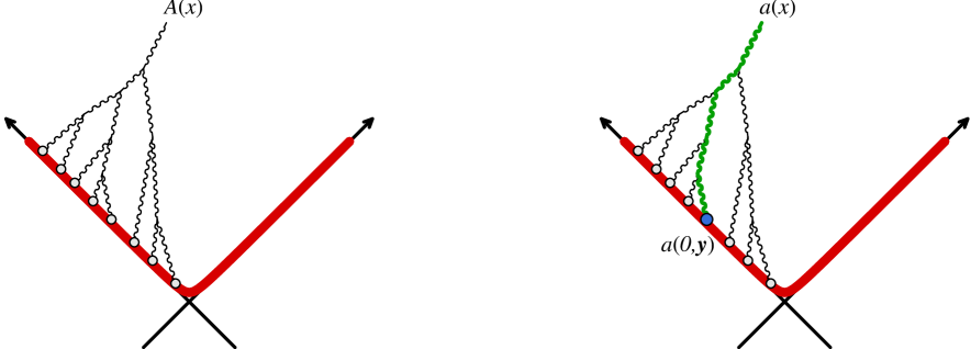
Note first that , seen as a functional of its initial condition on the light-cone, can also be represented by tree diagrams, as illustrated in the left panel of figure 21. (This can be seen from the Green’s formula for .) The action of the operator defined in eq. (136) on the classical field is to replace one of the open dots in figure 21 by the fluctuation , represented by a filled dot in the right panel of figure 21. The diagram one gets after this is nothing but a contribution to the propagation of a small fluctuation over the classical field. Plugging eq. (135) in eq. (134), this quantity becomes
The brackets are crucial in this formula, in order to limit the scope of the derivatives contained in the operators and . Note that, if it were not for these brackets, the first line and the two ’s of the second line would be nothing but the LO gluon spectrum. It turns out that, after one adds the contribution of the first line in eq. (133), the NLO correction to the spectrum can be written as
| (138) |
where the LO spectrum is considered as a functional of the initial classical field on the light-cone. In this equation, is the value of on the light-cone, and the 2-point is defined as
| (139) |
Note that and are in principle calculable analytically.
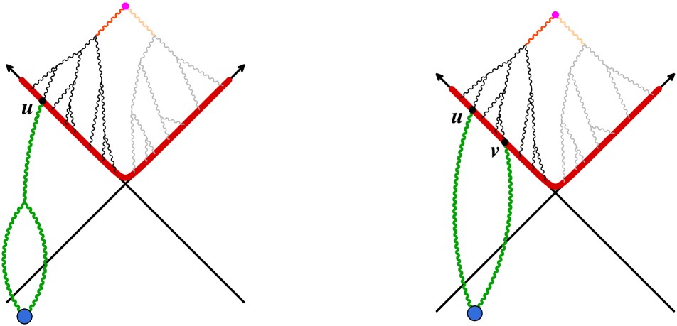
Eq. (138) realizes the separation we were seeking of the initial and final states. Indeed, the operator in the square bracket depends only on what happens below the light-cone, i.e. before the collision. On the contrary, the LO spectrum seen as a functional of the initial classical field depends only on the final state dynamics. The other benefit of this formula is that is expresses the NLO correction as a perturbation of the LO one; this property – that seems generalizable to other inclusive observables – suggests the universality of the initial state divergences and their factorizability.
From eq. (138), it is easy to see what are the potential sources of divergences. A first issue is that the coefficients and are infinite. For for instance, the integration over the longitudinal component of the momentum in eq. (139) diverges. A similar divergence occurs in the loop contained in . The fact that these divergences arise in the first factor of eq. (138) indicates that they are related to the evolution of the initial projectiles prior to the collision. These divergences can be momentarily regularized by introducing cutoffs in rapidity around the rapidity at which the spectrum is calculated. Thus, and become finite but depend on these unphysical cutoffs. To be consistent, the distribution of the sources and should be evolved from the beam rapidities to and respectively. Thus, the complete formula for the LO+NLO spectrum, including the average over the sources, should be
| (140) |
where the subscript and superscript indicate that the momentum integrals contained in the bracket have cutoffs in rapidity. Recall that the LO spectrum in the right hand side is a function of on the light-cone, which is itself a function of . The factorizability of these divergences in the initial state is equivalent to the independence of the previous formula with respect to the unphysical and . Let us for instance change into . According to the JIMWLK equation, the distribution of is modified by
| (141) |
At the same time, the operator in the right hand side varies by
| (142) |
At this point, one can verify that the terms linear131313Note that, since we have only considered 1-loop corrections, this independence can only be satisfied for small variations of the cutoff, at linear order in these variations. in cancel provided that
| (143) |
Similar considerations on the dependence give another condition :
| (144) |
Therefore, in order to check whether one can factorize these divergences in the JIMWLK evolution of the incoming sources, one must calculate the coefficients and – or at least their divergent part – and remap the operator into the JIMWLK Hamiltonian. Although this program has not been fully implemented yet, one can already note that the structure of makes this outcome very plausible.
Eq. (138) also allows us to discuss the issue of the instability of the boost invariant classical solution. These instabilities manifest themselves in the fact that the action of on diverges when the time goes to infinity. Indeed,
| (145) |
is a measure of how is sensitive to its initial condition.
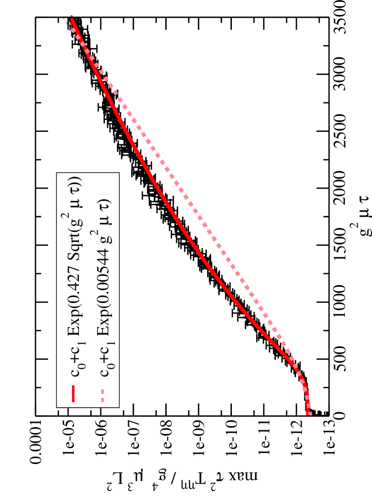
Therefore, if the solution is unstable, small perturbations of its initial condition lead to exponentially growing changes in the solution. From the numerical study of these instabilities (see figure 23), one gets[39]
| (146) |
where is of the order of the saturation momentum. This means that, although the 1-loop corrections are suppressed by a factor compared to the LO, some of these corrections are enhanced by factors that grow exponentially in time after the collision. At first sight, one may expect a complete breakdown of the CGC description at
| (147) |
i.e. the time at which the 1-loop corrections become as large as the LO contribution. The only way out of this conclusion is to resum all these enhanced corrections in the hope that the resummed series is better behaved when . Let us assume for the time being that we have performed this resummation, and that the sum of these enhanced terms generalize eq. (138) to read
| (148) |
where is a certain functional of the operator . In the right hand side, we have emphasized the fact that the LO spectrum is a functional of the initial classical field on the light-cone. This formula can be written in a more intuitive way by performing a Fourier transform of ,
| (149) |
In this formula, the functional integration is in fact an integration over two fields : the fluctuation itself and its derivative normal to the light-cone . Thanks to the fact that is the generator of translations of the initial conditions on the light-cone, the exponential in the previous formula is the translation operator itself. Therefore, when this exponential acts on a functional of the initial classical field , it gives the same functional evaluated with a shifted initial condition . Therefore, we can write
| (150) |
We see that the effect of the resummation is simply to add fluctuations to the initial conditions of the classical field, with a distribution that depends on the details of the resummation141414In a recent work by one of the authors, using a completely different approach, the spectrum of initial fluctuations was found to be Gaussian[41].. It is easy to understand why these fluctuations are crucial in the presence of instabilities : despite the fact that they are suppressed by an extra power of , the instabilities make them grow and eventually become as large as the LO. One can also see that the resummation has the effect of lifting the time limitation of eq. (147). Indeed, after the resummation, the fluctuation has entered in the initial condition for the full Yang-Mills equation, whose non-linearities prevent the solution from blowing up. A very important question is whether these instabilities fasten the local thermalization of the system formed in heavy ion collisions.
4.6 Summary and outlook
If the initial state factorization works as expected, and after the resummation of the leading contributions of the instability, the formula for the gluon spectrum should read
| (151) | |||||
This formula resums the most singular terms at each order in . Because of their relation to the physics of the initial and final state respectively, the distributions generalize parton distributions, while plays a role similar to that of a fragmentation function151515Naturally, this function has nothing to do with a gluon fragmenting into a hadron. Instead, it is related to how classical fields become gluons..
Note that, even after the resummations performed in the initial and final states of eq. (151), this formula still suffers from the usual problem of collinear gluon splitting in the final state. This is not a serious concern in heavy ion collisions though, because collinear singularities occur only when one takes the limit, and we do expect to have to switch to another description (like hydrodynamics) long before this becomes a problem. In fact, the initial condition for hydrodynamics should be specified in terms of the energy-momentum tensor, which is infrared and collinear safe because it measures only the flow of energy and momentum.
A more important problem, that has still not received a satisfactory answer, is to understand how the initial particle spectrum – or the local energy momentum-tensor – become isotropic. This requires formulating a kinetic theory of the glasma which describes how particles emerge from the decaying classical field and their subsequent interactions both with the classical field and with other particles. Recently, such a kinetic equation has been derived for a scalar field theory coupled to strong sources [42]. Extending this work to QCD and exploring its consequences- in particular, the approach of the particle+field system towards equilibration remains a challenging problem.
Acknowledgements
FG would like to thank the organizers – and in particular D. P. Menezes – of the Xth Hadron Physics Workshop held in Florianopolis, Brazil, for their invitation to give these lectures and for the nice and stimulating atmosphere of the meeting, as well as the hospitality of M.B. Gay-Ducati at the UFRGS, and of E.S. Fraga and T. Kodama at the UFRJ. FG also acknowledges the financial support of CAPES-COFECUB under project #443-04. TL and RV are supported by DOE Contract No. DE-AC02-98CH10886.
References
- [1] D.J. Gross, F. Wilczek, Phys. Rev. Lett. 30, 1343 (1973), Phys. Rev. D 8, 3633 (1973), Phys. Rev. D 9, 980 (1974); H.D. Politzer, Phys. Rev. Lett. 30, 1346 (1973), Phys. Rept. 14, 129 (1974).
- [2] S. Catani, M. Ciafaloni, F. Hautmann, Nucl. Phys. B 366, 135 (1991); J.C. Collins, R.K. Ellis, Nucl. Phys. B 360, 3 (1991).
- [3] J.C. Collins, D.E. Soper, G. Sterman, Nucl. Phys. B 250, 199 (1985), ibid. 261, 104 (1985), ibid. 263, 37 (1986).
- [4] E.A. Kuraev, L.N. Lipatov, V.S. Fadin, Sov. Phys. JETP 45, 199 (1977); I. Balitsky, L.N. Lipatov, Sov. J. Nucl. Phys. 28, 822 (1978).
- [5] V.N. Gribov, L.N. Lipatov, Sov. J. Nucl. Phys. 15, 438 (1972), ibid. 15, 675 (1972); Yu. Dokshitzer, Sov. Phys. JETP 46, 641 (1977); G. Altarelli, G. Parisi, Nucl. Phys. B 126, 298 (1977).
- [6] S.D. Drell, J.D. Walecka, Annals Phys. 28, 18 (1964).
- [7] E.D. Bloom, et al., Phys. Rev. Lett. 23, 930 (1969); M. Breidenbach, et al., Phys. Rev. Lett. 23, 935 (1969).
- [8] J.D. Bjorken, Phys. Rev. 148, 1467 (1966), SLAC-PUB-0571, (1969).
- [9] C.G. Callan, D.J. Gross, Phys. Rev. Lett. 22, 156 (1969).
- [10] R.P. Feynman, Photon-Hadron Interactions, Frontiers in Physics, W.A. Benjamin, (1972); J.D. Bjorken, Lecture Notes in Physics, 56, Springer, Berlin (1976).
- [11] K.G. Wilson, Phys. Rev. 179, 1499 (1969).
- [12] M.E. Peskin, D.V. Schroeder, An introduction to quantum field theory, Addison-Wesley, New-York (1995).
- [13] J. Gayler, [H1 and ZEUS collaborations] hep-ex/0603037.
- [14] J.D. Bjorken, J.B. Kogut, D.E. Soper, Phys. Rev. D 3, 1382 (1971).
- [15] H. Weigert, Nucl. Phys. A 703, 823 (2002).
- [16] Yu.V. Kovchegov, Phys. Rev. D 60, 034008 (1999).
- [17] Yu.V. Kovchegov, Phys. Rev. D 61, 074018 (2000).
- [18] I. Balitsky, Nucl. Phys. B 463, 99 (1996).
- [19] A.H. Mueller, Phys. Lett. B 523, 243 (2001).
- [20] L.V. Gribov, E.M. Levin, M.G. Ryskin, Phys. Rept. 100, 1 (1983); A.H. Mueller, J-W. Qiu, Nucl. Phys. B 268, 427 (1986); J.P. Blaizot, A.H. Mueller, Nucl. Phys. B 289, 847 (1987).
- [21] L.D. McLerran, R. Venugopalan, Phys. Rev. D 49, 2233 (1994), ibid. 49, 3352 (1994), ibid. 50, 2225 (1994).
- [22] J. Jalilian-Marian, A. Kovner, L.D. McLerran, H. Weigert, Phys. Rev. D 55, 5414 (1997); J. Jalilian-Marian, A. Kovner, A. Leonidov, H. Weigert, Nucl. Phys. B 504, 415 (1997), Phys. Rev. D 59, 014014 (1999), ibid. 034007 (1999), ibid. erratum, 099903 (1999); E. Iancu, A. Leonidov, L.D. McLerran, Nucl. Phys. A 692, 583 (2001), Phys. Lett. B 510, 133 (2001); E. Ferreiro, E. Iancu, A. Leonidov, L.D. McLerran, Nucl. Phys. A 703, 489 (2002).
- [23] Yu.V. Kovchegov, Phys. Rev. D 54, 5463 (1996).
- [24] S. Jeon, R. Venugopalan, Phys. Rev. D 70, 105012 (2004), ibid. 71, 125003 (2005).
- [25] S. Munier, R. Peschanski, Phys. Rev. Lett. 91, 232001 (2003), Phys. Rev. D 69, 034008 (2004), ibid. 70, 077503 (2004).
- [26] A.M. Stasto, K. Golec-Biernat, J. Kwiecinski, Phys. Rev. Lett. 86, 596 (2001); E. Iancu, K. Itakura, L.D. McLerran, Nucl. Phys. A 708, 327 (2002); C. Marquet, L. Schoeffel, Phys. Lett. B 639, 471 (2006); F. Gelis, R. Peschanski, L. Schoeffel, G. Soyez, Phys. Lett. B.647, 376 (2007).
- [27] K. Golec-Biernat, M. Wüsthoff, Phys. Rev. D 59, 014017 (1999), ibid. 60, 114023 (1999); J. Bartels, K. Golec-Biernat, H. Kowalski, Phys. Rev. D 66, 014001 (2002); E. Iancu, K. Itakura, S. Munier, Phys. Lett. B 590, 199 (2004).
- [28] Yu.V. Kovchegov, A.H. Mueller, Nucl. Phys. B 529, 451 (1998); A. Kovner, U. Wiedemann, Phys. Rev. D 64, 114002 (2001); Yu.V. Kovchegov, K. Tuchin, Phys. Rev. D 65, 074026 (2002); A. Dumitru, L.D. McLerran, Nucl. Phys. A 700, 492 (2002); A. Dumitru, J. Jalilian-Marian, Phys. Rev. Lett. 89, 022301 (2002), Phys. Lett. B 547, 15 (2002); F. Gelis, J. Jalilian-Marian, Phys. Rev. D 67, 074019 (2003); J.P. Blaizot, F. Gelis, R. Venugopalan, Nucl. Phys. A 743, 13 (2004), ibid. 57 (2004); F. Gelis, Y. Methar-Tani, Phys. Rev. D 73, 034019 (2006); N.N. Nikolaev, W. Schafer, Phys. Rev. D 71, 014023 (2005); J. Jalilian-Marian, Y. Kovchegov, Prog. Part. Nucl. Phys. 56, 104 (2006); F. Gelis, J. Jalilian-Marian, Phys. Rev. D 66, 014021 (2002), ibid. 094014, (2002); J. Jalilian-Marian, Nucl. Phys. A 753, 307 (2005); F. Gelis, J. Jalilian-Marian, hep-ph/0609066.
- [29] F. Gelis, R. Venugopalan, Nucl. Phys. A 776, 135 (2006).
- [30] F. Gelis, R. Venugopalan, Nucl. Phys. A 779, 177 (2006).
- [31] F. Gelis, R. Venugopalan, Acta Phys. Polon. B 37, 3253 (2006), hep-ph/0611157.
- [32] R.E. Cutkosky, J. Math. Phys. 1, 429 (1960).
- [33] V.A. Abramovsky, V.N. Gribov, O.V. Kancheli, Sov. J. Nucl. Phys. 18, 308 (1974).
- [34] A. Kovner, L.D. McLerran, H. Weigert, Phys. Rev. D 52, 6231 (1995).
- [35] T. Lappi, L.D. McLerran, Nucl. Phys. A 772, 200 (2006).
- [36] A. Krasnitz, R. Venugopalan, Nucl. Phys. B 557, 237 (1999), Phys. Rev. Lett. 84, 4309 (2000), ibid. 86, 1717 (2001); A. Krasnitz, Y. Nara, R. Venugopalan, Nucl. Phys. A 727, 427 (2003), Phys. Rev. Lett. 87, 192302 (2001); T. Lappi, Phys. Rev. C 67, 054903 (2003).
- [37] F. Gelis, K. Kajantie, T. Lappi, Phys. Rev. C. 71, 024904 (2005), Phys. Rev. Lett. 96, 032304 (2006).
- [38] A.J. Baltz, F. Gelis, L.D. McLerran, A. Peshier, Nucl. Phys. A 695, 395 (2001).
- [39] P. Romatschke, R. Venugopalan, Phys. Rev. Lett. 96, 062302 (2006), Eur. Phys. J. A 29, 71 (2006), Phys. Rev. D D 74, 045011 (2006).
- [40] S. Mrowczynski, Phys. Lett. B 214, 587 (1988), ibid. 314, 118 (1993), ibid. 363, 26 (1997); S. Mrowczynski, M.H. Thoma, Phys. Rev.D 62, 036011 (2000); A.K. Rebhan, P. Romatschke, M. Strickland, Phys. Rev. Lett. 94, 102303 (2005), JHEP 0509, 041 (2005); P. Arnold, J. Lenaghan, G.D. Moore, JHEP 0308, 002 (2003); P. Arnold, J. Lenaghan, G.D. Moore, L.G. Yaffe, Phys. Rev. Lett. 94, 072302 (2005).
- [41] K. Fukushima, F. Gelis, L. McLerran, Nucl. Phys. A 786, 107 (2007).
- [42] F. Gelis, S. Jeon, R. Venugopalan, arXiv:0706.3775 [hep-ph].