Sparse and stable Markowitz portfolios

Abstract

We consider the problem of portfolio selection within the classical Markowitz mean-variance framework, reformulated as a constrained least-squares regression problem. We propose to add to the objective function a penalty proportional to the sum of the absolute values of the portfolio weights. This penalty regularizes (stabilizes) the optimization problem, encourages sparse portfolios (i.e. portfolios with only few active positions), and allows to account for transaction costs. Our approach recovers as special cases the no-short-positions portfolios, but does allow for short positions in limited number. We implement this methodology on two benchmark data sets constructed by Fama and French. Using only a modest amount of training data, we construct portfolios whose out-of-sample performance, as measured by Sharpe ratio, is consistently and significantly better than that of the naïve evenly-weighted portfolio which constitutes, as shown in recent literature, a very tough benchmark.

Keywords:

Portfolio Choice, Sparsity, Penalized Regression

1 Introduction

In 1951, Harry Markowitz ushered in the modern era of portfolio theory by applying simple mathematical ideas to the problem of formulating optimal investment portfolios (Markowitz, 1952). Single minded pursuit of high returns constitutes a poor strategy, Markowitz argued. Instead, he suggested, rational investors must balance a desire for high returns with a desire for low risk, as measured by variability of returns.

It is not trivial, however, to translate Markowitz’s conceptual framework into a satisfactory portfolio selection algorithm in a real-world context. Indeed, in a recent survey, DeMiguel, Garlappi, and Uppal (2007) examined several portfolio construction algorithms inspired by the Markowitz framework. The authors found that, given a reasonable amount of training data, none of the surveyed algorithms is able to significantly or consistently outperform the naïve strategy in which each available asset is given an equal weight in the portfolio. This disappointing algorithm performance is likely due, at least in part, to the structure of the Markowitz optimization framework as originally proposed. Specifically, the optimization at the core of the Markowitz scheme is, as originally formulated, empirically unstable: small changes in assumed asset returns, volatilities or correlations can have large effects on the output of the optimization procedure. In this sense, the classic Markowitz portfolio optimization can be viewed as an ill-posed (or ill-conditioned) inverse problem. Such problems are frequently encountered in many other fields, where a variety of regularization procedures have been proposed to tame the troublesome instabilities (Bertero and Boccacci, 1998).

In this paper, we discuss a regularization of Markowitz’s portfolio construction. We shall restrict ourselves to the traditional Markowitz mean-variance approach; moreover, we focus on one particular regularization method, and highlight some very special properties of the regularized portfolios obtained through its use.

Our proposal consists of adding an $\ell_{1}$ penalty to the Markowitz objective function. We allow ourselves to adjust the importance of this penalty with a “tunable” coefficient. For large values of this coefficient, optimization of the penalized objective function turns out to be equivalent to solving the original (unpenalized) problem under an additional positivity condition on the weights. As the tunable coefficient is decreased, the optimal solutions are given more and more latitude to include short positions. The optimal solutions for our penalized objective function can thus be seen as natural generalizations of the “no-short-positions” portfolios considered by Jagannathan and Ma (2003). In addition to stabilizing the optimization problem (Daubechies, Defrise, and De Mol, 2004) and generalizing no-short-positions-constrained optimization, the $\ell_{1}$ penalty facilitates treatment of transaction costs. For large investors, whose principal cost is a fixed bid-ask spread, transaction costs are effectively proportional to the gross market value of the selected portfolio, and thus to our $\ell_{1}$ penalty term. For small investors, volume independent “overhead” costs cannot be ignored, and thus transaction costs are best modeled via a combination of an $\ell_{1}$ penalty term and the number of assets transacted; minimizing such a combination is tantamount to searching for sparse solutions (sparse portfolios or sparse changes to portfolios), a goal that we shall see is also achieved by our use of an $\ell_{1}$ penalty term.

We implement the methodology and compute efficient investment portfolios using as our assets two sets of portfolios constructed by Fama and French: the 48 industry portfolios and the 100 portfolios formed on size and book-to-market. Using data from 1973 to 2006, we construct an ensemble of portfolios for various values of our tunable coefficient and track their out-of-sample performances. We find a consistent and significant increase in Sharpe ratio compared to the naïve equal-weighting strategy. When using the 48 industry portfolios as our assets, we find that the best portfolios we construct have no short positions. When our assets are the 100 portfolios formed on size and book-to-market, we find that the best portfolios constructed by our methodology do include short positions.

We are not alone in proposing the use of regularization in the context of Markowitz-inspired portfolio construction; DeMiguel, Garlappi, Nogales, and Uppal (2007) discuss several different regularization techniques for the portfolio construction problem, including the imposition of constraints on appropriate norms of the portfolio weight vector. Our work differs from DeMiguel, Garlappi, Nogales, and Uppal (2007) in that our goal is not only regularization: we are interested in particular in the stable construction of sparse portfolios, which is achieved by $\ell_{1}$ penalization, as demonstrated by our analysis and examples.

The organization of our paper is as follows. In the next Section, we formulate the problem of portfolio selection and we describe our methodology based on $\ell_{1}$-penalized least-squares regression. In Section 3, we describe key mathematical properties of the portfolios we construct and devise an efficient algorithm for computing them. In Section 4, we present empirical results consisting of an out-of-sample performance evaluation of our sparse portfolios. In Section 5, we discuss possible extensions of our methodology to other portfolio construction problems which can be naturally translated into optimizations involving $\ell_{1}$ penalties. Finally, Section 6 summarizes our findings.

2 Sparse portfolio construction

We consider $N$ securities and denote their returns at time $t$ by $r_{i,t}$, $i=1,\dots,N$. We write $\mathbf{r}_{t}=(r_{1,t},\ldots,r_{N,t})^{\top}$ for the $N\times 1$ vector of returns at time $t$. We assume that the returns are stationary and write $\mathbf{E}[\mathbf{r}_{t}]=\boldsymbol{\mu}$ for the vector of expected returns of the different assets, and $\mathbf{E}[(\mathbf{r}_{t}-\boldsymbol{\mu})(\mathbf{r}_{t}-\boldsymbol{\mu})^{\top}]=\boldsymbol{C}$ for the covariance matrix of returns.

A portfolio is defined to be a list of weights $w_{i}$ for assets $i=1,\ldots,N$ that represent the amount of capital to be invested in each asset. We assume that one unit of capital is available and require that capital to be fully invested. Thus we must respect the constraint that $\sum_{i=1}^{N}w_{i}=1$. We collect the weights in an $N\times 1$ vector $\mathbf{w}=(w_{1},\ldots,w_{N})^{\top}$. The normalization constraint on the weights can thus be rewritten as $\mathbf{w}^{\top}\mathbf{1}_{N}=1$, where $\mathbf{1}_{N}$ denotes the $N\times 1$ vector in which every entry is equal to 1. For a given portfolio $\mathbf{w}$, the expected return and variance are equal to $\mathbf{w}^{\top}\boldsymbol{\mu}$ and $\mathbf{w}^{\top}\boldsymbol{C}\mathbf{w}$, respectively.

In the traditional Markowitz portfolio optimization, the objective is to find a portfolio which has minimal variance for a given expected return $\rho=\mathbf{w}^{\top}\boldsymbol{\mu}$. More precisely, one seeks $\widetilde{\mathbf{w}}$ such that:

$$\widetilde{\mathbf{w}} = \arg\min_{\mathbf{w}}\mathbf{w}^{\top}\boldsymbol{C}\mathbf{w}$$

s. t. $$\mathbf{w}^{\top}\boldsymbol{\mu}=\rho$$

$$\mathbf{w}^{\top}\mathbf{1}_{N}=1.$$

Since $\boldsymbol{C}=\mathbf{E}[\mathbf{r}_{t}\mathbf{r}^{\top}_{t}]\,-\,\boldsymbol{\mu}\boldsymbol{\mu}^{\top}$, the minimization problem is equivalent to

$$\widetilde{\mathbf{w}} = \arg\min_{\mathbf{w}}\mathbf{E}\left[|\rho-\mathbf{w}^{\top}\mathbf{r}_{t}|^{2}\right]$$

s. t. $$\mathbf{w}^{\top}\boldsymbol{\mu}=\rho$$

$$\mathbf{w}^{\top}\mathbf{1}_{N}=1.$$

For the empirical implementation, we replace expectations with sample averages. We set $\widehat{\boldsymbol{\mu}}=\frac{1}{T}\sum_{t=1}^{T}\mathbf{r}_{t}$ and define $\boldsymbol{R}$ to be the $T\times N$ matrix of which row $t$ is given by $\mathbf{r}_{t}^{\top}$, that is, $\boldsymbol{R}_{t,i}=\left(\mathbf{r}_{t}\right)_{i}=r_{i,t}$. Given this notation, we thus seek to solve the following optimization problem

$$\widehat{\mathbf{w}} = \arg\min_{\mathbf{w}}\frac{1}{T}\|\rho\mathbf{1}_{T}-\boldsymbol{R}\mathbf{w}\|^{2}_{2}$$

s. t. $$\mathbf{w}^{\top}\widehat{\boldsymbol{\mu}}=\rho$$

$$\mathbf{w}^{\top}\mathbf{1}_{N}=1,$$

where, for a vector $\mathbf{a}$ in $\mathbb{R}^{T}$, we denote by $\|\mathbf{a}\|^{2}_{2}$ the sum $\sum_{t=1}^{T}\mathbf{a}_{t}^{2}$.

This problem requires the solution of a constrained multivariate regression involving many potentially collinear variables. While this problem is analytically simple, it can be quite challenging in practice, depending on the nature of the matrix $\boldsymbol{R}$. Specifically, the condition number — defined to be the ratio of the largest to smallest singular values of a matrix — of $\boldsymbol{R}$ can effectively summarize the difficulty we will face when trying to perform this optimization in a stable way. When the condition number of $\boldsymbol{R}$ is small, the problem is numerically stable and easy to solve. However, when the condition number is large, a non-regularized numerical procedure will amplify the effects of noise anisotropically, leading to an unstable and unreliable estimate of the vector $\mathbf{w}$. As asset returns tend to be highly correlated, the smallest singular value of $\boldsymbol{R}$ can be quite small, leading to a very large condition number and thus very unstable optimizations in a financial context. It is this sort of instability that likely plagues many of the algorithms reviewed by DeMiguel, Garlappi, and Uppal (2007) and renders them unable to outperform the naïve portfolio.

To obtain meaningful, stable results for such ill-conditioned problems, one typically adopts a regularization procedure. One fairly standard approach is to augment the objective function of interest with a penalty term, which can take many forms and ideally should have a meaningful interpretation in terms of the specific problem at hand. We propose here to add a so-called $\ell_{1}$ penalty to the original Markowitz objective function (2). We thus seek to find a vector of portfolio weights $\mathbf{w}$ that minimizes

$$\mathbf{w}^{[\tau]} = \arg\min_{\mathbf{w}}\left[||\rho\mathbf{1}_{T}-\boldsymbol{R}\mathbf{w}||^{2}_{2}+\tau||\mathbf{w}||_{1}\right]$$ (2)

s. t. $$\mathbf{w}^{\top}\widehat{\boldsymbol{\mu}}=\rho$$ (4)

$$\mathbf{w}^{\top}\mathbf{1}_{N}=1.$$

Here the $\ell_{1}$ norm of a vector $\mathbf{w}$ in $\mathbb{R}^{N}$ is defined by $\|\mathbf{w}\|_{1}:=\sum_{i=1}^{N}|w_{i}|~{}$, and $\tau$ is a parameter that allows us to adjust the relative importance of the $\ell_{1}$ penalization in our optimization. Note that we absorbed the factor $1/T$ from (2) in the parameter $\tau$. The particular problem of minimizing an (unconstrained) objective function of the type (2) was named lasso regression by Tibshirani (1996).

Adding an $\ell_{1}$ penalty to the objective function (2) has several useful consequences:

• It promotes sparsity. That penalizing or minimizing $\ell_{1}$ norms can have a sparsifying effect has long been observed in statistics (see e.g. Chen, Donoho, and Saunders (2001) and the references therein). Minimization of $\ell_{1}$ penalized objective functions is now a widely used technique when sparse solutions are desirable. Sparsity should also play a key role in the task of formulating investment portfolios. Indeed, investors frequently want to be able to limit the number of positions they must create, monitor and liquidate. By considering suitably large values of $\tau$ in (2), one can achieve just such an effect within our framework. Figure 1 illustrates geometrically how the addition of an $\ell_{1}$ term to the unconstrained volatility minimization encourages sparse solutions.

  

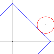
  (a) Very small $\ell_{1}$ penalty: tangency on edge.

  

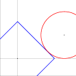
  (b) Small $\ell_{1}$ penalty: tangency on edge, nearing vertex.

  

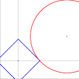
  (c) Moderately sized $\ell_{1}$ penalty: tangency reaches vertex.

  

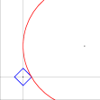
  (d) Large $\ell_{1}$ penalty: tangency remains at vertex, moves toward origin along axis.

  Figure 1: $\ell_{1}$ penalties promote sparsity: a geometric illustration in $2$ dimensions. In $N$ dimensions, the level sets of the $\ell_{1}$ norm are so-called cross polytopes , while the level sets of the volatility term (2) are typically ellipsoids. In 2 dimensions, we illustrate these as diamonds and circles respectively. The minimizer of (2) must be located at a point where the level sets of the $\ell_{1}$ term and the volatility term are tangent. There is a continuous family of such points, and the solution to a particular minimization will be determined by the relative sizes of the terms in the objective function (2). When the $\ell_{1}$ norm is given a small weight in the objective function, optimal solutions lie on level sets of large $\ell_{1}$ norm. These large $\ell_{1}$ level sets intersect the volatility level sets at generic points where many, if not all, of the entries in $\mathbf{w}$ differ from zero. However, as the weight on the $\ell_{1}$ term is increased, the tangency moves onto smaller level sets of the $\ell_{1}$ norm. Since the $\ell_{1}$ ball is “pointy,” the tangencies move toward the corners of the $\ell_{1}$ level sets where more and more entries in $\mathbf{w}$ are equal to $0$. Moreover, as Figure 2 shows, any $\ell_{p}$ penalty with $0\leqslant p\leqslant 1$ will lead to “pointy” level sets that give rise to a similar sparsification effect.

• It regulates the amount of shorting in the portfolio designed by the optimization process. Because of the constraint (4), an equivalent form of the objective function in (2) is

  $$\|\rho\mathbf{1}_{T}-\boldsymbol{R}\mathbf{w}\|^{2}_{2}+2\tau\!\!\!\sum_{i\mbox{ with }w_{i}<0}|w_{i}|\,+\,\tau,$$ (5)

  in which the last term is of course irrelevant for the optimization process. Under the constraint (4), the $\ell_{1}$ penalty is thus equivalent to a penalty on short positions.

  The no-short-positions optimal portfolio, obtained by minimizing (2) under the three constraints given by not only (4) and (4) but also the additional restriction $w_{i}\geqslant 0$ for $i=1,\ldots,N$, is in fact the optimal portfolio for (5) in the limit of extremely large values of $\tau$. As the high $\tau$ limit of our framework, it is completely natural that the positive solution should be quite sparse; this sparsity of optimal no-short-positions portfolios can indeed also be observed in practice. (See Section 4.) We note that the literature has focused on the stability of positive solutions, but seems to have overlooked the sparsity of such solutions. This may be due, possibly, to the use of iterative numerical optimization algorithms and a stopping criterion that halted the optimization before most of the components had converged to their zero limit. By decreasing $\tau$ in the $\ell_{1}$-penalized objective function to be optimized, one relaxes the constraint without removing it completely; it then no longer imposes positivity absolutely, but still penalizes overly large negative weights.

• It stabilizes the problem. By imposing a penalty on the size of the coefficients of $\mathbf{w}$ in an appropriate way, we reduce the sensitivity of the optimization to the possible collinearities between the assets. In Daubechies, Defrise, and De Mol (2004), it is proved (for the unconstrained case) that any $\ell_{p}$ penalty on $\mathbf{w}$, with $1\leqslant p\leqslant 2$, suffices to stabilize the minimization of (2) by regularizing the inverse problem. The stability induced by the $\ell_{1}$ penalization is extremely important; indeed, it is such stability property that makes practical, empirical work possible with only limited training data. For example, De Mol, Giannone, and Reichlin (2006) show that this regularization method can be used to produce accurate macroeconomic forecasts using many predictors. Figure 2 shows the geometric impact of an $\ell_{p}$ penalty for the unconstrained problem for various values of $p$. It also illustrates why only $\ell_{p}$ penalties with $0\leqslant p\leqslant 1$ are able to promote sparsity.

  

  

  

  

  Figure 2: A geometric look at regularization penalties. The panels above depict sets of fixed $\ell_{p}$ norm for various values of $p$ (from left to right, $p=1/2,1,2,3$), in 3 dimensions. For any fixed $p$, adding an $\ell_{p}$ penalty to a given minimization encourages solutions to stay within regions around the origin defined by scaled versions of the $\ell_{p}$ ball. For $p\geqslant 1$ the amended minimization problem remains convex, and thus algorithmically more tractable; on the other hand $\ell_{p}$ penalties with $0\leqslant p\leqslant 1$ encourage sparsity (see Figure 1). In our optimization, we focus on the case $p=1$, which has both desirable features.

• It makes it possible to account for transaction costs in a natural way. In addition to the choice of the securities they trade, real-world investors must also concern themselves with the transaction costs they will incur when acquiring and liquidating the positions they select. Transaction costs in a liquid market can be modeled by a two-component structure: one that is a fixed “overhead”, independent of the size of the transaction, and a second one, given by multiplying the transacted amount with the market-maker’s bid-ask spread applicable to the size of the transaction.

  For large investors, the overhead portion can be neglected; in that context, the total transaction cost paid is just $\sum_{i=1}^{N}s_{i}\,|w_{i}|$, the sum of the products of the absolute trading volumes $|w_{i}|$ and bid-ask spreads $s_{i}$ for the securities $i=1,\ldots,N$. We assume that the bid-ask spread is the same for all assets and constant for a wide range of transaction sizes. In that case, the transaction cost is then effectively captured by an $\ell_{1}$ penalty.

  For small investors, the overhead portion of the transaction costs is non negligible. In the case of a very small investor, this portion may even be the only one worth considering; if the transaction costs are asset-independent, then the total cost is simply proportional to the number $K$ of assets selected (i.e. corresponding to non-zero weights), a number sometimes referred to as $\|\mathbf{w}\|_{0}$, the $\ell_{0}$ norm of the weight vector. Like an $\ell_{1}$ sum, this $\ell_{0}$ sum can be incorporated into the objective function to be minimized; however, $\ell_{0}$-penalized optimization is computationally intractable when more than a handful of variables are involved because its complexity is essentially combinatorial in nature, and grows super-exponentially with the number of variables. For this reason, one often replaces the $\ell_{0}$ penalty, when it occurs, by its much more tractable (convex) $\ell_{1}$-penalty cousin, which has similar sparsity-promoting properties. In this sense, our $\ell_{1}$ penalization is thus “natural” even for small investors.

3 Optimization strategy

We first quickly review the unconstrained case, i.e. the minimization of the objective function (2), and then discuss how to deal with the constraints (4) and (4).

Various algorithms can be used to solve (2). For the values of the parameters encountered in the portfolio construction problem, a particularly convenient algorithm is given by the homotopy method (Osborne, Presnell, and Turlach, 2000a, b), also known as Least Angle Regression or LARS (Efron, Hastie, Johnstone, and Tibshirani, 2004). This algorithm seeks to solve (2) for a range of values of $\tau$, starting from a very large value, and gradually decreasing $\tau$ until the desired value is attained. As $\tau$ evolves, the optimal solution $\mathbf{w}^{[\tau]}$ moves through $\mathbb{R}^{N}$, on a piecewise affine path. As such, to find the whole locus of solutions for $\mathbf{w}^{[\tau]}$ we need only find the critical points where the slope changes. These slopes are thus the only quantities that need to be computed explicitly, besides the breakpoints of the piecewise linear (vector-valued) function. For every value of $\tau$, the entries $j$ for which $w_{j}\,\neq\,0$, are said to constitute the active set $\mathcal{A}_{\tau}$. Typically, the number of elements of $\mathcal{A}_{\tau}$ increases as $\tau$ decreases. However, this is not always the case: at some breakpoints entries may need to be removed from $\mathcal{A}_{\tau}$; see e.g. (Efron, Hastie, Johnstone, and Tibshirani, 2004).

When the desired minimizer contains only a small number $K$ of non-zero entries, this method is very fast. At each breakpoint, the procedure involves solving a linear system of $k$ equations with $k$ unknowns, $k$ being the number of active variables, which increases until $K$ is reached. This imposes a pragmatic feasibility upper bound on $K$.

The homotopy/LARS algorithm applies to the unconstrained $\ell_{1}$-penalized regression. The problem of interest to us, however, is the minimization of (2) under the constraints (4, 4), in which case the original algorithm does not apply. In the Appendix, we show how the homotopy/LARS algorithm can be adapted to deal with a general $\ell_{1}$-penalized minimization problem with linear constraints, allowing us to find:

$$\mathbf{w}^{[\tau]}=\arg\min_{\mathbf{w}\in H}\left[\|\mathbf{y}-\boldsymbol{R}\mathbf{w}\|^{2}_{2}+\tau\|\mathbf{w}\|_{1}\right]$$ (6)

where $H$ is a prescribed affine subspace, defined by the linear constraints. The adapted algorithm consists again of starting with large values of $\tau$, and shrinking $\tau$ gradually until the desired value is reached, monitoring the solution, which is still piecewise linear, and solving a linear system at every breakpoint in $\tau$. Because of the constraints, the initial solution (for large values of $\tau$) is now more complex (in the unconstrained case, it is simply equal to zero); in addition, extra variables (Lagrange multipliers) have to be introduced that are likewise piecewise linear in $\tau$, and the slopes of which have to be recomputed at every breakpoint.

In the particular case of the minimization (2) under the constraints (4), (4), an interesting interplay takes place between (4) and the $\ell_{1}$-penalty term. When the weights $w_{i}$ are all non-negative, the constraint (4) is equivalent to setting $\|\mathbf{w}\|_{1}\,=\,1$. Given that the $\ell_{1}-$penalty term takes on a fixed value in this case, minimizing the quadratic term only (as in (2)) is thus equivalent to minimizing the penalized objective function in (2), for non-negative weights $w_{i}$. This is consistent with the observation made by Jagannathan and Ma (2003) that a restriction to non-negative-weights-only can have a regularizing effect on Markowitz’s portfolio construction.

The following mathematical observations have interesting consequences. Suppose that the two weight vectors $\mathbf{w}^{[\tau_{1}]}$ and $\mathbf{w}^{[\tau_{2}]}$ are minimizers of (2), corresponding to the values $\tau_{1}$ and $\tau_{2}$ respectively, and both satisfy the two constraints (4), (4). By using the respective minimization properties of $\mathbf{w}^{[\tau_{1}]}$ and $\mathbf{w}^{[\tau_{2}]}$, we obtain

$$\|\rho\mathbf{1}_{T}-\boldsymbol{R}\mathbf{w}^{[\tau_{1}]}\|^{2}_{2}\,+\,\tau_{1}\|\mathbf{w}^{[\tau_{1}]}\|_{1} \leqslant \|\rho\mathbf{1}_{T}-\boldsymbol{R}\mathbf{w}^{[\tau_{2}]}\|^{2}_{2}\,+\,\tau_{1}\|\mathbf{w}^{[\tau_{2}]}\|_{1}$$

$$= \|\rho\mathbf{1}_{T}-\boldsymbol{R}\mathbf{w}^{[\tau_{2}]}\|^{2}_{2}\,+\,\tau_{2}\|\mathbf{w}^{[\tau_{2}]}\|_{1}$$

$$\qquad\qquad\,+\,(\,\tau_{1}-\tau_{2}\,)\,\|\mathbf{w}^{[\tau_{2}]}\|_{1}$$

$$\leqslant \|\rho\mathbf{1}_{T}-\boldsymbol{R}\mathbf{w}^{[\tau_{1}]}\|^{2}_{2}\,+\,\tau_{2}\|\mathbf{w}^{[\tau_{1}]}\|_{1}$$

$$\qquad\qquad\,+\,(\,\tau_{1}-\tau_{2}\,)\,\|\mathbf{w}^{[\tau_{2}]}\|_{1}$$

$$= \|\rho\mathbf{1}_{T}-\boldsymbol{R}\mathbf{w}^{[\tau_{1}]}\|^{2}_{2}\,+\,\tau_{1}\|\mathbf{w}^{[\tau_{1}]}\|_{1}$$

$$\,+\,(\,\tau_{1}-\tau_{2}\,)\,\left(\,\|\mathbf{w}^{[\tau_{2}]}\|_{1}-\|\mathbf{w}^{[\tau_{1}]}\|_{1}\,\right),$$

which implies that

$$(\,\tau_{1}\,-\,\tau_{2}\,)\,\left(\,\|\mathbf{w}^{[\tau_{2}]}\|_{1}\,-\,\|\mathbf{w}^{[\tau_{1}]}\|_{1}\,\right)\,\geqslant\,0.$$ (7)

If some of the $w_{i}^{[\tau_{2}]}$ are negative, but all the entries in $\mathbf{w}^{[\tau_{1}]}$ are positive or zero, then we have $\|\mathbf{w}^{[\tau_{2}]}\|_{1}\,>\,\left|\sum_{i=1}^{N}w_{i}^{[\tau_{2}]}\right|\,=\,1$; on the other hand, $\|\mathbf{w}^{[\tau_{1}]}\|_{1}\,=\,1$ (because the $w_{i}^{[\tau_{1}]}$ are all non-negative), implying $\|\mathbf{w}^{[\tau_{2}]}\|_{1}\,>\,\|\mathbf{w}^{[\tau_{1}]}\|_{1}$ . In view of (7), this means that $\tau_{1}\,\geqslant\,\tau_{2}$.

It follows that the optimal portfolio with non-negative entries obtained by our minimization procedure corresponds to the largest values of $\tau$, and thus typically to the sparsest solution (since the penalty term, promoting sparsity, is weighted more heavily). This particular portfolio is a minimizer of (2), under the constraints (4) and (4), for all $\tau$ larger than some critical value $\tau_{0}$. For smaller $\tau$ the optimal portfolio will contain at least one negative weight and will typically become less sparse. However, as in the unconstrained case, this need not happen in a monotone fashion.

Although other optimization methods could be used to compute the sparse portfolios we define, the motivation behind our choice of a constrained homotopy/LARS algorithm is the fact that we are only interested in computing portfolios involving only a small number of securities and that we use the parameter $\tau$ to tune this number. Whereas other algorithms would require separate computations to find solutions for each value of $\tau$, a particularly nice feature of our LARS-based algorithm is that, by exploiting the piecewise linear dependence of the solution on $\tau$, it obtains, in one run, the weight vectors for all values of $\tau$ (i.e. for all numbers of selected assets) in a prescribed range.

4 Empirical application

In this section we apply the methodology described above to construct optimal portfolios and evaluate their out-of-sample performance.

We present two examples, each of which uses a universe of investments compiled by Fama and French. In the first example, we use 48 industry sector portfolios (abbreviated to FF48 in the remainder of this paper). In the second example, we use 100 portfolios formed on size and book-to-market (FF100). In both FF48 and FF100, the portfolios are constructed at the end of each June.

4.1 Example 1: FF48

Using the notation of Section 2, $r_{i,t}$ is the annualized return in month $t$ of industry $i$, where $i=1,\ldots,48$. We evaluate our methodology by looking at the out-of-sample performances of our portfolios during the last 30 years in a simulated investment exercise.

Each year from 1976 to 2006, we construct a collection of optimal portfolios by solving an ensemble of minimizations of (2) with constraints (4) and (4). For each time period, we carry out our optimization for a sufficiently wide range of $\tau$ so as to produce an ensemble of portfolios containing different numbers of active positions; ideally we would like to construct portfolios with $K$ securities, for all values of $K$ between 2 and 48. As explained below, we do not always obtain all the low values of $K$; typically we find optimal portfolios only for $K$ exceeding a minimal value $K_{\mbox{\tiny{min}}}$, that varies from year to year. (See Figure 3). To estimate the necessary return and covariance parameters, we use data from the preceding 5 years (60 months). At the time of each portfolio construction, we set the target return, $\rho$, to be the average return achieved by the naïve, evenly-weighted portfolio over the previous 5 years.

For example, our first portfolio construction takes place at the end of June 1976. To determine $\boldsymbol{R}$ and $\widehat{\boldsymbol{\mu}}$, we use the historical returns from July 1971 until June 1976. We then solve the optimization problem using this matrix and vector, targeting an annualized return of $6.60\%$ ($\rho=0.066$), equal to the average historical return, from July 1971 until June 1976, obtained by a portfolio in which all industry sectors are given the equal weight 1/48. We compute the weights of optimal solutions $\mathbf{w}^{[\tau]}$ for $\tau$ ranging from large to small values. We select these portfolios according to some criterion we would like to meet. We could, e.g. target a fixed total number of active positions, or limit the number of short positions; see below for examples. Once a portfolio is thus fixed, it is kept from July 1976 until June 1977, and its returns are recorded. At the end of June 1977, we repeat the same process, using training data from July 1972 to June 1977 to compute the composition of a new collection of portfolios. These portfolios are observed from July 1977 until June 1978 and their returns are recorded. The same exercise is repeated every year with the last ensemble of portfolios constructed at the end of June 2005.

Once constructed, the portfolios are thus held through June of the next year and their monthly out-of-sample returns are observed. These monthly returns, for all the observation years together, constitute a time series; for a given period (whether it is the full 1976$\rightarrow$2006 period, or sub-periods), all the monthly returns corresponding to this period are used to compute the average monthly return $m$, its standard deviation $\sigma$, and their ratio $m/\sigma$, which is then the Sharpe ratio measuring the trade-off, corresponding to the period, between returns and volatility of the constructed portfolios.

We emphasize that the sole purpose of carrying out the portfolio construction multiple times, in successive years, is to collect data from which to evaluate the effectiveness of the portfolio construction strategy. These constructions from scratch in consecutive years are not meant to model the behavior of a single investor; they model, rather, the results obtained by different investors who would follow the same strategy to build their portfolio, starting in different years. A single investor might construct a starting portfolio according to the strategy described here, but might then, in subsequent years, adopt a sparse portfolio adjustment strategy such as described in Section 5.

We compare the performance of our strategy to that of a benchmark strategy comprising an equal investment in each available security. This $1/N$ strategy is a tough benchmark since it has been shown to outperform a host of optimal portfolio strategies constructed with existing optimization procedures (DeMiguel, Garlappi, and Uppal, 2007). To evaluate the $1/N$ strategy portfolios for the FF48 assets, we likewise observe the monthly returns for a certain period (a 5-year break-out period or the full 30-year period), and use them to compute the average mean return $m$, the standard deviation $\sigma$, and the Sharpe ratio $m/\sigma$.

We carried out the full procedure following several possible guidelines. The first such guideline is to pick the optimal portfolio $\mathbf{w}^{\mbox{\tiny{pos.}}}$ that has only non negative weights $w_{i}$, i.e. the optimal portfolio without short positions. As shown in Section 3, this portfolio corresponds to the largest values of the penalization constant $\tau$; it typically is also the optimal portfolio with the fewest assets. Figure 3 reports the number of active assets of this optimal no-short-positions portfolio from year to year. This number varies from a minimum of 4 to a maximum of 11, with an average of around 6; note that this is quite sparse in a 48 asset universe. Table 1 reports statistics to evaluate the performances of the optimal no-short-positions portfolio. We give the statistics for the whole sample period as well as for consecutive sub-periods extending over 5 years each, comparing these to the portfolio that gives equal weight to the 48 assets. The table shows that the optimal no-short-positions portfolio significantly outperforms the benchmark both in terms of returns and in terms of volatility; this result holds for the full sample period as well as for the sub-periods. Note that most of the gain comes from the smaller variance of the sparse portfolio around its target return, $\rho$.

A second possible guideline for selecting the portfolio construction strategy is to target a particular number of assets, or a particular narrow range for this number. For instance, users could decide to pick, every year, the optimal portfolio that has always more than 8 but at most 16 assets. Or the investor may decide to select an optimal portfolio with, say, exactly 13 assets. In this case, we would carry out the minimization, decreasing $\tau$ until we reach the breakpoint value where the number of assets in the portfolio reaches 13. We shall denote the corresponding weight vector by $\mathbf{w}^{\mbox{\tiny{13}}}$.

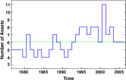
Figure 3: Number of assets without short positions, for FF48. The number of active assets $K_{\mbox{\tiny{pos.}}}$ in $\mathbf{w}^{\mbox{\tiny{pos.}}}$, the optimal portfolio without short positions, from year to year. This number varies from 4 to 11; the average over 30 years is around 6.

Table 1: Performance of the sparse portfolio with no short-selling, for FF48.

Evaluation	$w_{i}\geqslant 0$			Equal
period	for all $i$			weight
	$m$	$\sigma$	$S$	$m$	$\sigma$	$S$
06/76-06/06	17	41	41	17	61	27
07/76-06/81	23	48	49	29	66	44
07/81-06/86	23	41	57	18	58	31
07/86-06/91	9	45	20	5	72	7
07/91-06/96	16	26	62	18	41	44
07/96-06/01	16	40	40	11	67	17
07/01-06/06	13	43	30	18	60	30

Monthly mean return $m$, standard deviation of monthly return $\sigma$, and corresponding Sharpe ratio $S$ (expressed in %) for the optimal no-short-positions portfolio, as well as for the $1/N$-strategy portfolio. Both portfolio strategies are tested for their performance over twelve consecutive months immediately following their construction; their returns are pooled over several years to compute $m$, $\sigma$ and $S$, as described in the text. Statistics reflect the performance an investor would have achieved, on average, by constructing the portfolio on July 1 one year, and keeping it for the next twelve months, until June 30 of the next year, with the average taken over 5 years for each of the break-out periods, over 30 years for the full period.

Figure 4: Outperforming the $1/N$ strategy, for FF48. The Sharpe ratio, for the full period 1976-2006, for several portfolios: $\mathbf{w}^{\mbox{\tiny{pos.}}}$, the optimal portfolio without short positions (red); the portfolios $\mathbf{w}^{K}$ with a fixed number, $K$, of active positions, where $K$ ranges from 11 to 48 (green dots). $\mathbf{w}^{\mbox{\tiny{pos.}}}$ is indicated by a fat solid horizontal red bar, stretching from 4 to 11 (its minimum to maximum number of assets; see also Figure 3.) The binned portfolios $\mathbf{w}^{\mbox{\tiny{bin}}}$ are marked by horizontal blue bars indicating the range of the corresponding bin. The horizontal green line indicates the Sharpe ratio for the $1/N$ portfolio, in which equal amounts are invested in all the assets; a large number of our portfolios significantly outperform this benchmark, with only the least sparse (most weakly penalized) choices underperforming it.

Table 2: Empirical results for FF48.

Evaluation	bin=8-16			bin=17-24			bin=25-32			bin=33-40			bin=41-48			$w_{i}\geqslant 0$
period	$m$	$\sigma$	$S$	m	$\sigma$	$S$	$m$	$\sigma$	$S$	$m$	$\sigma$	$S$	$m$	$\sigma$	$S$	$m$	$\sigma$	$S$
​​07/76-06/06​​	​​16​​	​​40​​	​​40​​	​​14​​	​​40​​	​​34​​	​​12​​	​​43​​	​​28​​	​​12​​	​​47​​	​​26​​	​​12​​	​​54​​	​​22​​	​​17​​	​​41​​	​​41​​
​​07/76-06/81​​	​​20​​	​​41​​	​​50​​	​​18​​	​​39​​	​​46​​	​​19​​	​​40​​	​​49​​	​​22​​	​​43​​	​​50​​	​​23​​	​​50​​	​​46​​	​​23​​	​​48​​	​​49​​
​​07/81-06/86​​	​​25​​	​​42​​	​​58​​	​​23​​	​​44​​	​​52​​	​​24​​	​​46​​	​​52​​	​​23​​	​​50​​	​​46​​	​​22​​	​​56​​	​​39​​	​​23​​	​​41​​	​​57​​
​​07/86-06/91​​	​​8​​	​​43​​	​​18​​	​​7​​	​​44​​	​​15​​	​​4​​	​​47​​	​​9​​	​​4​​	​​51​​	​​7​​	​​5​​	​​57​​	​​8​​	​​9​​	​​45​​	​​20​​
​​07/91-06/96​​	​​15​​	​​26​​	​​57​​	​​13​​	​​27​​	​​47​​	​​12​​	​​33​​	​​36​​	​​12​​	​​41​​	​​30​​	​​11​​	​​52​​	​​21​​	​​16​​	​​26​​	​​62​​
​​07/96-06/01​​	​​16​​	​​41​​	​​38​​	​​9​​	​​42​​	​​22​​	​​3​​	​​50​​	​​6​​	​​2​​	​​54​​	​​4​​	​​0​​	​​61​​	​​0​​	​​16​​	​​40​​	​​40​​
​​07/01-06/06​​	​​13​​	​​42​​	​​30​​	​​12​​	​​41​​	​​29​​	​​10​​	​​38​​	​​28​​	​​10​​	​​37​​	​​27​​	​​12​​	​​43​​	​​27​​	​​13​​	​​43​​	​​30​​

Monthly mean return, $m$, standard deviation of monthly return, $\sigma$, and corresponding monthly Sharpe ratio $S$ (expressed in %) for the optimal portfolios with 8-16, 17-24, 25-32, 33-40, 41-48 assets, as well as (again) the optimal no-short-positions portfolio. Portfolios are constructed annually as described in the text. Statistics reflect the performance an investor would have achieved on average, by constructing the portfolio on July 1 one year, and keeping it for the next twelve months, until June 30 of the next year; the average is taken over several years: 5 for each break-out period, 30 for the full period.

For a “binned” portfolio, such as the 8-to-16 asset portfolio, targeting a narrow range rather than an exact value for the total number of assets, we define the portfolio $\mathbf{w}^{\mbox{\tiny{8-16}}}$ by considering each year the portfolios $\mathbf{w}^{K}$ with $K$ between 8 and 16 (both extremes included), and selecting the one that minimizes the objective function (2); if there are several possibilities, the minimizer with smallest $\ell_{1}$ norm is selected. The results are summarized in Figure 4, which shows the average monthly Sharpe ratio of different portfolios of this type for the entire 30 year exercise. For several portfolio sizes, we are able to significantly outperform the evenly-weighted portfolio (the Sharpe ratio of which is indicated by the horizontal line at 27%). Detailed statistics are reported in Table 2; for comparison, Table 2 lists again the results for the no-short-positions portfolio.

Notice that, according to Table 2, the no-short-positions portfolio outperforms all binned portfolios for the full 30 year period; this is not systematically true for the break-out periods, but even in those break-out periods where it fails to outperform all binned portfolios, its performance is still close to that of the best performing (and sparsest) of the binned portfolios. This observation no longer holds for the portfolio constructions with FF100, our second exercise — see Figure 6 below.

4.2 Example 2: FF100

Except for using a different collection of assets, this exercise is identical in its methodology to what was done for FF48, so that we do not repeat the full details here. Tables 3, 4 and Figures 5, 6 summarize the results; they correspond, respectively, to the results given in Tables 1, 2 and Figures 3, 4 for FF48.

From the results of our two exercises we see that:

• Our sparse portfolios (with a relatively small number of assets and moderate $\tau$) outperform the naïve $1/N$ strategy significantly and consistently over the entire evaluation period. This gain is achieved for a wide range of portfolio sizes, as indicated in Figures 4 and 6. It is to be noted that the best performing sparse portfolio we constructed is not always the no-short-positions portfolio.

• When we target a large number of assets in our portfolio, the performance deteriorates. We interpret this as a result of so-called “overfitting”. Larger target numbers of assets correspond to smaller values of $\tau$. The $\ell_{1}$ penalty is then having only a negligible effect and the minimization focuses essentially on the variance term. Hence, the solution becomes unstable and is overly sensitive to the estimation errors that plague the original (unpenalized) Markowitz optimization problem (2).

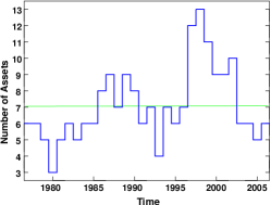
Figure 5: Number of assets without short positions, for FF100. The number of active assets $K_{\mbox{\tiny{pos.}}}$ in $\mathbf{w}^{\mbox{\tiny{pos.}}}$, the optimal portfolio without short positions, from year to year. Note that $K_{\mbox{\tiny{pos.}}}(t)$ is also the minimum value $K_{\mbox{\tiny{min}}}(t)$. For this data set, our construction generates optimal portfolios for all values from $K_{\mbox{\tiny{pos.}}}(t)$ to 60 in every year $t$. $K_{\mbox{\tiny{pos.}}}(t)$ varies from 3 to 13; the average over 30 years is 7.

Table 3: Performance of the sparse portfolio with no short-selling, for FF100.

Evaluation	$w_{i}\geqslant 0$			Equal
period	for all $i$			weight
	$m$	$\sigma$	$S$	$m$	$\sigma$	$S$
06/76-06/06	16	53	30	17	59	28
07/76-06/81	12	59	21	23	61	38
07/81-06/86	24	49	49	20	53	38
07/86-06/91	10	65	15	9	71	13
07/91-06/96	19	31	61	18	34	53
07/96-06/01	18	52	35	16	63	26
07/01-06/06	11	55	21	12	64	19

Monthly mean return $m$, standard deviation of monthly return $\sigma$, and corresponding Sharpe ratio $S$ (expressed in %) for the optimal positive-weights-only portfolio, as well as for the $1/N$-strategy portfolio. Both portfolio strategies are tested for their performance over twelve consecutive months immediately following their construction; their returns are pooled over several years to assess their performance, as described in the text. Statistics reflect the performance an investor would have achieved, on average, by constructing the portfolio on July 1 one year, and keeping it for the next twelve months, until June 30 of the next year; the average is taken over 5 years for each of the break-out periods, over 30 years for the full period.

Table 4: Empirical results for FF100.

Evaluation	bin=11-20			bin=21-30			bin=31-40			bin=41-50			bin=51-60			$w_{i}\geqslant 0$
period	$m$	$\sigma$	$S$	m	$\sigma$	$S$	$m$	$\sigma$	$S$	$m$	$\sigma$	$S$	$m$	$\sigma$	$S$	$m$	$\sigma$	$S$
​​06/76-06/06​​	​​16​​	​​50​​	​​33​​	​​19​​	​​48​​	​​39​​	​​19​​	​​49​​	​​40​​	​​20​​	​​52​​	​​39​​	​​21​​	​​60​​	​​34​​	​​16​​	​​53​​	​​30​​
​​07/76-06/81​​	​​11​​	​​52​​	​​22​​	​​12​​	​​51​​	​​24​​	​​12​​	​​55​​	​​22​​	​​11​​	​​56​​	​​20​​	​​7​​	​​66​​	​​10​​	​​12​​	​​59​​	​​21​​
​​07/81-06/86​​	​​26​​	​​41​​	​​64​​	​​31​​	​​38​​	​​81​​	​​31​​	​​40​​	​​77​​	​​31​​	​​43​​	​​72​​	​​33​​	​​49​​	​​67​​	​​24​​	​​49​​	​​49​​
​​07/86-06/91​​	​​9​​	​​63​​	​​14​​	​​9​​	​​61​​	​​16​​	​​11​​	​​62​​	​​18​​	​​12​​	​​64​​	​​19​​	​​12​​	​​71​​	​​17​​	​​10​​	​​65​​	​​15​​
​​07/91-06/96​​	​​20​​	​​29​​	​​70​​	​​22​​	​​25​​	​​86​​	​​20​​	​​28​​	​​73​​	​​22​​	​​31​​	​​70​​	​​25​​	​​36​​	​​67​​	​​19​​	​​31​​	​​61​​
​​07/96-06/01​​	​​18​​	​​53​​	​​35​​	​​23​​	​​52​​	​​44​​	​​29​​	​​47​​	​​61​​	​​31​​	​​50​​	​​62​​	​​34​​	​​63​​	​​54​​	​​18​​	​​52​​	​​35​​
​​07/01-06/06​​	​​11​​	​​53​​	​​22​​	​​15​​	​​51​​	​​29​​	​​13​​	​​51​​	​​26​​	​​13​​	​​56​​	​​23​​	​​14​​	​​64​​	​​22​​	​​11​​	​​55​​	​​21​​

Monthly mean return, $m$, standard deviation of monthly return, $\sigma$, and corresponding monthly Sharpe ratio $S$ (expressed in %) for the optimal portfolios with 11-20, 21-30, 31-40, 41-50, 51-60 assets, as well as (again) the optimal portfolio without short positions. Portfolios are constructed annually as described in the text. Statistics reflect the performance an investor would have achieved on average, by constructing the portfolio on July 1 one year, and keeping it for the next twelve months, until June 30 of the next year; the average is taken over several years: 5 for each break-out period, 30 for the full period.

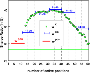
Figure 6: Outperforming the $1/N$ strategy for FF100. The Sharpe ratio, for the full period 1976-2006, for several portfolios: $\mathbf{w}^{\mbox{\tiny{pos.}}}$, the optimal portfolio without short positions (red); the “binned” portfolios $\mathbf{w}^{11-20}$, $\mathbf{w}^{21-30}$, $\mathbf{w}^{31-40}$, $\mathbf{w}^{41-50}$ and $\mathbf{w}^{51-60}$ (blue); and the portfolios $\mathbf{w}^{K}$ with a fixed number, $K$, of active positions, where $K$ ranges from 13 to 60 (green dots circled in black). $\mathbf{w}^{\mbox{\tiny{pos.}}}$ is indicated by a fat solid horizontal red bar, stretching from 3 to 13 (its minimum to maximum number of assets; see also Figure 5.) In this example, optimal sparse portfolios that allow short positions significantly outperform both the evenly-weighted portfolio and the optimal no-short-positions portfolio.

5 Possible generalizations

In this section, we briefly describe some extensions of our approach. It should be pointed out that the relevance and usefulness of the $\ell_{1}$ penalty is not limited to a stable implementation of the usual Markowitz portfolio selection scheme described in Section 2. Indeed, there are several other portfolio construction problems that can be cast in similar terms or otherwise solved through the minimization of a similar objective function. We now list a few examples:

5.1 Partial index tracking

In many situations, investors want to create a portfolio that efficiently tracks an index. In some cases, this will be an existing financial index whose level is tied to a large number of tradable securities but which is not yet tradable en masse as an index future or other single instrument. In such a situation, investors need to find a collection of securities whose profit and loss profile accurately tracks the index level. Such a collection need not be a full replication of the index in question; indeed it is frequently inconvenient or impractical to maintain a full replication.

In other situations, investors will want to monetize some more abstract financial time series: an economic time series, an investor sentiment time series, etc. In that case, investors will need to find a collection of securities which is likely to remain correlated to the target time series.

Either way, the investor will have at his disposal a time series of index returns, which we will write as a $T\times 1$ column vector, $\mathbf{y}$. Also, the investor will have at his disposal the time series of returns for every available security, which we will write as a $T\times N$ matrix $\boldsymbol{R}$, as before.

In that case, an investor seeking to minimize expected tracking error would want to find

$$\widehat{\mathbf{w}}=\arg\min_{\mathbf{w}}\|\mathbf{y}-\boldsymbol{R}\mathbf{w}\|_{2}^{2}.$$

However, this problem is simply a linear regression of the target returns on the returns of the available assets. As the available assets may be collinear, the problem is subject to the same instabilities that we discussed above. As such, we can augment our objective function with an $\ell_{1}$ penalty and seek instead

$$\mathbf{w}^{[\tau]}=\arg\min_{\mathbf{w}}\left[\|\mathbf{y}-\boldsymbol{R}\mathbf{w}\|_{2}^{2}+\tau\|\mathbf{w}\|_{1}\right]~{},$$

subject to the appropriate constraints. This simple modification stabilizes the problem and enforces sparsity, so that the index can be stably replicated with few assets.

Moreover, one can enhance this objective function in light of the interpretation of the $\ell_{1}$ term as a model of transaction costs. Let $s_{i}$ is the transaction cost (bid-ask spread) for the $i$th security. In that case, we can seek

$$\mathbf{w}^{[\tau]}=\arg\min_{\mathbf{w}}\left[\|\mathbf{y}-\boldsymbol{R}\mathbf{w}\|_{2}^{2}+\tau\sum_{i}s_{i}|w_{i}|\right]~{}.$$

By making this modification, the optimization process will “prefer” to invest in more liquid securities (low $s_{i}$) while it will “avoid” investments in less liquid securities (high $s_{i}$). A slightly modified version of the algorithm described above can cope with such weighted $\ell_{1}$ penalty and generate a list of portfolios for a wide range of values for $\tau$. For each portfolio, the investor could then compare the expected tracking error per period ($\frac{1}{\,{}^{\,}T\,}\|\mathbf{y}-\boldsymbol{R}\mathbf{w}\|_{2}^{2}$) with the expected cost of creating and liquidating the tracking portfolio ($\sum_{i}s_{i}|w_{i}|$). The investor could then select a portfolio that suits both his risk tolerance and cost constraints.

5.2 Portfolio hedging

Consider the task of hedging a given portfolio using some subset of a universe of available assets. As a concrete example, imagine trying to efficiently hedge out the market risk in a portfolio of options on a single underlying asset, potentially including many strikes and maturities. An investor would be able to trade the underlying asset as well as any options desired. In this context, it would be possible to completely eliminate market risk by negating the initial position. However, this may not be feasible given liquidity (transaction cost) constraints.

Instead, an investor may simply want to reduce his risk in a cost-efficient way. One could proceed as follows: Generate a list of scenarios. For each scenario, determine the change in the value of the existing portfolio. Also, determine the change in value for a unit of each available security. Store the former in a $M\times 1$ column vector $\mathbf{y}$ and store the latter in a $M\times N$ matrix, $\boldsymbol{X}$. Also, determine a probability, $p_{i}$ for $i=1,\ldots,M$ of each scenario, and store the square root of these values in a diagonal $M\times M$ matrix, $\boldsymbol{P}$. These probabilities can be derived from the market or assumed subjectively according to an investor’s preference. As before, denoting by $s_{i}$ the transaction costs for each tradable security, we can seek

$$\mathbf{w}^{[\tau]}=\arg\min_{\mathbf{w}}\left[\|\boldsymbol{P}\left(\mathbf{y}+\boldsymbol{X}\mathbf{w}\right)\|_{2}^{2}+\tau\sum_{i}s_{i}|w_{i}|\right]~{}.$$

As before, the investor could then apply one of the algorithms above to generate a list of optimal portfolios for a wide range of values of $\tau$. Then, just as in the index tracking case, the investor could observe the attainable combinations of expected mark to market variance ($\|\boldsymbol{P}\left(\mathbf{y}+\boldsymbol{X}\mathbf{w}\right)\|_{2}^{2}$) and transaction cost ($\sum_{i}s_{i}|w_{i}|$). One appealing feature of this method is that it does not explicitly determine the number of assets to be included in the hedge portfolio. The optimization naturally trades off portfolio volatility for transaction cost, rather than imposing an artificial cap on either.

5.3 Portfolio Adjustment

Thus far, we have assumed that investors start with no assets, and must construct a portfolio to perform a particular task. However, this is rarely the case in the real world. Instead, investors frequently hold a large number of securities and must modify their existing holdings to achieve a particular goal. In this context, the investor already holds a portfolio $\mathbf{w}$ and must make an adjustment $\Delta_{\mathbf{w}}$. In that case, the final portfolio will be $\mathbf{w}+\Delta_{\mathbf{w}}$, but the transaction costs will be relevant only for the adjustment $\Delta_{\mathbf{w}}$. The corresponding optimization problems is given by

$$\Delta_{\mathbf{w}}^{[\tau]} = \arg\min_{\Delta_{\mathbf{w}}}\left[\|\rho\mathbf{1}_{T}-\boldsymbol{R}(\mathbf{w}+\Delta_{\mathbf{w}})\|^{2}_{2}+\tau\|\Delta_{\mathbf{w}}\|_{1}\right]$$

s. t. $$\Delta_{\mathbf{w}}^{\top}\widehat{\boldsymbol{\mu}}=0$$

$$\Delta_{\mathbf{w}}^{\top}\mathbf{1}_{N}=0.$$

It is easy to modify our methodology to handle this situation.

6 Conclusion

We have devised a method that constructs stable and sparse portfolios by introducing an $\ell_{1}$ penalty in the Markowitz portfolio optimization. We obtain as special cases the no-short-positions portfolios which also comprise few active assets. To our knowledge, such a sparsity property of the non-negative portfolios has not been previously noticed in the literature. The portfolios we propose can be seen as natural extensions of the no-short-positions portfolios and maintain or improve their performances while preserving as much as possible their sparse nature.

We have also described an efficient algorithm for computing the optimal, sparse portfolios, and we have implemented it using as assets two sets of portfolios constructed by Fama and French: 48 industry portfolios and 100 portfolios formed on size and book-to-market. We found empirical evidence that the optimal sparse portfolios outperform the evenly-weighted portfolios by achieving a smaller variance; moreover they do so with only a small number of active positions, and the effect is observed over a range of values for this number. This shows that adding an $\ell_{1}$ penalty to objective functions is a powerful tool for various portfolio construction tasks. This penalty forces our optimization scheme to select, on the basis of the training data, few assets forming a stable and robust portfolio, rather than being “distracted” by the instabilities due to collinearities and responsible for meaningless artifacts in the presence of estimation errors.

Many variants and improvements are possible on the simple procedure described and illustrated above. This goes beyond the scope of the present paper which was to propose a new methodology and to demonstrate its validity. In future work, we plan to extend our empirical exercises to other and larger asset collections (such as S$\&$P500), to explore other performance criteria than the usual Sharpe ratio, and to derive automatic procedures for choosing the number of assets to be included in our portfolio. We believe that the good regularization properties of our method should ensure its robustness against these various changes.

Appendix: Constrained minimization algorithm

Before discussing our solution method for the linearly constrained $\ell_{1}$-penalized least-squares problem, we briefly recall the homotopy/LARS method which manages to recover the unconstrained minimizer of the $\ell_{1}$-penalized least-squares objective function

$$\bar{\mathbf{w}}(\tau)=\arg\min_{\mathbf{w}}\left[\|\boldsymbol{R}\mathbf{w}-\mathbf{y}\|_{2}^{2}+\tau\|\mathbf{w}\|_{1}\right]$$

for a whole range of values of the (positive) penalty parameter $\tau$.

The variational equations describing the minimizer $\bar{\mathbf{w}}(\tau)$ are:

$$\displaystyle(\boldsymbol{R}^{\top}(\mathbf{y}-\boldsymbol{R}\mathbf{w}))_{i} = \frac{\tau}{2}\,\mathrm{sgn}\,w_{i}\qquad\qquad w_{i}\neq 0$$ (8)

$$\displaystyle|(\boldsymbol{R}^{\top}(\mathbf{y}-\boldsymbol{R}\mathbf{w}))_{i}| \leq \frac{\tau}{2}\qquad\qquad\qquad\,\,\,\,w_{i}=0.$$ (9)

The minimizer $\bar{\mathbf{w}}(\tau)$ is a continuous piecewise linear function of $\tau$. We shall denote the breakpoints by $\tau_{0}>\tau_{1}>\ldots$ and the corresponding minimizers by $\bar{\mathbf{w}}(\tau_{0}),\bar{\mathbf{w}}(\tau_{1}),\ldots$ The breakpoints occur where a new component enters or leaves the support of $\bar{\mathbf{w}}(\tau)$. We will use $\mathbf{b}$ to denote the residual $\mathbf{b}=\boldsymbol{R}^{\top}(\mathbf{y}-\boldsymbol{R}\mathbf{w})$.

The homotopy/LARS method for solving these equations starts by considering the point $\mathbf{w}=0$, which satisfies the equations (8,9) for all $\tau\geq\tau_{0}\equiv 2\max_{i}|(\boldsymbol{R}^{\top}\mathbf{y})_{i}|$. Hence $\bar{\mathbf{w}}(\tau\geq\tau_{0})=0$.

Given a breakpoint $\bar{\mathbf{w}}(\tau_{n})$, it is possible to construct the next breakpoint $\bar{\mathbf{w}}(\tau_{n+1})$ by solving a small linear system. Let $J=\{i\mathrm{\ for\ which\ }\left|\mathbf{b}_{i}\right|=\tau_{n}/2\}$ (i.e. the set of maximal residual), $\boldsymbol{R}_{J}$ the submatrix consisting of the columns $J$ of $\boldsymbol{R}$. We define the walking direction $\mathbf{u}$ by

$$\boldsymbol{R}_{J}^{\top}\boldsymbol{R}_{J}\,\mathbf{u}_{J}=\mathrm{sgn}\left(\mathbf{b}_{J}\right)$$

and $u_{i}=0$ for $i\not\in J$ ($\mathrm{sgn}\left(\mathbf{b}_{J}\right)$ denotes the vector $(\mathrm{sgn}(b_{j})_{j\in J})$). In this way, a step $\mathbf{w}\rightarrow\mathbf{w}+\gamma\mathbf{u}$ results in a change in the residual $\mathbf{b}\rightarrow\mathbf{b}-\gamma\mathbf{v}$, where $v_{j}=\mathrm{sgn}(b_{j})$ for $j\in J$. In other words, the maximal components of the residual decrease at the same rate. The step size $\gamma>0$ is now determined to be the smallest number for which the absolute value of a component $|b_{i}-\gamma v_{i}|$ (with $i\not\in J$) of the new residual becomes equal to $|b_{j}-\gamma v_{j}|$ for $j\in J$ (i.e. a new component joins the maximal residual set), or for which a nonzero component of $\mathbf{w}$ is turned into zero.

The new penalty parameter is then $\tau_{n+1}=\tau_{n}-2\gamma$ (which is smaller than $\tau_{n}$), and the corresponding minimizer is $\bar{\mathbf{w}}(\tau_{n+1})=\bar{\mathbf{w}}(\tau_{n})+\gamma\mathbf{u}$. By construction it is guaranteed to satisfy the variational equations (8,9).

The two main advantages of this method are thus that it is exact (in particular zero components are really zero) and that it yields the breakpoints (and hence the minimizers) for a whole range of values of the penalization parameters $\tau\geq\tau_{\mathrm{stop}}\geq 0$. At each step, only a relatively small linear system has to be solved. If this procedure is carried through until the end, one finds $\lim_{\tau\rightarrow 0}\arg\min\|\boldsymbol{R}\mathbf{w}-\mathbf{y}\|_{2}^{2}+\tau\|\mathbf{w}\|_{1}=\displaystyle\arg\!\!\!\!\!\!\!\!\!\!\!\!\!\min_{\mathbf{w}\ \mathrm{s.t.}\ \boldsymbol{R}^{\top}\boldsymbol{R}\mathbf{w}=\boldsymbol{R}^{\top}\mathbf{y}}\|\mathbf{w}\|_{1}$.

For the constrained case, i.e. the minimization problem

$$\widetilde{\mathbf{w}}(\tau)=\arg\!\!\!\!\!\!\!\!\!\min_{\mathbf{w}\ \mathrm{s.t.}\ \boldsymbol{A}\mathbf{w}=\mathbf{a}}\left[\|\boldsymbol{R}\mathbf{w}-\mathbf{y}\|_{2}^{2}+\tau\|\mathbf{w}\|_{1}\right]$$ (10)

subject to the linear constraint $\boldsymbol{A}\mathbf{w}=\mathbf{a}$, we can devise a similar procedure. We assume, of course, that the constraint $\boldsymbol{A}\mathbf{w}=\mathbf{a}$ has a solution.

An approximation of the minimizer $\widetilde{\mathbf{w}}(\tau)$ can be obtained by applying the unconstrained procedure described above to the objective function

$$\widetilde{\widetilde{\mathbf{w}}}(\tau_{\epsilon})=\arg\min_{\mathbf{w}}\left[\|\boldsymbol{A}\mathbf{w}-\mathbf{a}\|_{2}^{2}+\epsilon\|\boldsymbol{R}\mathbf{w}-\mathbf{y}\|_{2}^{2}+\tau_{\epsilon}\|\mathbf{w}\|_{1}\right].$$ (11)

For sufficiently small $\epsilon$, this will give a good approximation of the constrained minimizer $\widetilde{\mathbf{w}}(\tau)$ corresponding to the penalty $\tau=\tau_{\epsilon}/\epsilon$ (after first going through a number of breakpoints for which $\boldsymbol{A}\mathbf{w}\neq\mathbf{a}$, not even approximately). However, this is clearly an approximate method (often very good) whereas the unconstrained procedure did not involve any approximation.

We solve this issue, and provide an exact method, by solving the minimization problem (11) up to the first order in $\epsilon$. In this approach $\epsilon$ is a small formal positive parameter. Now the minimizer $\widetilde{\widetilde{\mathbf{w}}}(\tau_{\epsilon})$ and $\tau_{\epsilon}$ both depend on $\epsilon$. We can write $\mathbf{w}=\mathbf{w}^{(0)}+\epsilon\mathbf{w}^{(1)}+\mathcal{O}(\epsilon^{2})$ and $\tau_{\epsilon}=\tau^{(0)}+\tau^{(1)}\epsilon+\mathcal{O}(\epsilon^{2})$. We again follow the procedure for the unconstrained method, but take care to use arithmetic (addition, multiplication, comparison, …) up to first order in $\epsilon$.

As before, one starts from $\mathbf{w}=0$, corresponding to a large initial value of $\tau_{\epsilon}$, and follows the path of descending $\tau_{\epsilon}$. The strategy consists of satisfying the variational equations

$$\displaystyle\left(\boldsymbol{A}^{\top}(\mathbf{a}-\boldsymbol{A}\mathbf{w})+\epsilon\boldsymbol{R}^{\top}(\mathbf{y}-\boldsymbol{R}\mathbf{w})\right)_{i} = \frac{\tau_{\epsilon}}{2}\,\mathrm{sgn}\,w_{i}\qquad\qquad w_{i}\neq 0$$ (12)

$$\displaystyle\left|\left(\boldsymbol{A}^{\top}(\mathbf{a}-\boldsymbol{A}\mathbf{w})+\epsilon\boldsymbol{R}^{\top}(\mathbf{y}-\boldsymbol{R}\mathbf{w})\right)_{i}\right| \leq \frac{\tau_{\epsilon}}{2}\qquad\qquad\qquad\,\,\,\,w_{i}=0$$ (13)

at each breakpoint by carefully determining a walking direction $\mathbf{u}=\mathbf{u}^{(0)}+\mathbf{u}^{(1)}\epsilon+\mathcal{O}(\epsilon^{2})$ and a step length $\gamma=\gamma^{(0)}+\gamma^{(1)}\epsilon+\mathcal{O}(\epsilon^{2})$. Using $\mathbf{w}=\mathbf{w}^{(0)}+\epsilon\mathbf{w}^{(1)}+\mathcal{O}(\epsilon^{2})$, we can rewrite equations (12) as

$$\displaystyle\left(\boldsymbol{A}^{\top}(\mathbf{a}-\boldsymbol{A}\mathbf{w}^{(0)})\right)_{i} = \frac{\tau^{(0)}}{2}\,\mathrm{sgn}\,w_{i}$$ (14)

$$\displaystyle\left(-\boldsymbol{A}^{\top}\boldsymbol{A}\mathbf{w}^{(1)}+\boldsymbol{R}^{\top}(\mathbf{y}-\boldsymbol{R}\mathbf{w}^{(0)})\right)_{i} = \frac{\tau^{(1)}}{2}\,\mathrm{sgn}\,w_{i}\ .$$ (15)

From a known breakpoint $\mathbf{w}$ we can proceed to the following breakpoint by a step direction $\mathbf{u}$ and step size $\gamma$ (both depending on $\epsilon$). We again set

$$J=\arg\max_{i}\left|\left(\boldsymbol{A}^{\top}(\mathbf{a}-\boldsymbol{A}\mathbf{w}^{(0)})+\epsilon(-\boldsymbol{A}^{\top}\boldsymbol{A}\mathbf{w}^{(1)}+\boldsymbol{R}^{\top}(\mathbf{y}-\boldsymbol{R}\mathbf{w}^{(0)}))\right)_{i}\right|.$$

As long as $\tau^{(0)}\neq 0$, the components $J$ of $\mathbf{u}$ are determined by

$$\left(\begin{array}[]{cc}\boldsymbol{R}_{J}^{\top}\boldsymbol{R}_{J}&\boldsymbol{A}_{J}^{\top}\boldsymbol{A}_{J}\\ \boldsymbol{A}_{J}^{\top}\boldsymbol{A}_{J}&0\end{array}\right)\left(\begin{array}[]{c}\mathbf{u}_{J}^{(0)}\\ \mathbf{u}_{J}^{(1)}\end{array}\right)=\left(\begin{array}[]{c}0\\ \mathrm{sgn}(\mathbf{b}_{J})\end{array}\right)$$ (16)

and the other components of $\mathbf{u}$ remain zero. The step size $\gamma$ is again determined as before, i.e. when a new component enters the maximal residual set, or when a component leaves the active set. The penalty parameter $\tau_{\epsilon}$ decreases as before: $\tau_{\epsilon}\rightarrow\tau_{\epsilon}-2\gamma$.

At some point in this procedure, $\tau_{\epsilon}$ will become zero in zeroth order: $\tau_{\epsilon}=0+\tau^{(1)}\epsilon+\mathcal{O}(\epsilon^{2})$. The corresponding minimizer (more precisely the zeroth-order part of this breakpoint) will satisfy the constraint $\boldsymbol{A}\mathbf{w}=\mathbf{a}$ and we will have found the first constrained minimizer $\widetilde{\mathbf{w}}$ of (10), corresponding to $\tau_{0}=\tau^{(1)}$ (i.e. the first-order part of the parameter $\tau_{\epsilon}$ of the $\epsilon$-dependent problem at this breakpoint). In the unconstrained case, no such calculations were necessary as the starting point was always equal to $0$. Similarly to the unconstrained case, we have that $\widetilde{\mathbf{w}}(\tau>\tau_{0})=\widetilde{\mathbf{w}}(\tau_{0})$.

In principle, one could continue the $\epsilon$-dependent algorithm, but now that the first breakpoint of $\widetilde{\mathbf{w}}(\tau)$ is determined, it is more advantageous to continue the descent of $\tau$ by introducing Lagrange multipliers $\boldsymbol{\lambda}$ for the problem (10):

$$\widetilde{\mathbf{w}}(\tau)=\arg\!\!\!\!\!\!\!\!\!\!\!\min_{\boldsymbol{\lambda},\,\,\mathbf{w}\ \mathrm{s.t.}\ \boldsymbol{A}\mathbf{w}=\mathbf{a}}\left[\|\boldsymbol{R}\mathbf{w}-\mathbf{y}\|_{2}^{2}+\tau\|\mathbf{w}\|_{1}+2\boldsymbol{\lambda}^{\top}(\boldsymbol{A}\mathbf{w}-\mathbf{a})\right].$$

This minimization problem (analogous to (10)) amounts to solving the equations:

$$\displaystyle(\boldsymbol{R}^{\top}(\mathbf{y}-\boldsymbol{R}\mathbf{w})+\boldsymbol{A}^{\top}\boldsymbol{\lambda})_{i} = \frac{\tau}{2}\,\mathrm{sgn}\,w_{i}\qquad\qquad w_{i}\neq 0$$ (17)

$$\displaystyle|(\boldsymbol{R}^{\top}(\mathbf{y}-\boldsymbol{R}\mathbf{w})+\boldsymbol{A}^{\top}\boldsymbol{\lambda})_{i}| \leq \frac{\tau}{2}\qquad\qquad\qquad\,\,\,\,w_{i}=0$$ (18)

$$\boldsymbol{A}\mathbf{w} = \mathbf{a}.$$ (19)

Equation (17) is the equivalent of equation (15) whereas equation (19) replaces equation (14). We now already have $\tau_{0}$, $\widetilde{\mathbf{w}}(\tau\geq\tau^{(0)})$ and the initial Lagrange multipliers $\boldsymbol{\lambda}=-\boldsymbol{A}\widetilde{\widetilde{\mathbf{w}}}^{(1)}$ (from the first-order part of the last step of the $\epsilon$-dependent problem).

To proceed from one breakpoint to the next ($\mathbf{w}\rightarrow\mathbf{w}+\gamma\mathbf{u}$, and $\boldsymbol{\lambda}\rightarrow\boldsymbol{\lambda}+\gamma\mathbf{s}$ as the multipliers also change), we again need to solve a linear system:

$$\left(\begin{array}[]{cc}\boldsymbol{R}_{J}^{\top}\boldsymbol{R}_{J}&\boldsymbol{A}_{J}^{\top}\\ \boldsymbol{A}_{J}&0\end{array}\right)\left(\begin{array}[]{c}\mathbf{u}_{J}\\ \mathbf{s}\end{array}\right)=\left(\begin{array}[]{c}\mathrm{sgn}(\tilde{\mathbf{b}}_{J})\\ 0\end{array}\right)$$ (20)

with $\tilde{\mathbf{b}}=\boldsymbol{R}^{\top}(\mathbf{y}-\boldsymbol{R}\mathbf{w})+\boldsymbol{A}^{\top}\boldsymbol{\lambda}$. This will guarantee that $\mathbf{w}\rightarrow\mathbf{w}+\gamma\mathbf{u}$ and $\boldsymbol{\lambda}\rightarrow\boldsymbol{\lambda}+\gamma\mathbf{s}$ still satisfy the constraint (19) and the variational equations (17,18). The step size $\gamma$ is determined by the same rule as before: stop when a new component enters the set $J=\arg\max_{i}|(\boldsymbol{R}^{\top}(\mathbf{y}-\boldsymbol{R}\mathbf{w})+\boldsymbol{A}^{\top}\boldsymbol{\lambda})_{i}|$ or when a nonzero component of $\mathbf{w}$ is set to zero. Notice the differences and similarities between the linear systems (20) and (16).

At each breakpoint, this algorithm provides the penalty $\tau_{n}$, the corresponding minimizer $\widetilde{\mathbf{w}}(\tau_{n})$ and the Lagrange multipliers $\boldsymbol{\lambda}_{n}$. Unlike for the unconstrained case, it is now possible that $\widetilde{\mathbf{w}}(\tau)$ remains constant between two breakpoints (i.e. only the Lagrange multipliers $\boldsymbol{\lambda}$ change).

One simplifying assumption (not solved in the homotopy/LARS algorithm) was made in the above description of the algorithm: if the set of maximal residual and the support set differ by more than one component, one should carefully select the correct new components to enter the support. This can be done by using the variational equations, and our implementation handles this case.

One could argue that the starting point (i.e. the first breakpoint) for the constrained minimization problem is simply given by $\widetilde{\mathbf{w}}(\tau_{0})=\displaystyle\arg\!\!\!\!\!\!\!\!\!\min_{\mathbf{w}\ \mathrm{s.t.}\ \boldsymbol{A}\mathbf{w}=\mathbf{a}}\|\mathbf{w}\|_{1}$, which could be calculated by letting the unconstrained solution procedure run its course: $\widetilde{\mathbf{w}}(\tau_{0})=\lim_{\sigma\rightarrow 0}\arg\min_{\mathbf{w}}\left[\|\boldsymbol{A}\mathbf{w}-\mathbf{a}\|_{2}^{2}+\sigma\|\mathbf{w}\|_{1}\right]$. Generically (i.e. excluding special cases), this is correct. However, the problem is that sometimes the minimizer $\arg\!\min_{\mathbf{w}\ \mathrm{s.t.}\ \boldsymbol{A}\mathbf{w}=\mathbf{a}}\|\mathbf{w}\|_{1}$ is not unique. In that case, the starting point for the constrained minimizer is not solely determined by $\boldsymbol{A}$ and $\mathbf{a}$ but also by $\boldsymbol{R}$ and $\mathbf{y}$. In this case, the $\epsilon$-dependent algorithm still chooses the correct starting point from the set $\displaystyle\arg\!\!\!\!\!\!\!\!\min_{\mathbf{w}\ \mathrm{s.t.}\ \boldsymbol{A}\mathbf{w}=\mathbf{a}}\|\mathbf{w}\|_{1}$. This is important to mention because the special constraint $\sum w_{i}=1$ used in this paper, gives rise to such cases.

Our algorithm is well-suited for the portfolio problems discussed in this paper. The size of the matrix, the number of constraints (just two) and, more importantly, the number of nonzero weights in the portfolios are such that a minimization run (i.e. finding the minimizer for a whole range of penalty parameters) can be done in a fraction of a second on a standard desktop.

We calculated the portfolio examples in this paper using both the formal $\epsilon$ approach (in Mathematica) and the approximate small $\epsilon$ approach (in Matlab). The outcomes were always consistent.

References

- (1)
- Bertero and Boccacci (1998) Bertero, M., and P. Boccacci (1998): Introduction to Inverse Problems in Imaging. Institute of Physics Publishing, London.
- Brodie, Daubechies, De Mol, and Giannone (2007) Brodie, J., I. Daubechies, C. De Mol, and D. Giannone (2007): “Sparse and Stable Markowitz portfolios,” Preprint arXiv:0708.0046v1; http://arxiv.org/abs/0708.0046.
- Chen, Donoho, and Saunders (2001) Chen, S. S., D. Donoho, and M. Saunders (2001): “Atomic Decomposition by Basis Pursuit,” SIAM Review, 43, 129–159.
- Daubechies, Defrise, and De Mol (2004) Daubechies, I., M. Defrise, and C. De Mol (2004): “An Iterative Thresholding Algorithm for Linear Inverse Problems With a Sparsity Constraint,” Communications on Pure and Applied Mathematics, 57, 1416–1457.
- De Mol, Giannone, and Reichlin (2006) De Mol, C., D. Giannone, and L. Reichlin (2006): “Forecasting Using a Large Number of Predictors: Is Bayesian Regression a Valid Alternative to Principal Components?,” CEPR Discussion Papers 5829, forthcoming in ”Journal of Econometrics”.
- DeMiguel, Garlappi, Nogales, and Uppal (2007) DeMiguel, V., L. Garlappi, F. J. Nogales, and R. Uppal (2007): “A Generalized Approach to Portfolio Optimization: Improving Performance By Constraining Portfolio Norms,” Preprint July 2007.
- DeMiguel, Garlappi, and Uppal (2007) DeMiguel, V., L. Garlappi, and R. Uppal (2007): “Optimal versus Naive Diversification: How Inefficient Is the 1/N Portfolio Strategy?,” Preprint January 2007, forthcoming in Review of Financial Studies.
- Efron, Hastie, Johnstone, and Tibshirani (2004) Efron, B., T. Hastie, I. Johnstone, and R. Tibshirani (2004): “Least Angle Regression,” Annals of Statistics, 32, 407–499.
- Jagannathan and Ma (2003) Jagannathan, R., and T. Ma (2003): “Risk Reduction in Large Portfolios: Why Imposing the Wrong Constraints Helps,” Journal of Finance, 58(4), 1651–1684.
- Markowitz (1952) Markowitz, H. (1952): “Portfolio Selection,” Journal of Finance, 7, 77–91.
- Osborne, Presnell, and Turlach (2000a) Osborne, M. R., B. Presnell, and B. A. Turlach (2000a): “A New Approach to Variable Selection in Least Squares Problems,” IMA Journal of Numerical Analysis, 20(3), 389–403.
- Osborne, Presnell, and Turlach (2000b) (2000b): “On the LASSO and Its Dual,” Journal of Computational and Graphical Statistics, 9(2), 319–337.
- Tibshirani (1996) Tibshirani, R. (1996): “Regression Shrinkage and Selection via the Lasso,” Journal of the Royal Statistical Society Series B, 58, 267–288.