Theory of spin qubits in nanostructures

Abstract

We review recent advances on the theory of spin qubits in nanostructures. We focus on four selected topics. First, we show how to form spin qubits in the new and promising material graphene. Afterwards, we discuss spin relaxation and decoherence in quantum dots. In particular, we demonstrate how charge fluctations in the surrounding environment cause spin decay via spin–orbit coupling. We then turn to a brief overview of how one can use electron–dipole spin resonance (EDSR) to perform single spin rotations in quantum dots using an oscillating electric field. The final topic we cover is the spin–spin coupling via spin–orbit interaction which is an alternative to the usual spin–spin coupling via the Heisenberg exchange interaction.

1 Introduction

Spin qubits in quantum dot nanostructures (and the underlying physics) is a rapidly evolving research area. After the original proposal [1] based on the electron spin in few electron quantum dots, a number of related research branches have emerged. One of which deals with alternative ways to form spin qubits in solid state devices. Here, the aim is to find spin qubit realizations that either couple only weakly to the environment or that are easy to manipulate. A popular example with a growing interest in the spin qubit community is two-spin qubits (where the spin qubit corresponds to singlet and triplet states of two electrons). [2, 3, 4, 5, 6] Further examples are many-spin cluster qubits composed of antiferromagnetically-coupled spin chains [7, 8] and spin qubits in magnetic molecules. [9, 10] Another active research field is devoted to coherence properties of spin qubits. Here, different aspects of spin relaxation and spin dephasing have been quantitatively analyzed for different dissipation channels. The most dominant ones are spin–orbit interaction, coupling the spin to lattice vibrations [11, 12, 13, 14] and other charge fluctuations [15] as well as the hyperfine interaction of the electron spin with the surrounding nuclear spins. [16, 17, 18, 19, 20, 21]

The success of spin qubits in nanostructures is substantially due to the major experimental breakthroughs that have been achieved in recent years (for recent review articles on spin qubits see Refs. cerle05,coish06,hansrev06). After pioneering experiments on few electron quantum dots [25, 26, 27, 28], a first step towards the realization of quantum computing with the spin of electrons in quantum dots has been made in single-shot measurements of the electron spin. [29, 30, 31] Subsequently, a coherent two-qubit gate (the $\sqrt{{\rm SWAP}}$ gate) has been realized. [3] Recently, coherent single spin rotations have been demonstrated via electron spin resonance techniques using pulsed magnetic fields. [32] Thus, all single- and two-qubit operations required for universal quantum computing have been realized in spin qubits based on the original idea. [1] However, the time scales needed to operate single-qubit gates in spin qubits hosted in lateral quantum dots in GaAs/AlGaAs heterostructures [30, 31, 32] are still quite long as compared to the decoherence time $T_{2}\sim 1-10\mu$s. (Note that this is not the case for two-qubit operations which can be performed as fast as 180 ps for the $\sqrt{{\rm SWAP}}$ gate [3].) The ratio of the operation time and the decoherence time should be of the order of $10^{4}$ to be able to do fault-tolerant quantum computing. The decoherence time is currently limited by the hyperfine interaction of the electron spin with the surrounding nuclear spins [33, 34, 35]. Therefore, it is desirable to form spin qubits in other materials where spin relaxation and spin decoherence are less efficient than in GaAs/AlGaAs heterostructures. Two examples (which have already been realized) are few-electron quantum dots in carbon nanotubes [36, 37, 38, 39] as well as semiconductor nanowires [40, 41]. We discuss below another interesting example, namely spin qubits in graphene, where spin relaxation and spin decoherence mechanisms are expected to be weaker than in GaAs-based devices (for recent review articles on graphene see Refs. castro06,geim07,katsn07).

The article is organized as follows: In Sec. 2, we explain in detail our recent proposal to form spin qubits in graphene quantum dots. Many of the aspects discussed in that section equally apply to spin qubits based on carbon nanotube quantum dots. In Sec. 3, different aspects of spin relaxation and decoherence are reviewed. Afterwards, in Sec. 4, recent ideas to use EDSR to form single spin rotations in quantum dots are discussed. In Sec. 5, we show how spin–spin coupling can be achieved via spin–orbit interaction. Finally, we conclude in Sec. 6.

2 Spin qubits in graphene quantum dots

It is generally believed that carbon-based materials such as nanotubes or graphene are excellent candidates to form spin qubits in quantum dots. This is because spin-orbit coupling is weak in carbon (due to its relatively low atomic weight) [45, 46, 47], and because natural carbon consists predominantly of the zero-spin isotope ¹²C, for which the hyperfine interaction is absent. In this section, we review how to form spin qubits in graphene. [48] A crucial requirement to achieve this goal is to find quantum dot states where the usual valley degeneracy is lifted. We show that this problem can be avoided in quantum dots with so-called armchair boundaries. We furthermore show that spin qubits in graphene can not only be coupled (via Heisenberg exchange) between nearest neighbor quantum dots but also over long distances. This remarkable feature is a direct consequence of the Klein paradox being a distinct property of the quasi-relativistic spectrum of graphene. [49]

Two fundamental problems need to be overcome before graphene can be used to form spin qubits and to operate one or two of them in the standard way. [1, 16] (i) It is difficult to create a tunable quantum dot in graphene because of the absence of a gap in the spectrum. [50, 49]. (ii) Due to the valley degeneracy that exists in graphene [51, 52], it is non-trivial to form two-qubit gates using Heisenberg exchange coupling for spins in neighboring dots. Several attempts have been made to solve the problem (i) [53, 54, 55, 56, 57] (without having problem (ii) in mind). We have recently proposed a setup which solves both problems (i) and (ii) at once. [48] In particular, we assume semiconducting armchair boundary conditions to exist on two opposite edges of the sample. It is known that in such a device the valley degeneracy is lifted [58, 60], which is the essential prerequisite for the appearance of Heisenberg exchange coupling for spins in tunnel-coupled quantum dots, and thus for the use of graphene dots for spin qubits.

We now discuss bound-state solutions in the appropriate setup, which are required for a localized qubit. We first concentrate on a single quantum dot which is assumed to be rectangular with width $W$ and length $L$, see Fig. 1.

Figure 1: (Color online) A ribbon of graphene with semi-conducting armchair boundaries is schematically shown. Two barrier gates (blue) define the rectangular size of the quantum dot (with width $W$ and length $L$). A back gate (red) allows one to shift the energy levels in the dot.

The basic idea of forming the dot is to take a ribbon of graphene with semiconducting armchair boundary conditions in $x$-direction and to electrically confine particles in $y$-direction.

The low energy properties of electrons (with energy $\varepsilon$ with respect to the Dirac point) in such a setup are described by the 4x4 Dirac equation

$$\frac{\hbar v}{i}\begin{pmatrix}\sigma_{x}\partial_{x}+\sigma_{y}\partial_{y}&0\\ 0&-\sigma_{x}\partial_{x}+\sigma_{y}\partial_{y}\end{pmatrix}\Psi+\mu(y)\Psi=\varepsilon\Psi,$$ (1)

where the electric gate potential is assumed to vary stepwise, $\mu(y)=\mu_{\rm gate}$ in the dot region (where $0\leq y\leq L$), and $\mu(y)=\mu_{\rm barrier}$ in the barrier region (where $y<0$ or $y>L$). In Eq. (1), $\sigma_{x}$ and $\sigma_{y}$ are Pauli matrices (denoting the sublattices in graphene). The four component spinor envelope wave function $\Psi=(\Psi^{(K)}_{A},\Psi^{(K)}_{B},-\Psi^{(K^{\prime})}_{A},-\Psi^{(K^{\prime})}_{B})$ varies on scales large compared to the lattice spacing. Here, $A$ and $B$ refer to the two sublattices in the two-dimensional honeycomb lattice of carbon atoms, whereas $K$ and $K^{\prime}$ refer to the vectors in reciprocal space corresponding to the two valleys in the bandstructure of graphene. The appropriate semiconducting armchair boundary conditions for such a wave function can be written as ($\alpha=A,B$) [58]

$$\Psi_{\alpha}^{(K)}|_{x=0} = \Psi_{\alpha}^{(K^{\prime})}|_{x=0},$$

$$\Psi_{\alpha}^{(K)}|_{x=W} = e^{\pm 2\pi/3}\Psi_{\alpha}^{(K^{\prime})}|_{x=W}.$$ (2)

These boundary conditions couple the two valleys and are, thus, the reason why the valley degeneracy is lifted. [59] It is well known that the boundary condition (2) yields the following quantization conditions for the wave vector $k_{x}\equiv q_{n}$ in $x$-direction [58, 60]

$$q_{n}=(n\pm 1/3)\pi/W,\;\;n\in\mathbb{Z}.$$ (3)

The level spacing of the modes (3) can be estimated as $\Delta\varepsilon\approx\hbar v\pi/3W$, which gives $\Delta\varepsilon\sim 30\,{\rm meV}$, where we used that $v\sim 10^{6}\,{\rm m/s}$ and assumed a quantum dot width of about $W\sim 30\,{\rm nm}$. Note that Eq. (3) also determines the energy gap for excitations as $E_{\rm gap}=2\hbar vq_{0}$. Therefore, this gap is of the order of 60 meV, which is unusually small for semiconductors. This is a unique feature of graphene that will allow for long-distance coupling of spin qubits as will be discussed below.

We now present in more detail the ground-state solutions, i.e. $n=0$ in Eq. (3). The corresponding ground-state energy $\varepsilon$ can be expressed relative to the potential barrier $\mu=\mu_{\rm barrier}$ in the regions $y<0$ and $y>L$ as $\varepsilon=\mu_{\rm barrier}\pm\hbar v(q_{0}^{2}+k^{2})^{1/2}$. Here, the $\pm$ sign refers to a conduction band ($+$) and a valence band ($-$) solution to Eq. (1). For bound states to exist and to decay at $y\rightarrow\pm\infty$, we require that $\hbar vq_{0}>|\varepsilon-\mu_{\rm barrier}|$, which implies that the wave vector $k_{y}\equiv k$ in $y$-direction, given by

$$k=i\sqrt{q_{0}^{2}-((\varepsilon-\mu_{\rm barrier})/\hbar v)^{2}},$$ (4)

is purely imaginary. In the dot region ($0\leq y\leq L$), the wave vector $k$ in $y$-direction is replaced by $\tilde{k}$, satisfying $\varepsilon=\mu_{\mathrm{gate}}\pm\hbar v(q_{0}^{2}+\tilde{k}^{2})^{1/2}.$ Again the $\pm$ sign refers to conduction and valence band solutions. (In the following, we focus on conduction band solutions to the problem.) In the energy window

$$|\varepsilon-\mu_{\rm gate}|\geq\hbar vq_{0}>|\varepsilon-\mu_{\rm barrier}|,$$ (5)

the bound state energies are given by the solutions of the transcendental equation

$$\tan(\tilde{k}L)=\frac{\hbar v\tilde{k}\sqrt{(\hbar vq_{0})^{2}-(\varepsilon-\mu_{\rm barrier})^{2}}}{(\varepsilon-\mu_{\rm barrier})(\varepsilon-\mu_{\rm gate})-(\hbar vq_{0})^{2}}.$$ (6)

We show a set of solutions to Eq. (6) for a dot with aspect ratio $q_{0}L=\pi L/3W=5$ in Fig. 2.

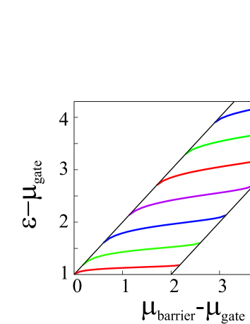
Figure 2: (Color online) Bound-state solutions of a dot with aspect ratio $q_{0}L=\pi L/3W=5$. The diagonal lines indicate the region in which bound-state solutions do exist given by Eq. (5). All energies are taken in units of $\hbar vq_{0}$.

We now turn to the case of two coupled graphene quantum dots, separated by a potential barrier, each dot filled with a single electron. It is interesting to ask whether the spins ${\bf S}_{i}$ of these two electrons ($i=1,2$) are coupled through an exchange coupling, $H_{\rm exch}=J{\bf S}_{1}\cdot{\bf S}_{2}$, in the same way as for regular semiconductor quantum dots [16], because this coupling is, in combination with single-spin rotations, sufficient to generate all quantum gates required for universal quantum computation [1]. The exchange coupling is based on the Pauli exclusion principle which allows for electron hopping between the dots in the spin singlet state (with opposite spins) of two electrons, but not in a spin triplet (with parallel spins), thus leading to a singlet-triplet splitting (exchange energy) $J$.

However, a singlet-triplet splitting $J\neq 0$ only occurs if the triplet state with two electrons on the same dot in the ground state is forbidden, i.e., in the case of a single non-degenerate orbital level. This is a non-trivial requirement in a graphene structure, as in bulk graphene, there is a two-fold orbital degeneracy of states around the points $K$ and $K^{\prime}$ in the first Brillouin zone. This valley degeneracy is lifted in our case of a ribbon with semiconducting armchair edges, and the ground-state solutions determined by Eq. (6) are in fact non-degenerate [62]. The magnitude of the exchange coupling within a Hund-Mulliken model is [16] $J=(-U_{H}+(U_{H}^{2}+16t_{H}^{2})^{1/2})/2+V$, where $t$ is the tunneling (hopping) matrix element between the left and right dot, $U$ is the on-site Coulomb energy, and $V$ is the direct exchange from the long-range (inter-dot) Coulomb interaction. The symbols $t_{H}$ and $U_{H}$ indicate that these quantities are renormalized from the bare values $t$ and $U$ by the inter-dot Coulomb interaction.

For $t\ll U$ and neglecting the long-ranged Coulomb part, this simplifies to the Hubbard model result $J=4t^{2}/U$ where $t$ is the tunneling (hopping) matrix element between the left and right dot and $U$ is the on-site Coulomb energy. In the regime of weak tunneling, we can estimate $t\approx\varepsilon\int\Psi_{L}^{\dagger}(x,y)\Psi_{R}(x,y)dx\,dy$, where $\Psi_{L,R}(x,y)=\Psi(x,y\pm(d+L)/2)$ are the ground-state spinor wave functions of the left and right dots and $\varepsilon$ is the single-particle ground state energy. Note that the overlap integral vanishes if the states on the left and right dot belong to different transverse quantum numbers $q_{n_{L}}\neq q_{n_{R}}$.

For the ground state mode, we have $n_{L}=n_{R}=0$, and the hopping matrix element can be estimated for $d\gtrsim L$ as

$$t\approx 4\varepsilon\alpha_{0}\delta^{*}_{0}Wdz_{0,k}\exp(-d|k|),$$ (7)

where $\alpha_{0}$ and $\delta_{0}$ are wave function amplitudes (with dimension 1/length), see Ref. trau07 for more details. As expected, the exchange coupling decreases exponentially with the barrier thickness, the exponent given by the “forbidden” momentum $k$ in the barrier, defined in Eq. (4).

The values of $t$, $U$, and $J$ can be estimated as follows. The tunneling matrix element $t$ is a fraction of $\varepsilon\sim 30\,{\rm meV}$ (for a width of $W\sim 30\,{\rm nm}$), we obtain that $t\sim 0.5\dots 2.5\,{\rm meV}$. The value for $U$ depends on screening which we can assume to be relatively weak in graphene [52], thus, we estimate, e.g., $U\sim 10\,{\rm meV}$, and obtain $J\sim 0.1\dots 1.5\,{\rm meV}$. (Note that this rough estimate would correspond to very fast switching times $\tau_{s}\sim\hbar/J\sim 1\dots 10$ps for the $\sqrt{{\rm SWAP}}$ operation.)

For the situation with more than two dots in a line, it turns out that we can couple any two of them with the others being decoupled by detuning. In Fig. 3, we illustrate the situation of three dots in a line where the left and the right dot are strongly coupled and the center dot is decoupled by detuning. The tunnel coupling of dot 1 and dot 3 is then achieved via Klein tunneling through the valence band of the two central barriers and the valence band of the center dot. It is important for the long-distance coupling that the exchange coupling of qubit 1 and qubit 3 is primarily achieved via the valence band and not via the qubit level of the center dot – leaving the qubit state of dot 2 unchanged. Using the standard transition matrix approach, we can compare the transition rate of coupling dot 1 and dot 3 via the continuum of states in the valence band of the center dot (which we call $\Gamma_{\rm VB}$) with the transition rate via the detuned qubit level of the center dot (which we call $\Gamma_{\rm QB}$). We obtain for the ratio [48]

$$\Gamma_{\rm VB}/\Gamma_{\rm QB}\approx(L/W)\ln(4\Delta/E_{\rm gap}),$$ (8)

where $\Delta\sim 6\,{\rm eV}$ is the band width of graphene. Therefore, by increasing the aspect ratio $L/W$, it is possible to increase the rate $\Gamma_{\rm VB}$ with respect to $\Gamma_{\rm QB}$. For $L/W=2$ and $E_{\rm gap}\sim 60\,{\rm meV}$, we find that $\Gamma_{\rm VB}/\Gamma_{\rm QB}\sim 12$, meaning that the qubit level in dot 2 is barely used to couple dot 1 and dot 3. This is a unique feature of graphene quantum dots due to the small and highly symmetric band gap.

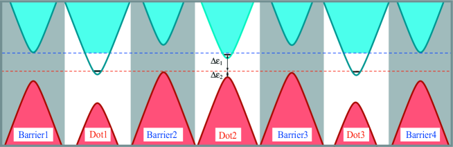
Figure 3: (Color online) The energy bands of a triple quantum dot setup are shown in which dot 1 and dot 3 are strongly coupled via cotunneling processes through the valence bands of barrier 2, barrier 3, and dot 2. The center dot 2 is decoupled by detuning. The energy levels are chosen such that $\Delta\varepsilon_{2}\ll\Delta\varepsilon_{1}$. The triple dot example illustrates that in a line of quantum dots, it is possible to strongly couple any two of them and decouple the others by detuning. This is a unique feature of graphene and cannot be achieved in semiconductors such as GaAs that have a much larger gap (after Ref.[48]) .

3 Spin relaxation and decoherence in quantum dots

Phase coherence of spins in quantum dots (QDs) is of central importance for spin-based quantum computation in the solid state, however, the mechanisms of spin decoherence for extended and localized electrons are rather different. Different mechanisms of spin relaxation in QDs have been considered, such as spin-phonon coupling via spin-orbit (SO) interaction [11, 12, 13, 15] or hyperfine interaction [17], and direct hyperfine coupling [16, 18, 19, 20, 21]. In this section, we consider the spin relaxation and decoherence in quantum dots due to the coupling to phonons and charge fluctuations in the surrounding environment [13, 15]. We show how SO interaction couples the electron spin to these types of fluctuations by deriving an effective Hamiltonian for the spin subspace. Throughout this section, we consider only the leading contribution to SO interaction in two dimensional systems (commonly called linear-in-$p$ SO interaction)

$$H_{SO}=\beta(-p_{x}\sigma_{x}+p_{y}\sigma_{y})+\alpha(p_{x}\sigma_{y}-p_{y}\sigma_{x}),$$ (9)

where $\alpha$ and $\beta$ are Rashba and Dresselhaus coefficients, respectively. Both coefficients have been measured recently in GaAs/InGaAs quantum wells using optical detection schemes. [64] (Note that in this and in the following sections the Pauli matrices denote the electron spin whereas in the previous section it was the sublattice index of graphene.) Moreover, we assume that the temperature is the smallest energy scale in the system and the Zeeman energy is less than the orbital quantization in the QD, $k_{B}T\ll E_{Z}\ll\hbar\omega_{0}$.

Phonon contribution - Lattice vibrations perturb the confining potential $U({\bm{r}})$ of the dot and these fluctuations couple to the electron spin in the QD via the spin–orbit interaction. At low temperatures, the effective Hamiltonian for the electron spin is given by [13]

$$H_{\rm eff} = \frac{1}{2}g\mu_{B}\left[{{\bm{B}}}+\delta{{\bm{B}}}(t)\right]\cdot{{\bm{\sigma}}},$$ (10)

$$\delta{{\bm{B}}}(t) = 2{\bm{B}}\times{\bm{\Omega}}(t),$$ (11)

where ${\bm{B}}$ is the applied magnetic field and ${\bm{\Omega}}(t)$ is the quantum fluctuating field due to the coupling to phonons. Eqs. (10,11) show an important result: In first order in SO interaction, there can be only transverse fluctuations of the effective magnetic field, i.e., $\delta{{\bm{B}}}(t)\cdot{\bm{B}}=0$, and the coupling is proportional to the $B$-field itself. The former property holds true for spin coupling to any fluctuations, be it the noise of a gate voltage or coupling to particle-hole excitations in a Fermi sea. Consequently, there is no pure dephasing and $T_{2}=2T_{1}$ for arbitrarily large Zeeman splitting, in contrast to the naively expected case $T_{2}\ll T_{1}$, where $T_{1}$ is the longitudinal relaxation time (or simply relaxation time) and $T_{2}$ is the transverse relaxation time (decoherence time) of the spin. After averaging over the phonon bath, we find that the spin decay rate has a non-trivial magnetic field dependence; we do not present here the full analytic expression for the magnetic field dependence of the spin decay rate and refer to the original work instead [13]. We plot $1/T_{1}$ as a function of in-plane ${\bm{B}}$ for $\alpha=0$ (only Dresselhaus spin–orbit interaction), see Fig.(4). In agreement with experiment [29], $1/T_{1}$ shows a plateau in a wide range of $B$ fields, due to a crossover from piezoelectric-transverse (dashed curve) to the deformation potential (dot-dashed curve) mechanism of electron-phonon interaction. Note that if $\alpha=\beta$ and ${\bm{B}}\parallel y^{\prime}$ then $1/T_{1}$ vanishes (the same is true for $\alpha=-\beta$ and ${\bm{B}}\parallel x^{\prime}$), where $x^{\prime}\equiv[110]$ and $y^{\prime}\equiv[\bar{1}10]$. A detailed measurement of the $B$-field dependence was reported recently [14] giving very good agreement with theory [13]. Quite remarkably, the largest measured $T_{1}$ times exceed 1 second [14].

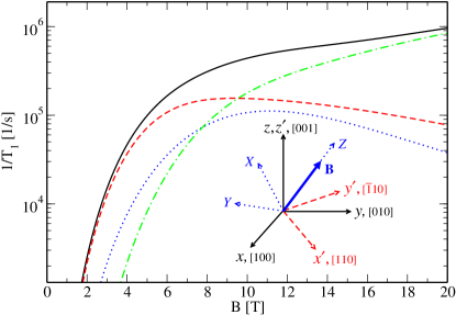
Figure 4: (Color online) Solid curve: The relaxation rate $1/T_{1}$ due to phonons as a function of an in-plane ${\bm{B}}$ for a GaAs QD with $\hbar\omega_{0}=1.1$ meV, $\lambda_{so}=\hbar/m^{*}\beta=1\;\mu$m, and $\alpha=0$. Dashed (dotted) curve: Contribution of the piezoelectric mechanism with transverse (longitudinal) phonons. Dot-dashed curve: Contribution of the deformation potential mechanism. Different coordinate frames are used for the relaxation rate calculations; $(x,y,z)$ are the main crystallographic axes and $(x^{\prime},y^{\prime},z^{\prime})$ are defined as $x^{\prime}=(x+y)/\sqrt{2}$, $y^{\prime}=(y-x)/\sqrt{2}$ and $z^{\prime}=z$.

Quantum point contact (QPC) contribution - Charge fluctuations in the surrounding environment of the QD cause spin decay. Here, we consider one of these sources, a nearby functioning QPC (see Fig.5), in which the charge couples to the spin via spin–orbit interaction in the presence of a magnetic field. The effective Hamiltonian for the electron spin looks the same as Eq.(10), but here, the origin of ${\bm{\Omega}}(t)$ is the electron shot noise in the QPC and its functional dependence on the system parameters is different from the phonon case. There are two mechanisms which contribute to the spin relaxation rate $1/T_{1}$: The electron-hole excitations in the QPC Fermi leads and the electron shot noise in the QPC [15]. In the regime with high bias voltages $\Delta\mu$ applied to the QPC, the latter is the dominant one. To go further, we assume that the applied magnetic field ${\bm{B}}$ is in-plane and along $x^{\prime}$ and we obtain $(E_{Z},T\ll|\Delta\mu\pm E_{Z}|\ll\hbar\omega_{0})$ [15]

$$\frac{1}{T_{1}} \approx \frac{8\pi^{2}e^{2}\hbar^{4}}{{m^{*}}^{2}\kappa^{2}}\frac{\nu^{2}\lambda_{sc}^{4}}{a^{6}\lambda_{+}^{2}}\frac{E_{Z}^{2}\cos^{2}\theta}{(\hbar^{2}\omega_{0}^{2}-E_{Z}^{2})^{2}}S_{LL},$$ (12)

$$S_{LL} = \frac{e^{2}\Delta\mu}{\pi\hbar}{{\cal T}(1-{\cal T})}.$$ (13)

Here $\nu=1/2\pi\hbar v_{F}$ is the density of states per spin and mode in the QPC leads, $m^{*}$ is the electron effective mass, $\kappa$ is the dielectric constant, $a$ is the distance form the QD center to the QPC, $\theta$ is the orientation angle of the QPC on the substrate (see Fig.5), $\lambda_{sc}$ is the Coulomb screening length, $\lambda_{\pm}=\hbar/m^{*}(\beta\pm\alpha)$ are spin-orbit lengths, $\hbar\omega_{0}$ is the orbital quantization energy in the QD, ${\cal T}$ is the transmission coefficient of the QPC, and $S_{LL}$ is the current shot noise. Therefore, in this regime, spin decay rate is linear in bias voltage $\Delta\mu$ and scales as $a^{-6}$. Moreover, $T_{1}$ strongly depends on the QPC orientation on the substrate (the angle $\theta$ between the axes $x^{\prime}$ and $X$, see Fig. (5)), e.g. the non-equilibrium part of the relaxation rate vanishes at $\theta=\pi/2$, for an in-plane magnetic field ${\bm{B}}$ along $x^{\prime}$. We conclude that the spin decay rate can be minimized by tuning certain geometrical parameters of the setup. Our results should also be useful for designing experimental setups such that the spin decoherence can be made negligibly small while charge detection with the QPC is still efficient.

Figure 5: Schematic of the quantum dot (QD) coupled to a QPC. The $(X,Y)$ frame gives the setup orientation, left (L) and right (R) leads, with respect to the crystallographic directions $x^{\prime}\equiv[110]$ and $y^{\prime}\equiv[\bar{1}10]$. The dot has a radius $\lambda_{d}$ and is located at a distance $a$ from the QPC. The vector ${\bm{R}}$ describes the QPC electrons and ${\bm{r}}$ refers to the coordinate of the electron in the dot. The noise of the QPC current $I$ perturbs the electron spin on the dot via the spin–orbit interaction.

4 EDSR in quantum dots

Spin–orbit interaction, although it is one of the main sources of the spin decay in QDs, can be employed to manipulate the electron spin. Here we show how by using an ac electric field together with a static magnetic field, one can coherently rotate the spin of the electron around the Bloch sphere [65]. The physical mechanism responsible for the spin rotation is the so-called EDSR [66] which is similar to usual Electron Spin Resonance (ESR) [67, 68] but, in the former case, the oscillating electric field replaces the oscillating magnetic field in the latter case. The main advantage of EDSR to ESR is its experimental convenience.

We derive an effective Hamiltonian for the electron spin in the presence of a coherent driving ac electric field $V(\mbox{\boldmath$r$},t)=e\int^{\bm{r}}d\mbox{\boldmath$r$}^{\prime}\cdot\mbox{\boldmath$E$}(\mbox{\boldmath$r$}^{\prime},t)\approx e\mbox{\boldmath$E$}(t)\cdot\mbox{\boldmath$r$}$ (see Fig. 6). Hereby, we use the dipole approximation, ignoring the coordinate dependence of the electric field due to the smallness of the dot size compared to the electric field wavelength. This leads us to the following effective spin Hamiltonian [65]

$$H_{\rm eff} = \frac{1}{2}g\mu_{B}{{\bm{B}}}\cdot\mbox{\boldmath$\sigma$}+{1\over 2}{\bm{h}}(t)\cdot\mbox{\boldmath$\sigma$},$$ (14)

$${\bm{h}}(t) = 2g\mu_{B}{\bm{B}}\times\mbox{\boldmath$\Omega$}(t),$$ (15)

$$\mbox{\boldmath$\Omega$}(t) = \frac{-e}{m^{*}\omega_{0}^{2}}\left(\lambda_{-}^{-1}E_{y^{\prime}}(t),\lambda_{+}^{-1}E_{x^{\prime}}(t),0\right),$$ (16)

where ${\bm{E}}(t)={\bm{E}}_{0}\sin{(\omega_{ac}t)}$ of amplitude ${\bm{E}}_{0}=E_{o}(\cos\phi,\sin\phi,0)$ and $\phi$ is the angle of ${\bm{E}}_{0}$ with respect to the axis $x^{\prime}$ (see Fig.6). Note that the resonance happens when $\omega_{ac}=\omega_{Z}=E_{Z}/\hbar$, i.e. when the frequency of the driving field matches the Larmor frequency. The above Hamiltonian has a similar form to the ESR Hamiltonian, except for the fact that the oscillating electric field plays the role of the ac magnetic field. Consequently, we can rotate the electron spin around the Bloch sphere and build a universal single qubit gate. However, to quantify the efficiency of our EDSR scheme, we need to estimate the amplitude of the EDSR field, ${\bm{h}}(t)$, which is proportional to the Rabi frequency $\omega_{R}$. For GaAs QDs, we assume that $\lambda_{+}\approx\lambda_{-}\approx\lambda_{SO}=8\,\mu{\rm m}$, $|g|=0.44$, $\hbar\omega_{0}=1\,{\rm meV}$, and $E_{0}=10^{2}\,{\rm V}/{\rm cm}$, which yields $|{\bm{\Omega}}|\sim 10^{-3}$. Together with the applied magnetic field $B=10\,{\rm T}$, we obtain $\omega_{R}\sim 10^{8}\,{\rm s}^{-1}$. We conclude that, with the present QD setups, EDSR enables one to manipulate the electron spin on a time scale of $10$ ns, which is considerably shorter than typical spin dephasing times $T_{2}\sim 1-10\mu$s in gated GaAs QDs. This mechanism has recently been employed to experimentally rotate the electron spin in quantum dots [69] with $\pi/2$ rotations as fast as $\sim 55$ns. In a similar experimental setup, hyperfine-mediated gate-driven electron spin resonance has been observed. [70]

Up to now, we have only considered the linear-in-$p$ spin–orbit interaction. However, if the two dimensional electron gas (2DEG) has a finite width $d$, then the so-called $p^{3}$ terms of the Dresselhaus spin–orbit interaction also come into the play:

$$H_{SO}=\frac{\gamma}{2}\left(p_{y}p_{x}p_{y}\sigma_{x}-p_{x}p_{y}p_{x}\sigma_{y}\right),$$ (17)

where $\gamma=\alpha_{c}/\sqrt{2{m^{*}}^{3}E_{g}}$ is the spin-orbit coupling constant, with $\alpha_{c}$ ($\sim 0.07$ for GaAs), and $E_{g}$ the band gap. Quite remarkably, if the quantum dot potential is harmonic, then the spin does not couple to $\mbox{\boldmath$E$}(t)$ in the first order of $H_{SO}$ and zeroth order of $E_{Z}$ [65]. Thus, for a harmonic confining potential, one is left with the same dominant mechanism as considered above for the ”linear in $p$” terms. To estimate the strength of the resulting EDSR, we expand in terms of the Zeeman interaction and note that $\gamma\sim\beta d^{2}/\hbar^{2}$, and therefore the amplitude of $\mbox{\boldmath$h$}(t)=2g\mu_{B}{\bm{B}}\times\mbox{\boldmath$\Omega$}(t)$ is by a factor $d^{2}/\lambda_{d}^{2}\ll 1$ smaller as compared to the corresponding amplitude of the linear-in-$p$ contributions.

Next we consider a quantum dot with anharmonic potential $U({\bm{r}})$ and show that the $p^{3}$-terms in Eq. (17) give rise to a spin-electric coupling proportional to the cyclotron frequency $\omega_{c}=eB_{z}/m^{*}c$. [65] Since $\hbar\omega_{c}$ differs parametrically from $E_{Z}$ ($E_{Z}/\hbar\omega_{c}=gm^{*}B/2mB_{z}$), the $p^{3}$-terms can be as significant as the $p$-terms, provided $E_{Z}/\hbar\omega_{c}\lesssim d^{2}/\lambda^{2}$, which is realistic for GaAs quantum dots. As an example, we consider $U(r)=m^{*}\omega_{0}^{2}r^{2}/2\;+\;\eta r^{4}$ , where $\eta$ is a measure of deformation from a harmonic confinement, and obtain [65]

$$\frac{1}{2}{\bm{h}}(t)\cdot\mbox{\boldmath$\sigma$}=\frac{e\gamma\eta\hbar^{2}\omega_{c}}{9m^{*}\omega_{0}^{4}}\left(E_{y}(t)\sigma_{x}+E_{x}(t)\sigma_{y}\right).$$ (18)

Finally, we note that the $p^{3}$-terms can also be relevant for spin relaxation in quantum dots with anharmonic confining potential. Of course, the magnetic field has to have an out-of-plane component for this spin-electric coupling to dominate over the one considered in the previous section.

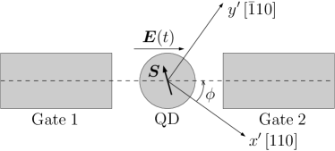
Figure 6: Setup for electric field control of spin via the spin–orbit interaction. The quantum dot (QD) contains a single electron with spin $\mbox{\boldmath$S$}=(\hbar/2)\mbox{\boldmath$\sigma$}$, deep in the Coulomb blockade valley, and in the presence of an external static magnetic field giving rise to a Zeeman splitting $E_{Z}$. The gates $1$ and $2$ are used to generate an alternating electric field $\mbox{\boldmath$E$}(t)$, which acts via the spin–orbit interaction on the electron spin. As a result, an electric dipole spin resonance (EDSR) occurs if the frequency of $\mbox{\boldmath$E$}(t)$ is tuned to match the Larmor frequency $\omega_{Z}=E_{Z}/\hbar$.

5 Spin–spin coupling via spin–orbit interaction

In this part of the article, we discuss the interaction of two electron spins localized in quantum dots through the combined effect of spin–orbit interaction and Coulomb repulsion. The two single-electron quantum dot system is shown in Fig. 7. It is assumed that the two dots are well separated from each other such that there is no electron tunneling between them. In this respect, the interaction between the spins is fundamentally different from the Heisenberg exchange interaction for which the presence of tunneling is crucial[16]. Similarly, the combined effect of Heisenberg exchange interaction and spin-orbit coupling[71, 72, 73, 74, 75]is also based on tunneling and should be carefully distinguished from the spin-orbit effect studied here. Even though the Heisenberg exchange coupling allows typically for much stronger spin-spin coupling than the electrostatically induced one[76], the latter one can prove useful for cases where it is difficult to get sufficient wavefunction overlap (needed for large Heisenberg exchange), and, moreover, it is also important to understand in detail the electrostatically induced spin–spin coupling in order to get control over possible interference effects between different types of coupling. This will be of importance for spin–qubit applications in order to minimize spin decoherence and gate errors.

We give now a short theoretical description of our system. The Hamiltonian of the two-single electron quantum dot system is

$$H=\sum_{i=1,2}\left(\frac{p_{i}^{2}}{2m^{*}}+U(r_{i})+\frac{1}{2}g\mu_{B}\bm{B}\cdot\bm{\sigma}_{i}+H_{SO}^{i}\right)+\frac{e^{2}}{\kappa|\bm{r}_{1}-\bm{r}_{2}+\bm{a}_{0}|},$$ (19)

where the first two terms are the kinetic and orbital confinement ($U(r_{i})=m^{*}\omega_{0}^{2}r_{i}^{2}/2$), the third term is the Zeeman energy, the fourth term stands for the spin–orbit interaction, both Rashba and Dresselhaus [see Eq. (9)], while the last term stands for the Coulomb coupling between the two electrons. The distance between the centers of the two dots is $a_{0}$. Usually, the spin–orbit interaction is a weak perturbation compared with the orbital level spacing and as a consequence can be treated within perturbation theory, as it was done also in the two previous sections. However, here we have an additional energy scale given by the strength of the Coulomb repulsion. This strength is measured through the parameter $\delta=(\lambda/a_{B})(\lambda/a_{0})$[76], where $\lambda=\sqrt{\hbar/m^{*}\omega_{0}}$ is the dot radius and $a_{B}=\hbar^{2}\kappa/m^{*}e^{2}$ is the Bohr radius in the material. In the general case of arbitrary strong Coulomb repulsion, the effective spin Hamiltonian $H_{spin}$ of the two electron system reads[76]

$$H_{spin}=\frac{1}{2}E_{1Z}^{{\it eff}}\sigma_{z}^{1}+\frac{1}{2}E_{2Z}^{{\it eff}}\sigma_{z}^{2}+J_{x}\sigma_{x}^{1}\sigma_{x}^{2}+J_{y}\sigma_{y}^{1}\sigma_{y}^{2},$$ (20)

where the explicit expressions for the spin-orbit renormalized Zeeman splittings $E_{iZ}^{{\it eff}}$ and spin-spin couplings $J_{x,y}$ are given in Ref. trif2007. This interaction vanishes for vanishing Zeeman splitting and is highly anisotropic (XY type). Due to the finite Zeeman splitting, the relevant electrostatically induced spin-spin coupling can be written as

$$H_{s-s}=J_{{\it eff}}(\sigma_{+}^{1}\sigma_{-}^{2}+\sigma_{+}^{2}\sigma_{-}^{1}),$$ (21)

with $\sigma_{\pm}=\sigma_{x}\pm i\sigma_{y}$ and $J_{{\it eff}}=(1/2)(J_{x}+J_{y})$[76]. Up to now we posed no assumptions on the strength of the Coulomb repulsion. However, there are two interesting limiting cases, namely $\delta\ll 1$ (weak Coulomb repulsion) and $\delta\gg 1$ (strong Coulomb repulsion).

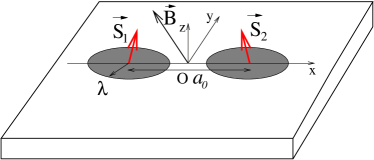
Figure 7: (Color online) The figure shows a sketch of the model system which consists of two identical quantum dots in the $xy$-plane, separated by distance $a_{0}$ (measured from dot-center to dot-center). $\vec{S}_{i}$ denotes the spin of electron $i=1,2$, $\lambda$ is the dot radius, and $\vec{B}$ is the external magnetic field. The respective orbital wave functions of electron 1 and 2 are assumed to have no overlap (i.e. tunneling between the dots is excluded). The remaining purely electrostatic Coulomb interaction between the electron charges leads, via spin–orbit interaction, to an effective coupling between their spins. This spin-spin interaction depends sensitively on the orientation of $\vec{B}$, with no component along it, and is proportional to $\vec{B}^{2}$.

In the first case, $\delta\ll 1$, the Coulomb interaction is a weak perturbation compared to the bare orbital level spacing $\hbar\omega_{0}$ such that

$$H_{s-s}=\int d\bm{r}_{1}d\bm{r}_{2}\frac{\delta\rho_{1}\delta\rho_{2}}{\kappa|\bm{r}_{1}-\bm{r}_{2}+\bm{a}_{0}|}.$$ (22)

Here, the 2x2 matrices $\delta\rho_{1,2}$ are the spin-orbit induced charge distributions or spin-dependent charge distributions in each dot in the absence of Coulomb interaction[76]. From Eq. (22) we see that the spin-spin interaction results from a Coulomb-type coupling between two charge distributions which themselves depend on spin. In the limit of large interdot distances $a_{0}\gg\lambda$, we can perform a multipolar expansion, such that within the lowest order we obtain

$$H_{s-s}\approx\frac{\bm{m}_{1}\cdot\bm{m}_{2}-3(\bm{m}_{1}\cdot\bm{n}_{a})(\bm{m}_{2}\cdot\bm{n}_{a})}{\kappa a_{0}^{3}}$$ (23)

where $\bm{n}_{a}=\bm{a}_{0}/a_{0}$. The dipole moments $\bm{m}_{i}=\langle 0|\delta\rho_{i}\bm{r}_{i}|0\rangle\equiv\bar{\bar{\mu}}\bm{\sigma}_{i}$, where $|0\rangle$ is the orbital ground-state and $\bar{\bar{\mu}}$ is the tensor corresponding to an effective spin-orbit magneton (for explicit expressions see Ref. trif2007). The strength of this effective spin-orbit induced magneton is given by $||\bar{\bar{\mu}}||\approx eE_{Z}/m^{*}\omega_{0}^{2}\lambda_{SO}$. To give an estimate, we assume $\hbar\omega_{0}\sim 0.5\,{\rm meV}$, $E_{Z}\sim 0.05\,{\rm meV}$ ($B\sim 2\,{\rm T}$) and $m^{*}=0.067m_{e}$, $\lambda_{SO}\sim 10^{-6}\,{\rm m}$ for GaAs quantum dots which gives, when compared with the Bohr magneton, $||\bar{\bar{\mu}}||/\mu_{B}\sim 10^{3}$. This implies that the spin-orbit induced dipole-dipole interaction in Eq. (23) can be much stronger than the direct dipole-dipole interaction in vacuum, whose strength is given by $\mu_{B}$. Also, still in the limit $\delta\ll 1$, but for arbitrary interdot distance $a_{0}$ the effective coupling $J_{{\it eff}}$ has the form

$$J_{{\it eff}}=E_{Z}\frac{\lambda}{a_{B}}\frac{E_{Z}}{\hbar\omega_{0}}\left(\frac{\lambda}{\lambda_{SO}}\right)^{2}G(a_{0}/\lambda,\theta,\Phi),$$ (24)

where the function $G(a_{0}/\lambda,\theta,\Phi)$ is plotted in Fig. 8 as a function of $a_{0}/\lambda$ for different angles $\theta,\Phi$. The key feature of the electrostatic spin-spin interaction is that it can range from ferromagnetic to antiferromagnetic type, depending on the magnetic field orientation, passing even through zero for certain angles and/or inter-dot distances.

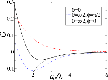
Figure 8: (Color online) The function $G$ occurring in Eq. (24) plotted as a function of the geometric distance $a_{0}$ between the dot centers scaled by the dot radius $\lambda$ for different magnetic field orientations. The dashed line represents the dipolar approximation of $G$ for a perpendicular magnetic field ($\theta=0$) which scales like $a_{0}^{-3}$.

We now focus on the opposite limit $\delta\gg 1$, when the Coulomb interaction is much stronger than the bare orbital level spacing $\hbar\omega_{0}$. Then, we approximate $e^{2}/\kappa|\bm{r}+\bm{a}_{0}|\rightarrow(e^{2}/2\kappa a^{3})[3(\bm{n}_{a}\cdot\bm{r})^{2}-r^{2}]$[76], where $a$ is the effective distance between the electrons due to the combined effect of Coulomb repulsion and orbital confinement. For the explicit derivation of the effective distance $a$ in terms of the bare one $a_{0}$ see Ref. trif2007. Within this ansatz, the spin-spin coupling Hamiltonian takes the form

$$H_{s}=\frac{E_{Z}^{2}}{m^{*2}\omega_{0}^{2}\lambda_{SO}^{2}}\left[\left(\frac{1}{b_{x}^{2}}-1\right)\sigma_{x}^{1}\sigma_{x}^{2}+\left(\frac{1}{b_{y}^{2}}-1\right)\sigma_{y}^{1}\sigma_{y}^{2}\right]$$ (25)

for the case of a perpendicular magnetic field. In the above expression we have $b_{x}=\sqrt{1+4(\lambda/a_{B})(\lambda/a)^{3}}$ and $b_{y}=\sqrt{1-2(\lambda/a_{B})(\lambda/a)^{3}}$.

Let us give now some estimates for the coupling $J_{{\it eff}}$ when an in-plane magnetic field is applied along, say, the $x$-direction. Assuming now GaAs quantum dots, and $E_{Z}=0.1\;{\rm meV}$ ($B=4{\rm\;T}$), $\hbar\omega_{0}=0.5\;{\rm meV}$ ($\lambda/a_{B}\sim 5$), $\lambda/\lambda_{SO}\sim 10^{-1}$. Using these numbers and taking for the geometric inter-dot distance $a_{0}/\lambda\sim 2$, we obtain $J_{{\it eff}}\sim 10^{-7}\;{\rm eV}$. It is worth mentioning that the hyperfine interaction between the electron and the collection of nuclei in a quantum dot ($\sim 10^{5}$) leads to similar energy scales[18, 20]. This shows that the spin-spin coupling derived here can be very relevant for the spin dynamics in the case of electrostatically coupled quantum dots and that it can also compete with other types of interactions. Considering now the case of InAs quantum dots [40, 41] in a magnetic field along the $x$ direction, with $\lambda_{SO}\sim 2\lambda\sim 100{\rm nm}$ and $E_{Z}/\hbar\omega_{0}=0.1$ and taking also $a_{0}/\lambda\sim 2$, a value of $J_{{\it eff}}\sim 10^{-6}{\rm eV}$ is obtained.

6 Conclusions

We have discussed several selected topics on the theory of spin qubits in nanostructures. We have first reviewed our recent proposal how to form spin qubits in graphene. This is interesting for two reasons. On the one hand, one expects very long spin lifetimes in graphene because of a weak spin–orbit interaction and very few host atoms with a nuclear spin. On the other hand, spin qubits in graphene allow for a new type of long distance coupling that uses the property that a ribbon of graphene is a small bandgap semiconductor. Furthermore, we have pointed out several aspects of spin relaxation and decoherence due to spin–orbit interaction and the coupling to a bath. As two possible dissipation channels we have considered lattice vibrations (phonons) and charge fluctuations in the surrounding environment, for instance, a nearby quantum point contact. Subsequently, we have shown how to use EDSR to rotate the spin of an electron in a quantum dot using an oscillating electric field (instead of the oscillating magnetic field employed in the usual ESR). In the final part of the review article, we have discussed how to couple two spins (located in two different quantum dots) via spin–orbit interaction in a situation in which direct tunneling between the dots is highly suppressed.

We would like to thank D.V. Bulaev, G. Burkard, and V.N. Golovach for the collaboration on the work reviewed in this article. Financial support has been provided by the Swiss NSF, the NCCR Nanoscience, and JST ICORP.

References

- [1] D. Loss and D.P. DiVincenzo, Phys. Rev. A57, 120 (1998).
- [2] J. Levy, Phys. Rev. Lett.89, 147902 (2002).
- [3] J. R. Petta, A. C. Johnson, J. M. Taylor, E. A. Laird, A. Yacoby, M. D. Lukin, C. M. Marcus, M. P. Hanson, and A. C. Gossard, Science 309, 2180 (2005).
- [4] J. M. Taylor, W. Dür, P. Zoller, A. Yacoby, C. M. Marcus, and M. D. Lukin, Phys. Rev. Lett.94, 236803 (2005).
- [5] G. Burkard and A. Imamoglu, Phys. Rev. B74, 041307 (2006).
- [6] R. Hanson and G. Burkard, Phys. Rev. Lett.98, 050502 (2007).
- [7] F. Meier, J. Levy, and D. Loss, Phys. Rev. Lett.90, 047901 (2003).
- [8] F. Meier, J. Levy, and D. Loss, Phys. Rev. B68, 134417 (2003).
- [9] M.N. Leuenberger and D. Loss, Nature 410, 789 (2001).
- [10] J. Lehmann, A. Gaita-Arino, E. Coronado, and D. Loss, Nature Nano. 2, 312 (2007).
- [11] A.V. Khaetskii and Y.V. Nazarov, Phys. Rev. B61, 12639 (2000).
- [12] A.V. Khaetskii and Y.V. Nazarov, Phys. Rev. B64, 125316 (2001).
- [13] V.N. Golovach, A.V. Khaetskii, and D. Loss, Phys. Rev. Lett.93, 016601 (2004).
- [14] S. Amasha, K. MacLean, I. Radu, D.M. Zumbühl, M.A. Kastner, M.P. Hanson, and A.C. Gossard, arXiv:cond-mat/0607110.
- [15] M. Borhani, V.N. Golovach, and D. Loss, Phys. Rev. B 73, 155311 (2006).
- [16] G. Burkard, D. Loss, and D.P. DiVincenzo, Phys. Rev. B59, 2070 (1999).
- [17] S.I. Erlingsson, Y.V. Nazarov, and V.I. Fal’ko, Phys. Rev. B64, 195306 (2001).
- [18] A.V. Khaetskii, D. Loss, and L. Glazman, Phys. Rev. Lett.88, 186802 (2002).
- [19] I.A. Merkulov, Al.L. Efros, and M. Rosen, Phys. Rev. B 65, 205309 (2002).
- [20] W.A. Coish and D. Loss, Phys. Rev. B70, 195340 (2004).
- [21] D. Klauser, W.A. Coish, and D. Loss, Phys. Rev. B73, 205302 (2006).
- [22] V. Cerletti, W.A. Coish, O. Gywat, and D. Loss, Nanotechnology 16, R27 (2005).
- [23] W.A. Coish and D. Loss, to appear in Handbook of Magnetism and Advanced Magnetic Materials, vol. 5, Wiley; arXiv:cond-mat/0606550.
- [24] R. Hanson, L.P. Kouwenhoven, J.R. Petta, S. Tarucha, and L.M.K. Vandersypen, to appear in Rev. Mod. Phys.; arXiv:cond-mat/0610433.
- [25] S. Tarucha, D.G. Austing, T. Honda, R.J. van der Hage, and L.P. Kouwenhoven, Phys. Rev. Lett.77, 3613 (1996).
- [26] K. Ono, D.G. Austing, Y. Tokura, and S. Tarucha, Science 297, 1313 (2002).
- [27] T. Fujisawa, D.G. Austing, Y. Tokura, Y. Hirayama, and S. Tarucha, Nature 419, 278 (2002).
- [28] T. Hayashi, T. Fujisawa, H.D. Cheong, Y.H. Jeong, and Y. Hirayama, Phys. Rev. Lett.91, 226804 (2003).
- [29] R. Hanson, B. Witkamp, L.M.K. Vandersypen, L.H. Willems van Beveren, J.M. Elzerman, and L.P. Kouwenhoven, Phys. Rev. Lett. 91, 196802 (2003).
- [30] J.M. Elzerman, R. Hanson, L.H. Willems van Beveren, B. Witkamp, L.M.K. Vandersypen, and L.P. Kouwenhoven, Nature 430, 431 (2004).
- [31] R. Hanson, L.H. Willems van Beveren, I.T. Vink, J.M. Elzerman, W.J.M. Naber, F.H.L. Koppens, L.P. Kouwenhoven, and L.M.K. Vandersypen, Phys. Rev. Lett.94, 196802 (2005).
- [32] F.H.L. Koppens, C. Buizert, K.J. Tielrooij, I.T. Vink, K.C. Nowack, T. Meunier, L.P. Kouwenhoven, and L.M.K. Vandersypen, Nature 442, 766 (2006).
- [33] K. Ono and S. Tarucha, Phys. Rev. Lett.92, 256803 (2004).
- [34] A.C. Johnson, J.R. Petta, J.M. Taylor, A. Yacoby, M. Lukin, C.M. Marcus, M.P. Hanson, and A.C. Gossard, Nature 435, 925 (2005).
- [35] F.H.L. Koppens, J.A. Folk, J.M. Elzerman, R. Hanson, L.H. Willems van Beveren, I.T. Vink, H.P. Tranitz, W. Wegscheider, L.P. Kouwenhoven, and L.M.K. Vandersypen, Science 309, 1346 (2005).
- [36] N. Mason, M.J. Biercuk, and C.M. Marcus, Science 303, 655 (2004).
- [37] M. Biercuk, S. Garaj, N. Mason, J. Chow, and C.M. Marcus, Nano Lett. 5, 1267 (2005).
- [38] S. Sapmaz, C. Meyer, P. Beliczynski, P. Jarillo-Herrero, and L.P. Kouwenhoven, Nano Lett. 6, 1350 (2006).
- [39] M.R. Gräber, W.A. Coish, C. Hoffmann, M. Weiss, J. Furer, S. Oberholzer, D. Loss, and C. Schönenberger, Phys. Rev. B 74, 075427 (2006).
- [40] C. Fasth, A. Fuhrer, M. Bjork, and L. Samuelson, Nano Lett. 5, 1487 (2005).
- [41] A. Pfund, I. Shorubalko, K. Ensslin, and R. Leturcq, Phys. Rev. Lett.99, 036801 (2007).
- [42] A.H. Castro Neto, F. Guinea, and N.M.R. Peres, Physics World, November, 33 (2006).
- [43] A.K. Geim and K.S. Novoselov, Nature Mat. 6, 183 (2007).
- [44] M.I. Katsnelson, Materials Today 10, 20 (2007).
- [45] T. Ando, J. Phys. Soc. Jpn. 6, 1757 (2000).
- [46] H. Min, J.E. Hill, N.A. Sinitsyn, B.R. Sahu, L. Kleinman, and A.H. MacDonald, Phys. Rev. B74, 165310 (2006).
- [47] D. Huertas-Hernando, F. Guinea, and A. Brataas, Phys. Rev. B74, 155426 (2006).
- [48] B. Trauzettel, D.V. Bulaev, D. Loss, and G. Burkard, Nature Phys. 3, 192 (2007).
- [49] M.I. Katsnelson, K.S. Novoselov, and A.K. Geim, Nature Phys. 2, 620 (2006).
- [50] V.V. Cheianov and V.I. Falko, Phys. Rev. B74, 041403(R) (2006).
- [51] G.W. Semenoff, Phys. Rev. Lett.53, 2449 (1984).
- [52] D.P. DiVincenzo and E.J. Mele, Phys. Rev. B29, 1685 (1984).
- [53] J. Nilsson, A.H. Castro Neto, F. Guinea, and N.M.R. Peres, arXiv:cond-mat/0610290.
- [54] P.G. Silvestrov and K.B. Efetov, Phys. Rev. Lett.98, 016802 (2007).
- [55] A. De Martino, L. Dell’Anna, and R. Egger, Phys. Rev. Lett.98 066802 (2007).
- [56] J. Milton Pereira Jr., P. Vasilopoulos, and F.M. Peeters, Nano Lett. 7, 946 (2007).
- [57] T. Stauber, N.M.R. Peres, and F. Guinea, arXiv:0707.3004.
- [58] L. Brey and H.A. Fertig, Phys. Rev. B73, 235411 (2006).
- [59] In Eq. (2), the semiconducting armchair boundary conditions are formulated in a slightly different way than in Ref. \citeonlinebrey06 which is due to a different definition of the width of a ribbon of graphene. In Ref. \citeonlinebrey06, the width is defined as the distance from one outer edge of the armchair boundary to the other outer edge of the armchair boundary (on the other side of the ribbon). In Ref. \citeonlinetrau07 (and also in Ref. \citeonlinetwor06) instead, the width is defined as the distance from one inner edge of the armchair boundary to the other inner edge of the armchair boundary (on the other side of the ribbon). These boundary conditions are fully consistent with each other and with an earlier tight-binding model analysis of the spectrum of graphene nanoribbons. [61]
- [60] J. Tworzydlo, B. Trauzettel, M. Titov, A. Rycerz, and C.W.J. Beenakker, Phys. Rev. Lett.96, 246802 (2006).
- [61] K. Nakada, M. Fujita, G. Dresselhaus, and M.S. Dresselhaus, Phys. Rev. B54, 17954 (1996).
- [62] An alternative way to lift the valley degeneracy in graphene (which does not rely on special boundary conditions) is to form quantum dots in ring structures and to apply a magnetic field perpendicular to the surface of graphene, see Ref. \citeonlinerecher.
- [63] P. Recher, B. Trauzettel, Ya.M. Blanter, C.W.J. Beenakker, and A.F. Morpurgo, arXiv:0706.2103.
- [64] L. Meier, G. Salis, I. Shorubalko, E. Gini, S. Schön, and K. Ensslin, Nature Phys., 15 July 2007, doi:10.1038/nphys675.
- [65] V.N. Golovach, M. Borhani, and D. Loss, Phys. Rev. B 74, 165319 (2006).
- [66] E.I. Rashba and V.I. Sheka, Landau Level Spectroscopy (North-Holland, Amsterdam, 1991).
- [67] N.M. Atherton, Electron Spin Resonance (Ellis Horwod Limited, New York, 1973).
- [68] H.-A. Engel and D. Loss, Phys. Rev. Lett.86, 4648 (2001); Phys. Rev. B65, 195321 (2002).
- [69] K.C. Nowack, F.H.L. Koppens, Yu.V. Nazarov, and L.M.K. Vandersypen, arXiv:0707.3080.
- [70] E.A. Laird, C. Barthel, E.I. Rashba, C.M. Marcus, M.P. Hanson, and A.C. Gossard, arXiv:0707.0557.
- [71] K. K. Kavokin, Phys. Rev. B 64, 075305 (2001).
- [72] N. E. Bonesteel, D. Stepanenko, and D. P. DiVincenzo, Phys. Rev. Lett. 87, 207901 (2001).
- [73] G. Burkard and D. Loss, Phys. Rev. Lett. 88, 047903 (2002).
- [74] D. Stepanenko, N. E. Bonesteel, D. P. DiVincenzo, G. Burkard, and D. Loss, Phys. Rev. B 68, 115306 (2003).
- [75] D. Stepanenko and N. E. Bonesteel, Phys. Rev. Lett. 93, 140501 (2004).
- [76] M. Trif, V. N. Golovach, and D. Loss, Phys. Rev. B 75, 085307 (2007).