Preon Model and Family Replicated $E_{6}$ Unification

Preon Model and Family Replicated $\boldsymbol{E_{6}}$ Unification

Chitta Ranjan DAS ^† and Larisa V. LAPERASHVILI ^‡

C.R. Das and L.V. Laperashvili

^† The Institute of Mathematical Sciences, Chennai, India crdas@imsc.res.in http://crdas.crdas.googlepages.com

^‡ The Institute of Theoretical and Experimental Physics, Moscow, Russia laper@itep.ru

Received October 02, 2007, in final form January 24, 2008; Published online February 02, 2008

Previously we suggested a new preon model of composite quark-leptons and bosons with the ‘flipped’ $E_{6}\times\widetilde{E_{6}}$ gauge symmetry group. We assumed that preons are dyons having both hyper-electric $g$ and hyper-magnetic $\tilde{g}$ charges, and these preons-dyons are confined by hyper-magnetic strings which are an ${\rm\bf N}=1$ supersymmetric non-Abelian flux tubes created by the condensation of spreons near the Planck scale. In the present paper we show that the existence of the three types of strings with tensions $T_{k}=kT_{0}$ $(k=1,2,3)$ producing three (and only three) generations of composite quark-leptons, also provides three generations of composite gauge bosons (‘hyper-gluons’) and, as a consequence, predicts the family replicated $[E_{6}]^{3}$ unification at the scale $\sim 10^{17}$ GeV. This group of unification has the possibility of breaking to the group of symmetry: $[SU(3)_{C}]^{3}\times[SU(2)_{L}]^{3}\times[U(1)_{Y}]^{3}\times[U(1)_{(B-L)}]^{3}$ which undergoes the breakdown to the Standard Model at lower energies. Some predictive advantages of the family replicated gauge groups of symmetry are briefly discussed.

preon; dyon; monopole; unification; $E_{6}$

81T10; 81T13; 81V22

1 Introduction

1.1 Multiple point principle and AntiGUT

Up to the present time the vast majority of the available experimental information in high energy physics is essentially explained by the Standard Model (SM). The gauge symmetry group in the SM is:

$$SMG=SU(3)_{C}\times SU(2)_{L}\times U(1)_{Y}.$$ (1)

All accelerator physics is in agreement with the SM, except for neutrino oscillations. Presently only this neutrino physics, together with astrophysics and cosmology, gives us any phenomenological evidence for going beyond the SM.

The experiment confirms the existence of three generations (families) of quarks and leptons in the SM. If there exists also one right-handed neutrino per family, then the SM contains 48 fermion fields and could be described by the enormous global group $SU(48)\times U(1)$. But Nature chooses only small subgroups of this global group. The answer is given by simple principles (see for example [2]): the resulting theory has to be (i) free from anomalies, and (ii) free from bare masses. As a result, we have simple groups (1) of the SM. But the largest semi-simple groups also are possible.

The extension of the SM with the family replicated gauge group (FRGG):

$$G=(SMG)^{3}=SMG\times SMG\times SMG=[SU(3)_{C}]^{3}\times[SU(2)_{L}]^{3}\times[U(1)_{Y}]^{3}$$ (2)

was suggested in [3, 4] (see also review [5]). The appearance of heavy right-handed neutrinos at $M_{SS}\approx 10^{15}$ GeV was described by the generalized FRGG-model [6, 7, 8, 9]:

$$G_{\rm ext}=[SMG\times U_{(B-L)}(1)]^{3}=[SU(3)_{Y}]^{3}\times[SU(2)_{L}]^{3}\times[U(1)_{Y}]^{3}\times[U(1)_{(B-L)}]^{3}.$$ (3)

It was assumed that any new physics appears only near the Planck scale. Such a “desert scenario” was accompanied by the Multiple Point Principle (MPP) suggested in [10].

A priori it is quite possible for a quantum field theory to have several minima of its effective potential as a function of its scalar fields. MPP postulates: all the vacua which might exist in Nature are degenerate and should have approximately zero vacuum energy density (cosmological constant). According to the MPP, there are two vacua in the SM (and its extension) with the same energy density, and all cosmological constants are zero or approximately zero [11, 12] (see also review [13]) what is shown in Fig. 1.

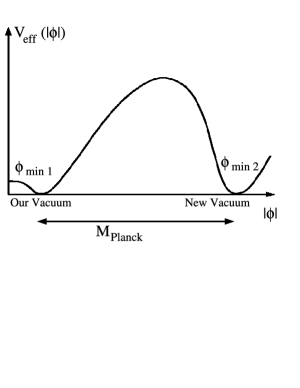
Figure 1: The first (our) vacuum at $|\phi|\approx 246$ GeV and the second vacuum at the fundamental scale $|\phi|\sim M_{Pl}$.

The model [6, 7, 8] in conjunction with MPP [10] fits well the SM fermion masses and mixing angles and describes all neutrino experimental data [14] (see below Section 7). This approach based on the FRGG-model was previously called Anti-Grand Unified Theory (AntiGUT).

In the present paper we discuss “AntiGUT” as a consequence of the existence of SUSY GUT $[E_{6}]^{3}$ near the Planck scale, which is predicted by our new preon model [15, 16, 17] producing three generations of composite quark-leptons and bosons. By this reason, we prefer not to use the name “AntiGUT” for the FRGG model (3) and call it simply “FNT-model” (Froggatt–Nielsen–Takanishi model [6, 7, 8, 14]).

1.2 Heterotic superstring theory $\boldsymbol{E_{8}\times E^{\prime}_{8}}$

Superstring theory gives the possibility to unify all fundamental gauge interactions with gravity. The authors of [18, 19, 20] have shown that superstrings are free of gravitational and Yang–Mills anomalies if the superstring theory is described by the gauge group of symmetry $SO(32)$ or $E_{8}\times E_{8}$. A more realistic candidate for unification is the “heterotic” superstring theory $E_{8}\times E^{\prime}_{8}$ suggested in [21, 22, 23]. This ten-dimensional Yang–Mills theory can undergo a compactification. The integration over six compactified dimensions leads to the effective theory with $E_{6}$ gauge group of symmetry in four dimensions. The group $E_{8}$ is broken, but $E^{\prime}_{8}$ remains unbroken and plays the role of a hidden sector in SUGRA. As a result, we obtain the $E_{6}$ SUSY-GUT in the four-dimensional space.

2 A new preon model of composite particles

In this paper, as in [15, 16, 17], we present a new model of preons making composite quark-leptons and (gauge and Higgs) bosons described by the three types of supersymmetric ‘flipped’ $E_{6}$ gauge groups of unification.

We start with the ‘flipped’ supersymmetric group $E_{6}\times\widetilde{E_{6}}$. Here $E_{6}$ is a non-dual sector of theory with the hyper-electric charge $g$, and $\widetilde{E_{6}}$ is a dual sector with the hyper-magnetic charge $\tilde{g}$.

2.1 Preons are dyons confined by hyper-magnetic strings

The main idea of our investigations, published in [15, 16, 17], is an assumption that preons are dyons confined by hyper-magnetic strings which are created by the condensation of spreons near the Planck scale.

J. Pati first suggested [24, 25] to use the strong $U(1)$ magnetic forces to bind preons-dyons in composite objects. This idea is extended in our model in the light of recent investigations of composite non-Abelian flux tubes in SQCD [26, 27, 28, 29, 30].

Considering the ${\rm\bf N}=1$ supersymmetric flipped $E_{6}\times\widetilde{E_{6}}$ gauge theory for preons in $4D$-dimensional space-time, we assume that preons $P$ and antipreons $P^{\rm\bf c}$ are dyons with charges ($ng$, $m\tilde{g}$) and ($-ng$, $-m\tilde{g}$), respectively, residing in the $4D$ hypermultiplets:

$${\cal H}=(P,P^{\rm\bf c})$$

and

$${\cal\tilde{H}}=(\tilde{P},{\tilde{P}}^{\rm\bf c}).$$

Here “$\tilde{P}$” designates spreons, but not the belonging to $\widetilde{E_{6}}$. We assume that the dual sector $\widetilde{E_{6}}$ is broken in our world for $\mu\leq{\tilde{\mu}}_{\rm crit}$ (where $\mu$ is the energy scale) to some group $\widetilde{G}$.

As a result, near the Planck scale preons and spreons transform under the hyper-electric gauge group $E_{6}$ and hyper-magnetic gauge group $\widetilde{G}$ according to their fundamental representations:

$$P,\tilde{P}\sim(27,N),\qquad P^{\rm\bf c},\tilde{P}^{\rm\bf c}\sim\left(\overline{27},\overline{N}\right),$$

where we consider the fundamental representation 27 for $E_{6}$ and $N$-plet for $\widetilde{G}$ group. We also take into account preons and spreons which are singlets of $E_{6}$:

$$P_{s},\tilde{P}_{s}\sim(1,N),\qquad P_{s}^{\rm\bf c},\tilde{P}_{s}^{\rm\bf c}\sim\left(1,\overline{N}\right).$$

They are actually necessary for the entire set of composite quark-leptons and bosons (see [31]).

The hyper-magnetic interaction is assumed to be responsible for the formation of $E_{6}$ fermions and bosons at the compositeness scale $\Lambda_{s}$.

2.2 String configurations of composite particles

Assuming that preons-dyons are confined by hyper-magnetic supersymmetric non-Abelian flux tubes which are a generalization of the well-known Abelian Abrikosov–Nielsen–Olesen (ANO) strings [32, 33], we have the following bound states in the limit of infinitely narrow flux tubes (strings):

• quark-leptons (fermions belonging to the $E_{6}$ fundamental representation):

  $$Q^{a}\sim P^{aA}(y)\left[{\cal P}\exp\left(i\tilde{g}\int_{x}^{y}\widetilde{A}_{\mu}dx^{\mu}\right)\right]_{A}^{B}{({\tilde{P}}_{s}^{\rm\bf c})}_{B}(x)\sim 27,$$

  where $a\in 27$-plet of $E_{6}$, $A,B\in N$-plet of $\widetilde{G}$, $\cal P$ is the path ordering and $\widetilde{A}_{\mu}(x)$ are dual vector potentials belonging to the adjoint representation of $\widetilde{G}$;

• “mesons” (hyper-gluons and hyper-Higgses of $E_{6}$):

  $$M^{a}_{b}\sim P^{aA}(y)\left[{\cal P}\exp\left(i\tilde{g}\int_{x}^{y}\widetilde{A}_{\mu}dx^{\mu}\right)\right]_{A}^{B}(P^{\rm\bf c})_{bB}(x)\sim 1+78+650\qquad{\rm of}\ E_{6},$$

  $$S\sim({\tilde{P}}_{s})^{A}(y)\left[{\cal P}\exp\left(i\tilde{g}\int_{x}^{y}\widetilde{A}_{\mu}dx^{\mu}\right)\right]_{A}^{B}{({\tilde{P}}_{s}^{\rm\bf c})}_{B}(x)\sim 1;$$

• for $\widetilde{G}$-triplet we have “diquarks”:

  $$D\sim\epsilon_{ABC}P^{aA^{\prime}}(z)P^{bB^{\prime}}(y)({\tilde{P}}_{s})^{C^{\prime}}(x)\left[{\cal P}\exp\left(i\tilde{g}\int^{z}_{X}\widetilde{A}_{\mu}dx^{\mu}\right)\right]_{A^{\prime}}^{A}$$

  $$\phantom{D\sim}{}\times\left[{\cal P}\exp\left(i\tilde{g}\int^{y}_{X}\widetilde{A}_{\mu}dx^{\mu}\right)\right]_{B^{\prime}}^{B}\left[{\cal P}\exp\left(i\tilde{g}\int^{x}_{X}\widetilde{A}_{\mu}dx^{\mu}\right)\right]_{C^{\prime}}^{C},$$

  and “baryons”:

  $$B\sim\epsilon_{ABC}P^{aA^{\prime}}(z)P^{bB^{\prime}}(y)P^{cC^{\prime}}(x)\left[{\cal P}\exp\left(i\tilde{g}\int^{z}_{X}\widetilde{A}_{\mu}dx^{\mu}\right)\right]_{A^{\prime}}^{A}$$

  $$\phantom{B\sim}{}\times\left[{\cal P}\exp\left(i\tilde{g}\int^{y}_{X}\widetilde{A}_{\mu}dx^{\mu}\right)\right]_{B^{\prime}}^{B}\left[{\cal P}\exp\left(i\tilde{g}\int^{x}_{X}\widetilde{A}_{\mu}dx^{\mu}\right)\right]_{C^{\prime}}^{C}.$$

The conjugate composite particles are constructed analogously.

The string configurations $D$ and $B$ describe a new type of composite particles belonging to the different representations of $E_{6}$.

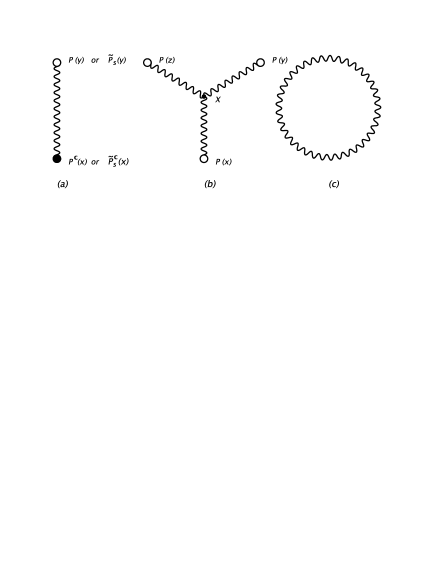
Figure 2: Preons are bound by hyper-magnetic strings: (a) corresponds to the “unclosed” string configurations of composite quark-leptons, hyper-gluons and hyper-Higgses; (b) corresponds to “baryonic” and “diquark” configurations; (c) represents a closed string describing a hyper-glueball (“graviton”).

The bound states are shown in Fig. 2. It is easy to generalize these string configurations for the case of superpartners – squark-sleptons, hyper-gluinos and hyper-higgsinos. All these bound states belong to $E_{6}$ representations and they in fact form ${\rm\bf N}=1$ $4D$ superfields.

3 Condensation of spreons near the Planck scale

Let us consider now the breakdown of $E_{6}$ and $\widetilde{E_{6}}$ groups at the Planck scale. We assume that Higgses belonging to the 78-dimensional representation of $E_{6}$ lead to the following breakdown:

$$E_{6}\to SU(6)\times SU(2)\to SU(6)\times U(1),$$

where $SU(6)\times U(1)$ is the largest relevant invariance group of the 78 [34]. Below we shall show that just this breakdown provides the spreon condensation and existence of the second vacuum.

In this investigation, in contrast to our previous papers [15, 16], we suggest to consider several types of possible chains for the SM extension by family replicated gauge groups leading to the $[E_{6}]^{3}$ unification near the scale $\sim 10^{17}$ GeV (according to the predictions of superstrings [18]). The chain (explained by the FNT-model [6, 7, 8, 14]):

$$SU(3)_{C}\times SU(2)_{L}\times U(1)_{Y}\to SU(3)_{C}\times SU(2)_{L}\times U(1)_{Z}\times U(1)_{X}$$

$$\qquad{}\to[SU(3)_{C}]^{3}\times[SU(2)_{L}]^{3}\times[U(1)_{Z}]^{3}\times[U(1)_{X}]^{3}$$ (4)

• can be extended by ‘flipped’ models [35]:

  $$\to[SU(5)\times U(1)_{X}]^{3}\to[SU(5)\times U(1)_{Z1}\times U(1)_{X1}]^{3}$$

  $$\qquad{}\to[SO(10)\times U(1)_{X1}]^{3}\to[E_{6}]^{3},$$ (5)

• or by three ways connected with the left-right symmetry [36, 37, 38]:

  $$\to[SU(4)_{C}]^{3}\times[SU(2)_{L}]^{3}\times[SU(2)_{R}]^{3}\times[U(1)_{Z}]^{3}$$

  $$\qquad{}\to[SO(10)\times U(1)_{Z}]^{3}\to[E_{6}]^{3},$$ (6)

  $$\to[SU(4)_{C}]^{3}\times[SU(2)_{L}]^{3}\times[SU(2)_{R}]^{3}\times[U(1)_{Z}]^{3}$$

  $$\qquad{}\to[SU(6)\times SU(2)_{R}]^{3}\to[E_{6}]^{3},$$ (7)

  $$\to[SU(3)_{C}]^{3}\times[SU(2)_{L}]^{3}\times[SU(2)_{R}]^{3}\times[U(1)_{X}]^{3}\times[U(1)_{Z}]^{3}$$

  $$\qquad{}\to[SU(3)_{C}]^{3}\times[SU(3)_{L}]^{3}\times[SU(3)_{R}]^{3}\to[E_{6}]^{3}.$$ (8)

In the present paper we have investigated only the case 1) of the ‘flipped’ models. We have chosen this case with the aim to obtain a minimum of the effective potential at the scale $\sim 10^{18}$ GeV (see below Section 6).

We have assumed as an Example 5 of [35] the breakdown of each supersymmetric ‘flipped’ $SU(5)\times U(1)_{X}$ to the non-supersymmetric gauge group $SU(3)_{C}\times SU(2)_{L}\times U(1)_{Z}\times U(1)_{X}$ at the scale $\sim 10^{15}$ GeV, using the condensates of the Higgs bosons belonging to the $5_{h}+\bar{5}_{h}$, $10_{H}+\overline{10}_{H}$, $15_{H^{\prime}}+\overline{15}_{H^{\prime}}$ and 24-dimensional adjoint A representations of the flipped $SU(5)$. Then the final unification group is the flipped $[E_{6}]^{3}$ at the scale $\sim 10^{17}$ GeV. It is obvious that in this case each $E_{6}$ is broken to $SO(10)\times U(1)_{X1}$ by condensates of the Higgs bosons belonging to the $27_{h}+\overline{27}_{h}$, $351_{H}+\overline{351}_{H}$, ${351^{\prime}}_{H^{\prime}}+\overline{351^{\prime}}_{H^{\prime}}$ and 78-dimensional adjoint A representations of the flipped $E_{6}$. In the intermediate region we have the condensates of the Higgs bosons belonging to the $10_{h}+\bar{1}0_{h}$, $45_{H}+\overline{45}_{H}$, $54_{H^{\prime}}+\overline{54}_{H^{\prime}}$ and 45-dimensional adjoint A representations of the flipped $SO(10)$.

Fig. 3 presents a qualitative description of the running of the inverse coupling constants $\alpha_{i}^{-1}(x)$ near the Planck scale predicted by the case 1) of our model in the one-loop approximation of the above-mentioned Example 5 of [35]. Here for $\alpha_{i}=g_{i}^{2}/4\pi$ index $i$ corresponds to the groups (4) and (5): $i=1,2,3,X,Z,X1,Z1,5,10$; $x=\log_{10}\mu$(GeV), and $\mu$ is the energy scale.

Of course, we must understand that the one-loop approximation running of $\alpha_{i}^{-1}(x)$ is not valid in the non-perturbative region $AB$. Two points $A$ and $B$, shown in Fig. 3, correspond (see [15, 16]): 1) to the scale $M_{\rm crit}$ of the breakdown $E_{6}\to SU(6)\times U(1)$ (point $A$), and 2) to the scale $\widetilde{M}_{\rm crit}$ of the breakdown $\widetilde{E_{6}}\to\widetilde{SU(6)}\times\widetilde{U(1)}$ (point $B$). We see that near the scale $M_{C}\approx 10^{18}$ GeV there exists just the theory of non-Abelian flux tubes, which was developed recently in [26, 27, 28, 29, 30]. In contrast to [15, 16, 17], it is necessary to choose $M_{C}<M_{Pl}$ with the aim not to come in conflict with gravity.

Figure 3: The figure provides a qualitative description of the running of $\alpha^{-1}(x)$ near the Planck scale predicted by the present preon model. The family replicated gauge group of symmetry $[E_{6}]^{3}$ exists in the region of energies $M_{SSG}\leq\mu\leq M_{\rm crit}$. The point $A$ at the scale of energy $\mu=M_{\rm crit}$ indicates that hyper-electric preon strings exist for $\mu\geq M_{\rm crit}$. The point $B$ corresponds to the scale $\mu=\widetilde{M}_{\rm crit}$ and indicates that hyper-magnetic preon strings exist for $\mu\leq\widetilde{M}_{\rm crit}$. The curve $AB$ corresponds to the region of spreon condensation, where we have both hyper-electric and hyper-magnetic strings. The point $C$ corresponds to the second vacuum of our theory. For $\mu\geq\widetilde{M}_{\rm crit}$ we have the running of $\alpha^{-1}(x)$ for monopolic “quark-leptons”, but gravity (SUGRA) transforms the trans-Planckian region. We assume that our theory is valid only up to the scale $\sim 10^{18}$ GeV (point $C$).

We assume the condensation of spreons near the scale $M_{C}$. One can combine the $Z_{6}$ center of $SU(6)$ with the elements $\exp(i\pi)\in U(1)$ to get topologically stable string solutions possessing both windings, in $SU(6)$ and $U(1)$. Henceforth, we assume the existence of a dual sector of the theory described by $\widetilde{SU(6)}\times\widetilde{U(1)}$, which is responsible for hyper-magnetic fluxes. Then we have a nontrivial homotopy group:

$$\pi_{1}\left(\frac{SU(6)\times U(1)}{Z_{6}}\right)=Z_{6},$$

and flux lines form topologically non-trivial $Z_{6}$ strings.

Besides $SU(6)$ and $U(1)$ gauge bosons, the model contains thirty six scalar fields charged with respect to $U(1)$ and $\widetilde{U(1)}$ which belong to the 6-plets of $SU(6)$ and $\widetilde{SU(6)}$. Considering scalar fields of spreons

$$\tilde{P}=\left\{\phi^{aA}\right\},\qquad a,A=1,2,\dots,6,$$

we construct their condensation in the vacuum:

$${\tilde{P}}_{\rm vac}=\big{\langle}\tilde{P}^{aA}\big{\rangle}=v\cdot{\rm diag}(1,1,\dots,1),\qquad a,A=1,\dots,6.$$

The vacuum expectation value (VEV) $v$ is given in [26] as

$$v=\sqrt{\xi}\gg\Lambda_{4},$$

where $\xi$ is the Fayet–Iliopoulos $D$-term parameter in the ${\rm\bf N}=1$ supersymmetric theory and $\Lambda_{4}$ is its 4-dimensional scale. In our case:

$$v\sim M_{C}\sim 10^{18}\,\,{\rm GeV},$$

because spreons are condensed near the scale $M_{C}$.

Non-trivial topology amounts to the winding of elements of the matrix

$$\tilde{P}=\left\{\phi^{aA}\right\},\qquad a,A=1,2,\dots,6,$$

and we obtain string solutions of the type:

$${\tilde{P}}_{\rm string}=v\cdot{\rm diag}\left(e^{i\alpha(x)},e^{i\alpha(x)},\dots,1,1\right),\qquad{\rm where}\,\quad x\to\infty.$$

Assuming the existence of a preon $P$ (or spreon $\tilde{P}$) and antipreon $P^{\rm\bf c}$ (antispreon $\tilde{P}^{\rm\bf c}$) at the ends of strings with hyper-magnetic charges $n\tilde{g}$ and $-n\tilde{g}$, respectively, we obtain the six types of strings having their fluxes $\Phi_{n}$ quantized according to the $Z_{6}$ center group of $SU(6)$ [21]:

$$\Phi_{n}=n\Phi_{0},\qquad n=\pm 1,\pm 2,\pm 3.$$

The string tensions of these non-Abelian flux tubes were also calculated. The minimal tension is:

$$T_{0}=2\pi\xi,$$

which in our preon model is equal to:

$$T_{0}=2\pi v^{2}\sim 10^{36}\,\,{\rm GeV}^{2}.$$

Such an enormously large tension means that preonic strings have almost infinitely small $\alpha^{\prime}\to 0$, where $\alpha^{\prime}=1/(2\pi T_{0})$ is the slope of trajectories in the string theory.

The six types of preonic flux tubes oriented in opposite directions give us the three types of preonic $k$-strings having the following tensions:

$$T_{k}=k\cdot T_{0},\qquad{\rm where}\quad k=1,2,3.$$

Then hyper-magnetic charges of preons (spreons) and antipreons (antispreons) are confined by three types of string.

Also preonic strings are extremely thin. It was shown in [15, 16] that the radius $R_{\rm str}$ of the flux tubes is very small: $R_{\rm str}\sim 10^{-18}\,\,{\rm GeV}^{-1}$.

4 Origin of three generations

We have obtained three, and only three, generations of fermions and bosons in the superstring-inspired ‘flipped’ $E_{6}$ model of preons. This number “3” is explained by the existence of just three values of hyper-magnetic flux tubes which bind the hyper-magnetic charges of preons-dyons. At the ends of the preonic strings there are placed hyper-magnetic charges:

$$\pm\tilde{g}_{0},\qquad{\rm or}\qquad\pm 2\tilde{g}_{0},\qquad{\rm or}\qquad\pm 3{\tilde{g}}_{0},$$

where ${\tilde{g}}_{0}$ is the minimal hyper-magnetic charge. Then all the bound states form three generations: for example, three 27-plets of $E_{6}$ corresponding to the three different tube fluxes. We have obtained a specific type of “horizontal symmetry” explaining flavor. It was shown in [15, 16] that the model explains the hierarchy of the SM masses naturally.

We also have obtained three types of gauge boson $A_{\mu}^{i}$ (where $i=1,2,3$ is the generation index) belonging to the $27\times\overline{27}=1+78+650$ representations of $E_{6}$.

Fig. 4 illustrates the formation of such hyper-gluons (Fig. 4(a)) and also hyper-Higgses (Fig. 4(b)).

Figure 4: Vector gauge bosons belonging to the 78 representation of the flipped $E_{6}$ and Higgs scalars – singlets of $E_{6}$ – are composite objects created (a) by fermionic preons $P$, $P^{\rm\bf c}$ and (b) by scalar spreons ${\tilde{P}}_{s}$, ${\tilde{P}}^{\rm\bf c}_{s}$. Both of them are confined by hyper-magnetic strings.

The existence of three generations of hyper-gluons predicts the family replicated $[E_{6}]^{3}$ unification near the scale $\sim 10^{17}$ GeV. Here the number of families is equal to the number of generations: $N_{\rm fam}=N_{\rm gen}=3$. The dynamical assumption of the three families in our preon model is based on the existence of the three types of flux tubes (“strings”) connecting preons-dyons in the three (and only three) types of hyper-gluons which create just the $[E_{6}]^{3}$ unification.

5 Family replicated $\boldsymbol{[E_{6}]^{3}}$ unification

The illustrative picture given in Fig. 3 presents the existence of $[E_{6}]^{3}$ unification in the region of energies $M_{SSG}\leq\mu\leq M_{\rm crit}$, where the unification scale $M_{SSG}\approx 10^{17}$ GeV.

Here it is necessary to distinguish $E_{6}$ gauge symmetry group for preons from $E_{6}$ for quark-leptons. The points $A$ and $B$ of Fig. 3 respectively correspond to the breakdown of $[E_{6}]^{3}$ and $[\widetilde{E_{6}}]^{3}$ in the region $AB$ of spreon condensation. In that region we have the breakdown of the preon (one family) $E_{6}$ (or $\widetilde{E_{6}}$):

$$E_{6}\to SU(6)\times U(1)\qquad\left({\rm or}\ \widetilde{E_{6}}\to\widetilde{SU(6)}\times\widetilde{U(1)}\right).$$

Fig. 3 shows that the group $E_{6}$ is broken in the region of energies $\mu\geq M_{\rm crit}$ producing hyper-electric strings between preons. The point $A$ ($B$) indicates the scale $M_{\rm crit}$ ($\widetilde{M}_{\rm crit}$) corresponding to the breakdown of $E_{6}$ ($\widetilde{E_{6}}$). At the point $B$ hyper-magnetic strings are produced and exist in the region of energies $\mu\leq\widetilde{M}_{\rm crit}$ confining hyper-magnetic charges of preons. As a result, in the region $\mu\leq M_{\rm crit}$ we see quark-leptons with hyper-electric charges, but in the region $\mu\geq\widetilde{M}_{\rm crit}$ monopolic “quark-leptons” – particles with hyper-magnetic charges – may exist. However, in this region which is close to $M_{Pl}$, our theory is not correct: gravity (SUGRA) begins to work, and monopoles are absent in our world.

The dotted curve in Fig. 3 describes the running of $\alpha^{-1}(\mu)$ for monopolic “quark-leptons” created by preons which are bound by supersymmetric hyper-electric non-Abelian flux tubes. The curve $AB$ corresponds to the region of spreon condensation, where we have both hyper-electric and hyper-magnetic strings. The point $C$ corresponds to the second vacuum of our theory. For $\mu\geq\widetilde{M}_{\rm crit}$ we have the running of monopole coupling constant. The corresponding $\alpha^{-1}(x)$ is shown in Fig. 3 by the dotted curve. But our theory is valid only up to the scale $\sim 10^{18}$ GeV (point $C$ of Fig. 3). Gravity (SUGRA) transforms the trans-Planckian region, and we do not know anything about the behavior of theory in the region of dotted curve.

5.1 The breakdown of $\boldsymbol{[E_{6}]^{3}}$ to the FNT-model

In general, it is quite possible to obtain the FNT-model considering the chain (4), (5) of the ‘flipped’ models at lower energies.

We may assume the breakdown of the supersymmetric ‘flipped’ $[SU(5)]^{3}$ to the non-supersymmetric FRGG:

$$[SU(3)_{C}]^{3}\times[SU(2)_{L}]^{3}\times[U(1)_{Z}]^{3}\times[U(1)_{X}]^{3}$$ (9)

at the scale $\sim 10^{15}$ GeV, what was shown in Fig. 3. Then the final unification group is the flipped $[E_{6}]^{3}$ at the scale $M_{SSG}\approx 10^{17}$ GeV.

With the aim to confirm the FNT-model scenario [6, 7, 8, 14], we must assume that the chain (5) from $[SU(5)]^{3}$ to $[E_{6}]^{3}$ is realized in the very narrow interval of energies. For example, in contrast to Fig. 3, we can consider the breakdown of the supersymmetric ‘flipped’ $[SU(5)]^{3}$ to the non-supersymmetric FRGG (9) at the scale $\sim 10^{17}$ GeV, assuming that $M_{SSG}\approx 10^{17.5}$ GeV. Shortly speaking, the group of unification $[E_{6}]^{3}$ undergoes an almost direct breakdown to the FRGG group (9).

As we have mentioned previously, the condensation of spreons near the scale $M_{C}$ predicts the existence of a second minimum of the effective potential at the scale $\mu\sim 10^{18}$ GeV (see Fig. 1), according to the Multiple Point Principle [10, 11, 12, 13].

6 Minimum of the effective potential near the Planck scale

It is not easy to guess how Nature can choose its path from the SM to the Planck scale. Different paths essentially depend on the fact whether the intermediate symmetry groups show asymptotically free or asymptotically unfree (or depressed) behavior of running gauge couplings. Such a behavior is connected with the number of representations of the Higgs bosons providing the breaking of the intermediate symmetry gauge groups down to the SM (what was considered in Section 3 for $SU(5)$ and $SO(10)$ groups of the chain (5)).

In our preon model the condensation of spreons is possible only if we have a minimum of the effective potential near the Planck scale. Not each of the paths (4)–(8) can give such a minimum. The paths (6)–(8) of the case 2) of Section 3 are presumably asymptotically free and do not give a minimum of the effective potential. As it was shown in [35], the $E_{6}$-unification can give such a minimum for the chain (4), (5) if there exist symmetry breaking Higgs bosons belonging to the representations given in Section 3 by the Example 5 of [35]. This is a simplest example, because more complicated cases can be considered.

In the non-Abelian theory, one usually starts with a gauge field $F_{\mu\nu}(x)$ derivable from a potential $A_{\mu}(x)$:

$$F_{\mu\nu}=\partial_{\nu}A_{\mu}(x)-\partial_{\mu}A_{\nu}(x)+ig[A_{\mu}(x),A_{\nu}(x)].$$

Considering only gauge groups with the Lie algebra of $SU(N)$, we have:

$$A_{\mu}(x)=t^{j}A_{\mu}^{j}(x),\qquad j=1,\dots,N^{2}-1,$$

where $t^{j}$ are the generators of $SU(N)$ group.

In general, the perturbative effective potential is given by the following expression (see [39, 40, 41, 42]):

$$V_{\rm ef\/f}^{(0)}=\frac{\alpha_{\rm ef\/f}^{-1}(F^{2})}{16\pi}F^{2}\qquad{\mbox{with}}\quad F^{2}\equiv F_{\mu\nu}^{j}F^{j\mu\nu}=(\mu\,\,{\mbox{GeV}})^{4}.$$ (10)

Here $\alpha_{\rm ef\/f}^{-1}(F^{2})=\alpha^{-1}(x)$ of our theory. However, the expression (10) is not valid in the non-perturbative region, because the non-perturbative vacuum contains a condensation of flux tubes (hyper-electric flux tubes in our theory of preons), according to the so called “spaghetti vacuum” by Nielsen–Olesen [43]. By this reason, we subtract the contribution of the condensed fluxes from the expression (10):

$$V_{\rm ef\/f}=\frac{\alpha_{\rm ef\/f}^{-1}(F^{2})-\alpha_{\rm ef\/f}^{-1}(F_{0}^{2})}{16\pi}F^{2},$$ (11)

where $F_{0}^{2}=(M_{C}\,\,{\mbox{GeV}})^{4}$. From (11) we have:

$$V_{\rm ef\/f}(x)=\frac{\alpha^{-1}(x)-\alpha^{-1}(x_{c})}{16\pi}10^{4x}.$$

The behavior of the effective potential $V_{\rm ef\/f}(x)$ is given in Fig. 5, where we see a second minimum near the Planck scale at the point $\mu=M_{C}=10^{18}$ GeV. For this minimum we have:

$$V_{\rm ef\/f}=V^{\prime}_{\rm ef\/f}=0,$$

according to the MPP [10, 11, 12, 13]. But at the scale $M_{C}$ our theory stops (it is not valid), and we do not know the development of our theory up to the Planck scale and further – in trans-Planckian region.

Figure 5: The behavior of the effective potential $V_{\rm ef\/f}(x)$ for the $E_{6}^{3}$ theory, showing a second minimum of our theory at the point $\mu=M_{C}=10^{18}$ GeV. This minimum is given by the requirement: $V_{\rm ef\/f}=V^{\prime}_{\rm ef\/f}=0$, according to the Multiple Point Principle.

7 FNT-model, its advantages and shortcomings

If one extends the SM with the FNT-model (3) (or with any FRGG-model) not considering its GUT’s origin, then the theory has some problems. Such a theory

• would not account for the quantization of electric (or magnetic) charge, or for any quantum numbers of the members in a family, without additional assumptions;

• cannot give a prediction for the weak angle;

• cannot automatically possess B–L as a local symmetry and the righthanded neutrinos: they are put in by hand.

But SUSY GUTs solve these problems in a compelling manner. GUTs have a predictive power concerning the representations occurring in the SM. By this reason, it is useful to start with a SUSY GUT theory explaining the origin of the one or another FRGG-model if we have indications that this model is valid. SUSY GUT $[E_{6}]^{3}$ predicted by our preon model can be an explanation of the FNT-model.

However, in a slightly broader way we could think about comparing of the two competing types of models and see how well they fit and explain the putting of representations for the matter fields. Such an investigation was published for the FNT-model in [6, 7, 8, 9, 14]. It was shown that 6 different Higgs fields: $\omega$, $\rho$, $W$, $T$, $\phi_{WS}$, $\phi_{B-L}$ break the FNT-model to the SM. The field $\phi_{WS}$ corresponds to the Weinberg–Salam Higgs field of Electroweak theory. Its vacuum expectation value (VEV) is fixed by the Fermi constant: $\left\langle\phi_{WS}\right\rangle=246$ GeV, so that we have only 5 free parameters – five VEVs: $\left\langle\omega\right\rangle$, $\left\langle\rho\right\rangle$, $\left\langle W\right\rangle$, $\left\langle T\right\rangle$, $\left\langle\phi_{B-L}\right\rangle$ to fit the experiment in the framework of the SM. These five adjustable parameters were used with the aim of finding the best fit to experimental data for all fermion masses and mixing angles in the SM, and also to explain the neutrino oscillation experiments. It is assumed that the fundamental Yukawa couplings in our model are of order unity and so we make order of magnitude predictions.

Experimental results on solar neutrino and atmospheric neutrino oscillations from Sudbury Neutrino Observatory (SNO Collaboration) and the Super-Kamiokande Collaboration have been used to extract the following parameters:

$$\Delta m^{2}_{\rm solar}=m_{2}^{2}-m_{1}^{2},\qquad\Delta m^{2}_{\rm atm}=m_{3}^{2}-m_{2}^{2},$$

$$\tan^{2}\theta_{\rm solar}=\tan^{2}\theta_{12},\qquad\tan^{2}\theta_{\rm atm}=\tan^{2}\theta_{23}$$

where $m_{1}$, $m_{2}$, $m_{3}$ are the hierarchical left-handed neutrino effective masses for the three families.

The typical fit for the FNT-model is shown in Table 1. As we can see, the 5 parameter order of magnitude fit is encouraging.

Table 1: Best fit to conventional experimental data. All masses are running masses at $1~{}\mbox{\rm GeV}$ except the top quark mass which is the pole mass.

	Fitted	Experimental
$m_{u}$	4.4 MeV	4 MeV
$m_{d}$	4.3 MeV	9 MeV
$m_{e}$	1.6 MeV	0.5 MeV
$m_{c}$	0.64 GeV	1.4 GeV
$m_{s}$	295 MeV	200 MeV
$m_{\mu}$	111 MeV	105 MeV
$M_{t}$	202 GeV	180 GeV
$m_{b}$	5.7 GeV	6.3 GeV
$m_{\tau}$	1.46 GeV	1.78 GeV
$V_{us}$	0.11	0.22
$V_{cb}$	0.026	0.041
$V_{ub}$	0.0027	0.0035
$\Delta m^{2}_{\odot}$	$9.0\times 10^{-5}~{}\mbox{\rm eV}^{2}$	$5.0\times 10^{-5}~{}\mbox{\rm eV}^{2}$ 0.5ex
$\Delta m^{2}_{\rm atm}$	$1.7\times 10^{-3}~{}\mbox{\rm eV}^{2}$	$2.5\times 10^{-3}~{}\mbox{\rm eV}^{2}$ 0.5ex
$\tan^{2}\theta_{\odot}$	0.26	0.340.5ex
$\tan^{2}\theta_{\rm atm}$	0.65	1.00.5ex
$\tan^{2}\theta_{\rm chooz}$	2.9 $\times 10^{-2}$	$<2.6\times 10^{-2}$ 0.5ex

Here attention may drawn to the fact that for quite a long time now BNP-model (2) by Bennett–Nielsen–Picek [3] and FNT-model have been to assume that any physics beyond the SM will first appear at roughly the Planck scale (see [3, 4, 5, 10, 13, 14, 44, 45]). A justification for continuing to use this so-called “desert scenario” could be to demonstrate that the effects of the U(1)_(B-L) gauge group associated with the appearance of heavy right-handed neutrinos at $\sim$ 10¹⁵ GeV can be neglected for our study of the values of the fine structure constants near the Planck scale.

Assuming such a desert, in earlier works invented the MPP/AntiGUT gauge group model [3, 4, 10] for the purpose of predicting the Planck scale values of the three Standard Model Group (SMG) gauge couplings [3, 4, 5, 10, 13, 14, 44, 45], these predictions were made independently for the three gauge couplings of $SU(3)$, $SU(2)$ and $U(1)$ gauge theories.

According to the BNP-model (2), the fundamental group $SMG^{3}$ undergoes spontaneous breakdown to the diagonal subgroup at the energy scale $\mu=\mu_{G}\sim 10^{17}$ GeV:

$$SMG^{3}\to SMG^{3}_{\rm diag}=\{g,g,g|g\in SMG\}\cong SMG.$$

For this diagonal subgroup ${(SMG)^{3}}_{\rm diag}$, which is identified with the usual SMG, the gauge couplings are predicted to coincide with the experimental gauge group couplings at the Planck scale which in turn are related with critical (i.e., multiple point) couplings for $SMG^{3}$ [10] as follows (see also [44, 45]):

$$\alpha_{1,\exp}^{-1}(\mu_{Pl})=6\alpha_{1,{\rm crit}}^{-1},\qquad\alpha_{2,\exp}^{-1}(\mu_{Pl})=3\alpha_{2,{\rm crit}}^{-1},\qquad\alpha_{3,\exp}^{-1}(\mu_{Pl})=3\alpha_{3,{\rm crit}}^{-1}.$$

Here $\alpha_{i}(\mu)$ (where the indices $i=1,2,3$ correspond in same order to $U(1)$, $SU(2)$ and $SU(3)$ gauge groups of the SM) are the SM fine structure constants. Using renormalization group equations (RGEs) with parameters experimentally established at the Electroweak (EW) scale, it is possible to extrapolate the experimental values of the three inverse running constants $\alpha_{i}^{-1}(\mu)$ from EW scale to the Planck scale. The precision of the LEP data allows us to make this extrapolation with small errors [46] even when we ignore the appearance of the $U(1)_{(B-L)}$ group at the $\mu_{\rm seesaw}\sim 10^{15}$ GeV. Doing the RG extrapolation of the $\alpha^{-1}_{i}(\mu)$ with one Higgs doublet and using the assumption of no relevant new physics up to $\mu\approx\mu_{Pl}$ lead to the following values (see the Particle Data Group results [46]):

$$\alpha_{1,\exp}^{-1}(\mu_{Pl})\approx 55.4\pm 6,\qquad\alpha_{2,\exp}^{-1}(\mu_{Pl})\approx 49.0\pm 3,\qquad\alpha_{3,\exp}^{-1}(\mu_{Pl})\approx 53.0\pm 3.$$ (12)

In [3, 4, 5, 10, 13, 14, 44, 45] BNP-model gives an explanation of these values of the SM coupling constants existing near the Planck scale.

Also it is necessary to emphasize that FRGG models are extremely useful for the existence of monopoles in our Universe. Values (12) mean that monopoles are absent in the SM: they have a huge magnetic charge and are completely confined or screened. Supersymmetry does not help to see monopoles.

In theories with the FRGG-symmetry the charge of monopoles $\tilde{g}_{i}$ ($\tilde{\alpha}=\tilde{g}^{2}/{4\pi}$) is essentially diminished. FRGGs of type $[SU(N)]^{N_{\rm fam}}$ lead to the lowering of the magnetic charge of the monopole belonging to one family:

$$\tilde{\alpha}_{\rm one\,\,family}=\frac{\tilde{\alpha}}{N_{\rm fam}}.$$

For $N_{\rm fam}=3$, for $[SU(2)]^{3}$ and $[SU(3)]^{3}$, we have:

$$\tilde{\alpha}_{\rm one\,\,family}^{(2,3)}=\frac{{\tilde{\alpha}}^{(2,3)}}{3}.$$

For the family replicated group $[U(1)]^{N_{\rm fam}}$ we obtain:

$$\tilde{\alpha}_{\rm one\,\,family}=\frac{\tilde{\alpha}}{N^{*}}$$

where $N^{*}=\frac{1}{2}N_{\rm fam}(N_{\rm fam}+1)$. For $N_{\rm fam}=3$ and $[U(1)]^{3}$, we have: $\tilde{\alpha}_{\rm one\,\,family}^{(1)}={\tilde{\alpha}}^{(1)}/6$ (six times smaller!). This result was obtained previously in [10, 47, 48]. We conclude: FRGG models help to observe monopoles in Nature.

Recent investigations [44, 45] are devoted to the Planck scale values of monopole coupling constants. With help of MPP and FRGG-models we discover new possibilities for monopoles, for dual charges in general.

8 Conclusions and discussions

In the present paper we have developed a new model of preons suggested in [15, 16, 17]. According to this model, preons construct composite quark-leptons and (gauge and Higgs) bosons which are described by the three types of supersymmetric ‘flipped’ $E_{6}$ gauge groups of unification. Crucial points of this model are: 1) the $E_{6}$-unification for preons inspired by Superstring theory [18, 19, 20, 21, 22, 23], and 2) the dynamical assumption that preons are dyons confined by supersymmetric non-Abelian hyper-magnetic flux tubes of type suggested in [26, 27, 28, 29, 30].

The $E_{6}$ gauge group of symmetry can be broken into $SU(6)\times U(2)$ – from one side, and into $SO(10)\times U(1)$ – from the second side. We have assumed that near the Planck scale Higgses belonging to the 78-dimensional representation of $E_{6}$ gave the breakdown $E_{6}\to SU(6)\times SU(2)\to SU(6)\times U(1)$, where $SU(6)\times U(1)$ is the largest relevant invariance group of the 78 [34]. Assuming the condensation of spreons near the Planck scale, we have combined the $Z_{6}$ center of $SU(6)$ with the elements $\exp(i\pi)\in U(1)$ to get topologically stable string solutions possessing both windings, in $SU(6)$ and $U(1)$. Just this $Z_{6}$ center of $SU(6)$ explains the existence of the three types of preonic $k$-strings associated with the three generations of quarks-leptons and bosons. Thus, in our preon model the dynamical properties of preons-dyons predict the three (and only three) generations (families) of composite quarks-leptons and bosons. In particular, such a dynamical picture leads to the existence of the three types of gauge bosons $A_{\mu}^{i}$ (where $i=1,2,3$ is the generation index) belonging to the $27\times\overline{27}=1+78+650$ representations of $E_{6}$. These three generations of hyper-gluons predict the family replicated unification $[E_{6}]^{3}=E_{6}\times E_{6}\times E_{6}$ near the scale $\sim 10^{17}$ GeV.

In the present paper we have considered the possibility of the further breakdown of the SUSY GUT $[E_{6}]^{3}$ into the Froggatt–Nielsen–Takanishi (FNT) model $[SU(3)_{C}]^{3}\times[SU(2)_{L}]^{3}\times[U(1)_{Y}]^{3}\times[U(1)_{(B-L)}]^{3}$ [6, 7, 8, 14], existing at lower energies. We have discussed in Section 7 all shortcomings and advantages of this model. Among its shortcomings we have no possibility to predict $U(1)_{B-L}$ gauge group of symmetry and seesaw scale.

We have presented the following advantages of the FNT-model: the possibility to fit the SM parameters (masses and mixing angles), the description of the Planck scale values of the three SM gauge couplings, the prediction of the Planck scale values of monopole couplings etc.

In Section 6 we have presented investigation of the existence of the second minimum of the effective potential in our preon model, in accordance with the Multiple Point Principle suggested in [10, 11, 12, 13].

Acknowledgments

The authors deeply thank Professor H.B. Nielsen and one of the anonymous referees for useful discussions and advices. We are thankful of the Organizing Committee of the Seventh International Conference ‘Symmetry in Nonlinear Mathematical Physics’ (Symmetry–2007) (June 24–30, 2007, Kyiv, Ukraine) where our talk was presented.

This work was supported by the Russian Foundation for Basic Research (RFBR), project No 05–02–17642.

References

- [1]
- [2] Wilczek F., Zee A., Horizontal interaction and weak mixing angles, Phys. Rev. Lett. 42 (1979), 421–425.
- [3] Bennett D.L., Nielsen H.B., Picek I., Understanding fine structure constants and three generations, Phys. Lett. B 208 (1988), 275–280.
- [4] Froggatt C.D., Nielsen H.B., Origin of symmetries, Singapore, World Scientific, 1991.
- [5] Laperashvili L.V., The standard model and the fine structure constant at Planck distances in Bennet–Brene–Nielsen–Picek random dynamics, Yad. Fiz. 57 (1994), 501–508 (English transl.: Phys. Atom. Nucl. 57 (1994), 471–478).
- [6] Nielsen H.B., Takanishi Y., Neutrino mass matrix in anti-GUT with seesaw mechanism, Nuclear Phys. B 604 (2001), 405–425, hep-ph/0011062.
- [7] Nielsen H.B., Takanishi Y., Baryogenesis via lepton number violation in anti-GUT model, Phys. Lett. B 507 (2001), 241–251, hep-ph/0101307.
- [8] Froggatt C.D., Nielsen H.B., Takanishi Y., Family replicated gauge groups and large mixing angle solar neutrino solution, Nuclaer Phys. B 631 (2002), 285–306, hep-ph/0201152.
- [9] Froggatt C.D., Laperashvili L.V., Nielsen H.B., Takanishi Y., Family replicated gauge group models, in Proceedings of Fifth International Conference “Symmetry in Nonlinear Mathematical Physics” (June 23–29, 2003, Kyiv), Editors A.G. Nikitin, V.M. Boyko, R.O. Popovych and I.A. Yehorchenko, Proceedings of Institute of Mathematics, Kyiv 50 (2004), Part 2, 737–743, hep-ph/0309129.
- [10] Bennett D.L., Nielsen H.B., Prediction for nonabelian fine structure constants from multicriticality, Internat. J. Modern Phys. A 9 (1994), 5155–5200, hep-ph/9311321.
- [11] Froggatt C.D., Nielsen H.B., Standard model criticality prediction: top mass GeV and Higgs mass GeV, Phys. Lett. B 368 (1996), 96–102, hep-ph/9511371.
- [12] Froggatt C.D., Laperashvili L.V., Nielsen H.B., The fundamental-weak scale hierarchy in the standard model, Phys. Atom. Nucl. 69 (2006), 67–80, hep-ph/0407102.
- [13] Das C.R., Laperashvili L.V., Phase transition in gauge theories, monopoles and the multiple point principle, Internat. J. Modern Phys. A 20 (2005), 5911–5988, hep-ph/0503138.
- [14] Froggatt C.D., Nielsen H.B., Trying to understand the standard model parameters, Invited talk by H.B. Nielsen at the “XXXI ITEP Winter School of Physics” (February 18–26, 2003, Moscow, Russia), Surveys High Energy Phys. 18 (2003), 55–75, hep-ph/0308144.
- [15] Das C.R., Laperashvili L.V., Are preons dyons? Naturalness of three generations, Phys. Rev. D 74 (2006), 035007, 12 pages, hep-ph/0605161.
- [16] Das C.R., Laperashvili L.V., Composite model of quark-leptons and duality, hep-ph/0606042.
- [17] Laperashvili L.V., Das C.R., Dyons near the Planck scale, Internat. J. Modern Phys. A 22 (2007), 5211–5228, hep-ph/0606043.
- [18] Green M.B., Schwarz J.H., Witten E., Superstring theory, Vol. 1, 2, Cambridge University Press, Cambridge, 1988.
- [19] Green M.B., Schwarz J.H., Anomaly cancellation in supersymmetric gauge theory and superstring theory, Phys. Lett. B 149 (1984), 117–122.
- [20] Green M.B., Schwarz J.H., Infinity cancellations in superstring theory, Phys. Lett. B 151 (1985), 21–25.
- [21] Gross D.J., Harvey J.A., Martinec E., Rohm R., The heterotic string, Phys. Rev. Lett. 54 (1985), 502–505.
- [22] Gross D.J., Harvey J.A., Martinec E., Rohm R., Heterotic string theory. 1. The free heterotic string, Nuclear Phys. B 256 (1985), 253–284.
- [23] Gross D.J., Harvey J.A., Martinec E., Rohm R., Heterotic string theory. 2. The interacting heterotic string, Nuclear Phys. B 267 (1986), 75–124.
- [24] Pati J.C., Magnetism as the origin of preon binding, Phys. Lett. B 98 (1981), 40–44.
- [25] Pati J.C., Salam A., Strathdee J., A preon model with hidden electric and magnetic type charges, Nuclear Phys. B 185 (1981), 416–428.
- [26] Marshakov A., Yung A., Non-Abelian confinement via Abelian flux tubes in softly broken SUSY QCD, Nuclear Phys. B 647 (2002), 3–48, hep-th/0202172.
- [27] Markov V., Marshakov A., Yung A., Non-Abelian vortices in gauge theory, Nucl. Phys. B 709 (2005), 267–295, hep-th/0408235.
- [28] Gorsky A., Shifman M.,Yung A., Non-Abelian Meissner effect in Yang–Mills theories at weak coupling, Phys. Rev. D 71 (2005), 045010, 16 pages, hep-th/0412082.
- [29] Shifman M., Yung A., Non-Abelian flux tubes in SQCD: supersizing world-sheet supersymmetry, Phys. Rev. D 72 (2005), 085017, 19 pages, hep-th/0501211.
- [30] Auzzi R., Shifman M., Yung A., Composite non-Abelian flux tubes in SQCD, Phys. Rev. D 73 (2006), 105012, 15 pages, Erratum, Phys. Rev. D 76 (2007), 109901, 3 pages, hep-th/0511150.
- [31] Chaichian M., Chkareuli J.L., Kobakhidze A., Composite quarks and leptons in higher space-time dimensions, Phys. Rev. D 66 (2002), 095013, 7 pages, hep-ph/0108131.
- [32] Abrikosov A.A., On the magnetic properties of superconductors of the second group, Zh. Eksp. Teor. Fiz. 32 (1957), 1442–1452 (English transl.: Sov. Phys. JETP 5 (1957), 1174–1182).
- [33] Nielsen H.B., Olesen P., Vortex line models for dual strings, Nuclear Phys. B 61 (1973), 45–61.
- [34] Cecotti S., Derendinger J.P., Ferrara S., Girardello L., Properties of breaking and superstring theory, Phys. Lett. B 156 (1985), 318–326.
- [35] Das C.R., Laperashvili L.V., Seesaw scales and the steps from the standard model towards superstring-inspired flipped , hep-ph/0604052.
- [36] Pati J.C., Salam A., Lepton number as the fourth color, Phys. Rev. D 10 (1974), 275–289, Erratum, Phys. Rev. D 11 (1975), 703–703.
- [37] Mohapatra R.N., Pati J.C., Left-right gauge symmetry and an isoconjugate model of CP violation, Phys. Rev. D 11 (1975), 566–571.
- [38] Mohapatra R.N., Pati J.C., A natural left-right symmetry, Phys. Rev. D 11 (1975), 2558–2561.
- [39] Kovalenko P.A., Laperashvili L.V., The effective QCD Lagrangian and renormalization group approach, Yad. Fiz. 62 (1999), 1857–1867 (English transl.: Phys. Atom. Nucl. 62 (1999), 1729–1738), hep-ph/9711390.
- [40] Matinyan S.G., Savvidy G.K., Vacuum polarization induced by the intense gauge field, Nuclear Phys. B 134 (1978), 539–545.
- [41] Matinyan S.G., Savvidy G.K., On the radiative corrections to classical Lagrangian and dynamical symmetry breaking, Yad. Fiz. 25 (1977), 218–226.
- [42] Batalin I.A., Matinyan S.G., Savvidy G.K., Vacuum polarization by a source-free gauge field, Yad. Fiz. 26 (1977), 407–414 (English transl.: Sov. J. Nucl. Phys. 26 (1977), 214–217).
- [43] Nielsen H.B., Olesen P., A quantum liquid model for the QCD vacuum gauge and rotational invariance of domained and quantized homogeneous color fields, Nuclear Phys. B 160 (1979), 380–396.
- [44] Bennett D.L., Laperashvili L.V., Nielsen H.B., Relation between finestructure constants at the Planck scale from multiple point principle, in Proceedings of the 9th Workshop on “What Comes Beyond the Standard Model” (September 16–26, 2006, Bled, Slovenia), Editors S. Ansoldi et al., DMFA-Zaloznistvo, Ljubljana, Slovenia (2006), 10–24, hep-ph/0612250.
- [45] Bennett D.L., Laperashvili L.V., Nielsen H.B., Finestructure constants at the Planck scale from multiple point principle, in Proceedings of the 10th Workshop on “What Comes Beyond the Standard Model” (July 17–27, 2007, Bled, Slovenia), Editors N. Mankoc Borstnik et al., DMFA-Zaloznistvo, Ljubljana, Slovenia 8 (2007), no. 2, 1–30, arXiv:0711.4681.
- [46] Yao W.-M. et al. (Particle Data Group), Review of particle physics, J. Phys. G 33 (2006), 1–1232.
- [47] Laperashvili L.V., Nielsen H.B., The problem of monopoles in the standard and family replicated models, in Proceedings of the 11th “Lomonosov Conference on Elementary Particle Physics” (August 21–27, 2003, Moscow, Russia), “Moscow 2003, Particle Physics in Laboratory, Space and Universe”, 2003, 331–337, hep-th/0311261.
- [48] Laperashvili L.V., Nielsen H.B., Ryzhikh D.A., Monopoles and family replicated unification, Yad. Fiz. 66 (2003), 2119–2127 (English transl.: Phys. Atom. Nucl. 66 (2003), 2070–2077), hep-th/0212213.