Bulk-edge coupling in the non-abelian $\nu=5/2$ quantum Hall interferometer

Abstract

Recent schemes for experimentally probing non-abelian statistics in the quantum Hall effect are based on geometries where current-carrying quasiparticles flow along edges that encircle bulk quasiparticles, which are localized. Here we consider one such scheme, the Fabry-Perot interferometer, and analyze how its interference patterns are affected by a coupling that allows tunneling of neutral Majorana fermions between the bulk and edge. While at weak coupling this tunneling degrades the interference signal, we find that at strong coupling, the bulk quasiparticle becomes essentially absorbed by the edge and the intereference signal is fully restored.

Recently, interference experiments were proposed as a way to examine the non-abelian nature of quasiparticles in the $\nu=5/2$ quantum Hall statereview ; stern06 ; bonderson06 ; dassarma05 . The most dramatic signature of non-abelian statistics is expected to be seen in the interference of back-scattering amplitudes from two constrictions in a long Hall bar. (See inset in Fig. 1.) The two constrictions enclose a “cell”, whose area may be varied by means of a side-gate. The bulk is assumed to host a number $N_{qp}$ of localized quasiparticles, that do not take part in electronic transport, and have no tunnel coupling to the edge. In the limit of weak back-scattering, when $N_{qp}$ is even the two back-scattering amplitudes interfere coherently, while when $N_{qp}$ is odd they are incoherent, and thus do not interfere. In the former case, the back-scattered current oscillates with the area of the cell, while in the latter case it does not. This difference reflects the non-abelian nature of the quasiparticles.

The theoretical analysis makes a sharp distinction between bulk and edge. In a real system, however, some degree of coupling between the edge and quasiparticles localized in the bulk is unavoidable. Since both the $5/2$ edge and the quasiparticles consist of both neutral Majorana fermionic and charged bosonic degrees of freedom, several types of edge to bulk coupling are possible. We expect that at low energies, tunneling that involves a charge will generally be suppressed due to the Coulomb energy. Thus in this work we will focus on tunneling of the neutral Majorana mode from the bulk to the edge, and on the resulting effect on the interference.

The system we consider chamon97 ; fradkin98 ; stern06 ; bonderson06 is a Hall bar lying parallel to the $x$–axis (See Fig. 1). Two constrictions are located at $x=-b$ and $x=b$. We focus on a simple case where there are two quasiparticles, $N_{qp}=2$, localized at $x=0$, between the two constrictions, with one of the quasiparticles coupled to the upper edge and the other coupled to the lower edge. Ref. Wen considers the case of $N_{qp}=1$ in the weak tunneling limit.

When the two localized quasiparticles are decoupled from the edge they form a two level system, and the ground state is doubly degenerate. The interference patterns that are seen in the two respective ground states are mutually shifted by a phase $\pi$. Then, at temperature $T=0$ the magnitude of the interference term depends on the ratio of two time scales, one determined by the voltage $t_{V}=\hbar/e^{*}V$, and the other being the time associated with motion between the two constrictions $t_{b}=2b/v$ where $v$ is a characteristic edge mode velocity. When analyzing the effect of bulk-edge coupling we will focus on the case of low voltage, $t_{V}\gg t_{b}$, where the interference is most clearly seen.

We start with a qualitative description of our results. In the absence of edge-bulk coupling the system cannot switch from one ground state to another. Thus if it is prepared in one ground state, repetitive measurements of the interference would show the same interference pattern. However, when the interference term is averaged over the two possible ground states, e.g., by measuring the interference with a random choice of the initial ground state, the average is zero. When the coupling of the bulk two-level system to the edge is turned on, the average value of the interference term becomes non-zero, and the correlation function between consecutive measurements is strongly modified. Denoting the coupling strengths between the localized Majorana particles and their respective edges by $\lambda_{u}$ and $\lambda_{d}$, [defined precisely in Eq. (1) below], we obtain corresponding time scales $t_{\lambda u(d)}=(\pi\lambda^{2}_{u(d)}/2v_{m})^{-1}$, where $v_{m}$ is the velocity of the Majorana modes on the edges. In the limit of weak coupling, where $t_{\lambda u(d)}\gg t_{V}$, we may use a perturbation analysis, and we find that the average value of the interference is proportional to $(t_{V})^{1/2}(t_{V}/t_{\lambda})\log^{2}[t_{\lambda}/t_{V}]$, where we have assumed that $t_{\lambda u}$ and $t_{\lambda d}$ are comparable in magnitude, and $t_{\lambda}$ is their geometric mean. As the coupling is increased, or as the voltage is lowered, the perturbative analysis breaks down. We then carry out a numerical analysis, which suggests that in the limit $t_{V}/t_{\lambda}\rightarrow\infty$ the full magnitude of the interference term is retrieved. In effect, the two bulk quasiparticles become then a part of the edge, and $N_{qp}$ reduces from two to zero. (We find a similar effect for a single quasiparticle strongly coupled to an edge.) In contrast to the build-up of the average interference term as the coupling gets stronger, the fluctuating part of the interference pattern is weakened by the coupling, and its characteristic correlation time becomes $t_{\lambda}$, which decreases with increased coupling.

For the derivation of these results we will follow several steps. After the introduction of the relevant Lagrangians, we derive the operator that describes quasiparticle tunneling across the two constrictions in the presence of the two localized bulk quasiparticles. We find it useful to represent this operator in two forms, a local form using the $\sigma$ operator of the Ising Conformal Field Theory (CFT) that describes the $\nu=5/2$ edge, and a non-local form in terms of the Majorana fermions that propagate along the edge. Within the non-local form, we show that the tunneling operator is proportional to a “parity operator” that measures the parity of the number of electrons encircled by a back-scattered quasiparticle as it moves from $x=-\infty$ along one edge, through the back-scattering at the constriction, back to $x=-\infty$ along the other edge. Next, we perturbatively analyze the weak coupling limit, and finally we numerically analyze the strong coupling limit.

In the absence of any coupling to bulk quasiparticles the upper ($u$) and lower ($d$) edges of the $\nu=5/2$ state are described by two charged boson fields $\phi_{u}(x),\phi_{d}(x)$ and a neutral Majorana fermion field. The Lagrangian for the boson field on each edge is that of a chiral Luttinger liquid, characterized by a velocity $\pm v_{c}$. The Lagrangian density for the Majorana fermion field is ${\cal L}_{m}^{r}={1\over 4\pi}\psi^{r}(x)[\partial_{t}-v_{m}^{r}\partial_{x}]\psi^{r}(x)$ with $r$ taking the values $u$ and $d$ for the upper and lower edges. For simplicity we set the velocities of the Majorana edge modes to be equal and opposite $v_{m}^{u}=-v_{m}^{d}=v_{m}$. Furthermore, we set $v_{m}=1$ when no confusion results. The Majorana Lagrangian can also be thought of as the Lagrangian of an Ising CFT YellowBook .

Each of the two localized bulk quasiparticles carries a zero mode, described by a localized Majorana operator. We denote the two bulk Majorana operators by $\gamma_{u},\gamma_{d}$, with the subscript indicating the edge to which the quasiparticle couples. The two-dimensional Hilbert space created by the two Majorana modes is spanned by the two eigenvectors of the operator $i\gamma_{u}\gamma_{d}$.

To examine the effects of bulk-edge coupling we couple $\gamma_{u}$ to the upper edge and $\gamma_{d}$ to the lower edge, both at $x=0$. The Lagrangian density for this coupling is

$${\cal L}_{b-e}=i\left[\lambda_{u}\psi^{u}(x)\gamma_{u}+\lambda_{d}\psi^{d}(x)\gamma_{d}\right]\delta(x)\ \ .$$ (1)

The Lagrangian ${\cal L}_{m}^{u}+{\cal L}_{m}^{d}+{\cal L}_{b-e}$ introduces the time scales $t_{\lambda u(d)}$ defined above. The bulk-edge coupling mixes the states with eigenvalues $\pm 1$ of $i\gamma_{u}\gamma_{d}$. Roughly speaking, $t_{\lambda}$ is the time in which a state with a particular value of $i\gamma_{u}\gamma_{d}$ decays to a mixture of the two eigenvalues.

The operator that tunnels a quasiparticle across a constriction may be expressed in a local form through the $\sigma_{u},\sigma_{d}$ operators of the Ising CFT that describes the $\nu=5/2$ upper and lower edges SBPRB . The tunnelling operator is $H_{tun}\equiv{\hat{T}}+{\hat{T}}^{+}$, where

$${\hat{T}}=e^{ie^{*}Vt}\left[\eta_{L}{\cal C}_{L}{\cal N}_{L}+\eta_{R}{\cal C}_{R}{\cal N}_{R}i\gamma_{u}\gamma_{d}\right]$$ (2)

transfers a quasiparticle from the lower to the upper edge through the left $(L)$ and right $(R)$ constrictions respectively, and its hermitian conjugate ${\hat{T}}^{+}$ similarly transfers a quasiparticle from the upper to the lower edge. Here, $V$ is the voltage difference between the two edges, $e^{*}=e/4$ is the quaisparticle charge. Correspondingly, the current operator is given by $J=\frac{e^{*}}{i}(T-T^{+})$. The operators ${\cal C}_{L(R)}\equiv e^{i\left(\phi_{u}(\mp b)-\phi_{d}(\mp b)\right)/\sqrt{8}}$ are the charge part of the tunneling operator, operating on the charge mode. The Aharonov-Bohm phase is absorbed into the relative phase between the tunneling coefficients $\eta_{L,R}$. The neutral parts of the tunneling operators are ${\cal N}_{L}\equiv\sigma_{u}(-b)\sigma_{d}(-b)$ and ${\cal N}_{R}\equiv\sigma_{u}(b)\sigma_{d}(b)$. For the present purpose, the $\sigma$ operators are defined through their operation on the Majorana fermion fields as SBPRB

$$\sigma_{r}(x_{0})\psi_{r}(y)\sigma_{r}(x_{0})=-{\rm sgn}(x_{0}-y)\psi_{r}(y)$$ (3)

with $r=u,d$. The factor of $\gamma_{u}\gamma_{d}$ in the second term of Eq. (2) is included to account for the wrapping of a tunneling quasiparticle at position $x=b$ around the two localized quasiparticles. This factor is responsible for the $\pi$ phase shift between the interference patterns corresponding to the two eigenvectors of $\gamma_{u}\gamma_{d}$.

The neutral mode part of the tunneling operators may also be expressed in a non-local form through the Majorana fermions along the two edges in a way which we find to be both illuminating and useful. This approach is based on the description of the $\nu=5/2$ state as a $p$–wave superconductor of composite fermions review . Within this description the bulk is a superconductor, with the localized quasiparticles being vortices in that superconductor. A tunneling of a quasiparticle from one edge to another at position $x_{0}$ involves a tunneling of a vortex, and that introduces a twist into the phase of the order parameter: for all points in the region $x<x_{0}$, the phase is shifted by $2\pi$, while for all points in the region $x>x_{0}$ the phase is unaffected by the vortex motion (up to an unimportant global gauge redefinition). To implement this shift of the phase, we recognize that the phase field is canonically conjugate to the Cooper-pair density field, which at zero temperature is just half the electron density field. The operator that implements the required shift in the phase is then

$$P(-\infty,x_{0})=e^{i\pi\int_{x\leq x_{0}}d{\bf r}\,\rho({\bf r})}\,.$$ (4)

Since the operator $\int_{x\leq x_{0}}d{\bf r}\,\rho({\bf r})$ has only integer eigenvalues, the operator $P(-\infty,x_{0})$ is nothing but a Parity Operator which measures the parity of the number of electrons to the left endnote2 of $x_{0}$. Eq. (2) can thus be rewritten as $\hat{T}=e^{ie^{*}Vt}\left[\eta_{L}{\cal C}_{L}P(-\infty,-b)+\eta_{R}{\cal C}_{R}P(-\infty,b)\right]$ as we shall see below.

Since the bulk of the system is gapped, and since all particles in the superconducting ground state are paired, the parity operator only has contributions from localized neutral modes and from the neutral mode along the edge. The operator $i\gamma_{u}\gamma_{d}$ in the second term of Eq. (2) precisely counts the parity of the number of fermions in the localized bulk quasiparticles to the left of $x=b$. Counting the fermions along the edge is a bit more complicated but is achieved by constructing a complex Fermi field $\psi_{e}(x)=\psi_{u}(x)-i\psi_{d}(x)$ and $\psi_{e}^{\dagger}(x)=\psi_{u}(x)+i\psi_{d}(x)$, such that the edge contribution to the parity operator is

$$P_{edge}(-\infty,x_{0})=e^{i\pi\int_{-\infty}^{x_{0}}dx\,\psi_{e}^{\dagger}(x)\psi_{e}(x)}.$$ (5)

It is easy to see that Eq. (3) holds when the operators $\sigma_{r}(x_{0})$ are replaced by $P_{edge}$. The eigenvalues of the latter are $\pm 1$, since the eigenvalues of $\int^{x_{0}}dx\psi_{e}^{\dagger}(x)\psi_{e}(x)$ are integers. The application of either $\psi_{d}(y)$ or $\psi_{u}(y)$ on an eigenstate of $\int^{x_{0}}dx\psi_{e}^{\dagger}(x)\psi_{e}(x)$ changes the eigenvalue by $\pm\theta(x_{0}-y)$, and hence (3). Altogether, then, we have ${\cal N}_{L(R)}=P_{edge}(-\infty,\mp b)$.

To calculate the current-voltage characteristics in the weak back-scattering limit, we use standard chamon97 perturbation theory in the tunneling strength to yield $I=-i\int_{-\infty}^{0}\!\!dt\,\,\langle[J(0),H_{tun}(t)]\rangle$. With some algebra, the interference term that results is

$$I_{int} = {\rm Re}\frac{2e^{*}\eta_{R}\eta_{L}^{*}}{\hbar}\int_{-\infty}^{\infty}dt\,e^{-ie^{*}Vt}$$ (6)

$$\times \left\langle\left[{\cal C}_{L}^{+}(t){\cal N}_{L}(t),{\cal C}_{R}(0){\cal N}_{R}(0)\gamma_{u}(0)\gamma_{d}(0)\right]\right\rangle\ \ .$$

For $-e^{\star}V>0$, only the first term of the commutator, with $t$-dependent operators to the left, will contribute to the integral. The correlator of the charged operators (the ${\cal C}$’s) and that of the neutral operators (the ${\cal N}$’s and $\gamma$’s) factorize. The correlator of the charged operator is $\langle{\cal C}^{+}_{L}(t){\cal C}_{R}(0)\rangle=[\delta+i(v_{c}t-2b)]^{-1/8}[\delta+i(v_{c}t+2b)]^{-1/8}$, where $\delta$ is a short-distance cutoff. The bulk-edge coupling affects only the neutral correlator, to be denoted by ${\cal I_{N}}(t)=\langle{\cal N}_{L}(t){\cal N}_{R}(0)\gamma_{u}(0)\gamma_{d}(0)\rangle$ which is just the parity-parity correlator $\langle P(-\infty,-b;t)P(-\infty,b;t=0)\rangle$. In the absence of edge-bulk coupling, this correlator breaks into a product $\langle{\cal N}_{L}(t){\cal N}_{R}(0)\rangle_{0}\,\langle\gamma_{u}\gamma_{d}\rangle_{0}$. We denote ${\cal I_{N}}^{(0)}\equiv\langle{\cal N}_{L}(t){\cal N}_{R}(0)\rangle_{0}$ which has the value $[\delta+i(t-2b)]^{-1/8}[\delta+i(t+2b)]^{-1/8}$ SBPRB ; YellowBook . The correlator $\langle\gamma_{u}\gamma_{d}\rangle_{0}$ is $\pm i$, depending which ground state is considered. For either ground state, integration of these two expressions in Eq. (6) leads to an interference term of the same visibility as in the absence of any bulk quasiparticles ardonne07 . Since we are interested in the effect of the bulk-edge coupling on the visibility of the interference, we find it useful to define a reduction factor $R(t)\equiv{\cal I_{N}}(t)/{\cal I_{N}}^{(0)}(t)$.

We now turn to analyze the reduction factor in various regimes of bulk-edge coupling. Generally, the two edge theories ($u,d$) factorize and we can write the correlator ${\cal I_{N}}(t)={\cal I}_{u}(t){\cal I}_{d}(t)$. In the limit of weak coupling, we may use perturbation theory. We expand the time evolution operator to lowest order in $\lambda$. The perturbed correlators can be written as correlators in an unperturbed theory

$${\cal I}_{u}(t)=$$ (7)

$$\lambda_{u}\!\!\int\!dt^{\prime} \!\!\!\!\langle{\cal T}\sigma_{u}(-b,t)\sigma_{u}(b,0)\psi_{u}(0,t^{\prime})\rangle_{0}\,\,\langle{\cal T}\gamma_{u}(0)\gamma_{u}(t^{\prime})\rangle_{0}$$

where the time integration contour starts at $-\infty$ goes up to $t$ across the real axis then back to $-\infty$ and $\cal T$ represents the appropriate (Keldysh) time ordering of operators.

The correlators of the type $\langle\sigma\sigma\psi\rangle_{0}$ are well known from conformal field theory YellowBook : $\langle\sigma(z_{1})\sigma(z_{2})\psi(z_{3})\rangle_{0}=\frac{1}{\sqrt{2}}(z_{12})^{3/8}\left(z_{23}z_{13}\right)^{-1/2}$ where $z_{ij}\equiv z_{i}-z_{j}$ and $z=x+i\tau$ in imaginary time, which then needs to be continued back to real time. Substituting this correlator in Eq. (7) and noting that at the unperturbed level $\langle\gamma_{u}(0)\gamma_{u}(t)\rangle_{0}=1$ we find the time integral to be logarithmically divergent. However, when the correlator $\langle\gamma_{u}(0)\gamma_{u}(t)\rangle$ is itself calculated in perturbation theory, it is found to decay at a time scale of order $t_{\lambda}$. Thus this correlator provides a natural cutoff for the time integration. Evaluating the integrals with the cutoff yields (in the limit of small $t_{b}$) that the leading contribution of the upper edge to the parity correlator (which is independent of the details of the cutoff) is

$${\cal I}_{u}(t)=(\delta+it)^{3/8}\{\lambda_{u}\sqrt{2}[-i\log(|t|/t_{\lambda_{u}})-\pi\mbox{sgn}t]\}.$$ (8)

When we consider coupling of impurities to both edges, we obtain a similar expression for ${\cal I}_{d}$. The reduction factor defined above is then

$$R(t)=2\lambda_{u}\lambda_{d}t\log(|t|/t_{\lambda_{u}})\log(|t|/t_{\lambda_{d}})+\ldots$$ (9)

Including the contributions from the charge modes and ${\cal I}_{\cal N}^{0}$ in Eq. (6), results in an interference current proportional to $\lambda_{u}\lambda_{d}V^{-3/2}\log(t_{\lambda_{u}})\log(t_{\lambda_{d}})$. Interestingly, in the case where there is only a single bulk quasiparticle, coupled to just one edge, the corresponding logarithmic factor disappears from the interference current, which, in the weak coupling limit, is proportional to $\lambda V^{-1}$, as was shown in Ref. Wen ; endnote3 .

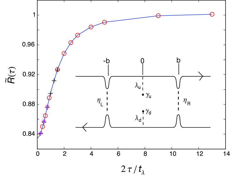
Figure 1: Reduction $\tilde{R}(\tau)$ of the imaginary time parity-parity correlation function due to coupling between edge and localized modes. Inset shows the interferometer with two localized Majorana modes $\gamma_{u}$, $\gamma_{d}$ coupled to upper and lower edge, respectively. Data were numerically obtained for an interferometer of size $b=t_{\lambda}/4$ and total system size $L+b=10.5t_{\lambda}$, where $t_{\lambda}^{-1}$ is the characteristic decay rate of localized modes. Data points are shown for $a/t_{\lambda}=0.005$ (full line with open circles), $a/t_{\lambda}=0.0025$ (plus signs), and $a/t_{\lambda}=0.00125$ (asterisks), where $a$ denotes the lattice constant.

In order to analyze the strong coupling limit with either $t_{b}$ or $t_{V}$ of the order of $t_{\lambda}$, we numerically study a lattice version of our model futurepaper . We start with a tight-binding Hamiltonian for one-dimensional complex fermions without the localized modes: $H\ =\ -v_{m}a^{-1}\sum_{j}(c_{j+1}^{\dagger}c_{j}\ +\ h.c.)$. Here, $a$ is the lattice constant, and the operators obey the usual anti-commutation relations $\{c_{i}^{\dagger},c_{j}\}=\delta_{ij}$. We study the model at half filling with a Fermi wave vector $k_{F}={\pi/2}$. The fermions created by $c_{j}^{\dagger}$ can be decomposed into two Majorana species

$$\gamma_{j}\ =\ e^{i{\pi\over 2}j}\ c_{j}\ +\ e^{-i{\pi\over 2}j}\ c_{j}^{\dagger}\ ,\ \ \ \ \ \tilde{\gamma}_{j}\ =\ {1\over i}\big{(}e^{i{\pi\over 2}j}\ c_{j}\ -\ e^{-i{\pi\over 2}j}\ c_{j}^{\dagger}\big{)}\,.$$

We define continuum fermions, using $\gamma_{j}$ alone, via

$$\Psi^{u,d}(ja) = {1\over\sqrt{a}}\sum_{j^{\prime}}(\pm 1)^{j^{\prime}}f(j-j^{\prime})\gamma_{j^{\prime}}\ \ ,$$ (10)

where $f(j)$ is a Gaussian with a width large compared to the lattice spacing and subject to the normalization $\sum_{j}f(j)=\sqrt{\pi}$. Using this mapping one can now include the coupling to the localized modes as in Eq. (1).

The parity operator for a set of lattice sites $\{j\}$ can be written as the product over sites of operators $2c_{j}^{\dagger}c_{j}-1=i\gamma_{j}\tilde{\gamma}_{j}$. The parity operator for the localized modes has a similar form. The expectation value of any such product, at the same or different times, can be evaluated, using Wick’s theorem, as the Pfaffian of a matrix whose elements are the pair correlation functions of operators on different sites, including the localized modes where appropriate. As the Hamiltonian is a sum $H=H_{\gamma}+H_{\tilde{\gamma}}$, the $\tilde{\gamma}$ species contributes a factor to the parity expectation value which is the same whether the localized modes are present or not. Thus we may ignore the $\tilde{\gamma}$ modes in evaluating the reduction factor. In this way, the lattice form for the edge parity for a region $[x_{1},x_{2}]$ becomes

$$P_{edge}(x_{1},x_{2})\ =\ \prod_{x_{1}\leq x_{j}\leq x_{2}}\sqrt{i}\;\gamma_{j}\ \ .$$ (11)

To calculate the reduction factor at time $t$ we will need to evaluate expectation values of products like $\langle P_{edge}(-L,-b;t)P_{edge}(-L,b;0)i\gamma_{u}\gamma_{d}\rangle\,,$ where $-L\ll-|t|$ is a point far to the left of the origin. In the absence of bulk-edge coupling, the pair correlation function for two lattice points at equal times is

$$\langle i\gamma_{j}\gamma_{k}\rangle_{0}\ =\ {1\over\pi}{1\over j-k}\ \Big{[}1\ -\ e^{-i\pi(j-k)}\Big{]}\ \ .$$ (12)

The two terms in brackets arise from the right-moving upper edge and left-moving lower edge, respectively. With non-zero bulk-edge coupling, the correlation functions $\langle i\gamma_{j}\gamma_{k}\rangle$ and $\langle i\gamma_{j}\gamma_{u(d)}\rangle$ can be calculated analytically in the continuum limit (i.e., for points not too close to the origin) for the same and for different times. A full lattice calculation can be carried out numerically, but it is time-consuming for large lattices. We have found that the short-distance errors introduced by using continuum correlation functions only lead to an error in the Pfaffian by a factor $c_{\lambda}$ that depends on $a/t_{\lambda}$ but is independent of the interferometer size $b$ and the time difference $t$. The numerical results presented in Fig. 1 were obtained using the continuum correlation functions and corrected by the factor $c_{\lambda}$ . The numerical value of $c_{\lambda}$ can be obtained most easily by considering equal time correlation functions. As a check, we note that results for different values of $a/t_{\lambda}$ obtained with this numerical technique deviate less than 0.3 % from each other, as shown in Fig. 1.

Fig. 1 displays the imaginary time reduction factor $\tilde{R}(\tau)$ for intermediate and strong coupling, for an interferometer size $b=t_{\lambda}/4$. $\tilde{R}(\tau)$ is related to the real time reduction factor via the analytic contiuation $R(t)=\tilde{R}(\tau\to it+\delta)$. The reduction factor $\tilde{R}(\tau)$ monotonically increases with increasing time. At $\tau\approx t_{\lambda}$, there is a crossover from parity reduction determined by the interferometer size $b=t_{\lambda}/4$ to parity reduction determined by the time. At large times $\tilde{R}(\tau)$ seems to saturate at a value of one, implying that its analytic continuation $R(t)$ saturates near one as well. Note that when $R(t)=1$ the visibility of the interference is the same as it would have been in the absence of the two bulk quasiparticles. Similar results are expected if we have one strongly coupled localized mode inside the interferometer path, and a second localized mode, of arbitrary coupling, outside the interferometer. We attribute the re-emergence of the interference as the bulk-edge coupling gets strong to the correlations that develop between the occupation of the fermionic mode associated with the two quasi-particles and the occupation of the region of the edge at a distance $v_{m}t_{\lambda}$ from the coupling point. Each of these occupations strongly fluctuates due to the coupling, but their fluctuations are strongly correlated.

In conclusion, we have found that when the coupling between the Majorana mode associated with a localized $e*=e/4$ charged quasiparticle and an adjacent edge is sufficiently strong, so that the characteristic tunneling time $t_{\lambda}$ is short compared to the time scale $t_{V}=\hbar e^{*}/V$ set by the voltage, it appears as if the localized quasiparticle has become part of the edge. Specifically, for an interference path enclosing the quasiparticle, the interference visibility should have essentially the same strength as if the quasiparticle were not there. For weak coupling, the time-averaged interference intensity is reduced, by a factor which is $\propto(t_{V}/t_{\lambda})\log^{2}(t_{\lambda}/t_{V})$ in the case where there are two localized quasiparticles inside the loop, coupled respectively to the two edges with similar strength.

Acknowledgments: We would like to thank B.J. Overbosch and X.-G. Wen for fruitful discussions. This work was supported in part by the Heisenberg program of DFG, by NSF grant DMR-0541988, the US-Israel BSF, the Minerva foundation, and the Israel Science Foundation.

References

- (1) S. Das Sarma, M. Freedman, C. Nayak, S. H. Simon, and A. Stern, arXiv:0707.1889.
- (2) S. Das Sarma, M. Freedman, C. Nayak, Phys. Rev. Lett. 94, 166802 (2005).
- (3) A. Stern and B. I. Halperin, Phys. Rev. Lett. 96, 016802 (2006).
- (4) P. Bonderson, A. Kitaev, and K. Shtengel, Phys. Rev. Lett. 96, 016803 (2006).
- (5) E. Fradkin, C. Nayak, A. Tsvelik, and F. Wilczek, Nucl. Phys. B516, 704 (1998).
- (6) C. de C. Chamon, et al., Phys. Rev. B 55, 2331 (1997).
- (7) B. J. Overbosch and X.-G. Wen, arXiv:0706.4339.
- (8) P. Fendley, M.P.A. Fisher, and C. Nayak, Phys. Rev. B 75, 045317 (2007).
- (9) See, for example, Conformal Field Theory, P. Di Francesco, P. Mathieu, and D. Sénéchal, Springer-Verlag (1997).
- (10) A different gauge choice would have given us the parity of the number of electrons to the right of .
- (11) E. Ardonne and E.-A. Kim, arXiv:0705.2902.
- (12) Since our reduction factor R(t) is a product of separate contributions from the upper and lower edges, we can infer from one of these the result for a single localized mode.
- (13) More details will be given in a future paper.