1 Introduction

There is a well known way of obtaining the General Relativity Lagrangian which is associated with the name of Feynman [8], although many other scientists have contributed to it, starting with Kraichnan [11] . The idea is the following: if one starts from the Fierz-Pauli Lagrangian (which describes free spin two particles in Minkowski space)

$$L_{FP}=\frac{1}{4}\partial_{\mu}h^{\nu\rho}\partial^{\mu}h_{\nu\rho}-\frac{1}{2}\partial_{\mu}h^{\mu\rho}\partial_{\nu}h^{\nu}_{\rho}+\frac{1}{2}\partial^{\mu}h\partial^{\rho}h_{\mu\rho}-\frac{1}{4}\partial_{\mu}h\partial^{\mu}h$$ (1)

where all indices are raised and lowered with the flat Minkowski metric; in particular:

$$h^{\mu\nu}\equiv\eta^{\mu\alpha}\eta^{\nu\beta}h_{\alpha\beta}$$

$$h\equiv\eta^{\alpha\beta}h_{\alpha\beta}$$ (2)

it so happens that the equations of motion $D^{FP}_{\mu\nu}\equiv\frac{1}{2}\frac{\delta S_{FP}}{\delta h^{\mu\nu}}$ are transverse, i.e.

$$\partial^{\mu}D^{FP}_{\mu\nu}=0$$ (3)

In order to coupling the graviton field $h_{\mu\nu}$ to an scalar field $\phi$, say, it is natural to try the coupling to the conserved energy-momentum tensor (suitably symmetrized if needed, for example using the Belinfante technique), that is

$$L_{I}\equiv h^{\mu\nu}T_{\mu\nu}$$ (4)

But when this term is added to the matter Lagrangian in an freely falling inertial frame

$$L^{0}_{m}=\frac{1}{2}\eta^{\mu\nu}\partial_{\mu}\phi\partial_{\nu}\phi-V(\phi)$$ (5)

the former energy-momentum tensor is no longer conserved, and the gravitational equation of motion is inconsistent. This leads to a series of modifications that eventually end up in the Hilbert Lagrangian. The quickest path to is probably Deser’s, [7] using a first order formalism. The aim of the present paper is to explore what room is left in this argument for less symmetric nonlinear completions, notably the ones we dubbed TDiff, which are invariant under coordinate transformations whose jacobian enjoys unit determinant. These have been explored in [4], where further references can be found.

2 The linear approximation

It is nevertheless clear that given a consistent theory (such as General Relativity itself) its linear part in any analytic expansion should be consistent as well (up to linear order). The object of our concern in the present paper will be the linear deviations from flat Minkowski space, i.e.

$$g_{\mu\nu}=\eta_{\mu\nu}+\kappa h_{\mu\nu}$$ (6)

where $\eta_{\mu\nu}$ is the Minkowski metric, and $\kappa^{2}\equiv 8\pi G$. This equation is taken to be an exact one; it can be looked at as the definition of $h_{\mu\nu}$.

Now, it is a fact of life that $l_{P}\equiv\kappa\sqrt{\frac{\hbar}{c^{3}}}$ has got dimensions of length, and that $M_{P}\equiv\frac{\sqrt{\hbar c}}{\kappa}$ enjoys dimensions of mass. The value of Newton’ s constant indicates that at the scale of terrestial experiments, $M_{P}\sim 10^{19}GeV$. This means that the field $h_{\mu\nu}$ enjoys the proper canonical dimension (one) of a four-dimensional gauge field.

The inverse metric is defined as a formal power series:

$$g^{\mu\nu}=\eta^{\mu\nu}-\kappa h^{\mu\nu}+\kappa^{2}h^{\mu}_{\sigma}h^{\sigma\nu}-\kappa^{3}h^{\mu\sigma}h_{\sigma\rho}h^{\rho\nu}+o(\kappa^{4})$$ (7)

Diffeomorphisms with infinitesimal parameter $\xi^{\mu}$ act on the full metric as

$$\delta g_{\mu\nu}=\pounds(\xi)g_{\mu\nu}$$ (8)

whereas in terms of the fluctuations

$$\delta h_{\mu\nu}=\xi^{\rho}\partial_{\rho}h_{\mu\nu}+\frac{1}{\kappa}\left(\partial_{\mu}\xi_{\nu}+\partial_{\nu}\xi_{\mu}\right)+h_{\mu\alpha}\partial_{\nu}\xi^{\alpha}+h_{\alpha\nu}\partial_{\mu}\xi^{\alpha}$$ (9)

This is, again, an exact formula, in the sense that there are no $\kappa$ corrections to it.

The symmetry as above, without any restrictions, is the one corresponding to General Relativity, and in the present paper will be referred to simply as Diff. When the vector $\xi^{\alpha}$ is restricted to

$$\partial_{\alpha}\xi^{\alpha}=0$$ (10)

the symmetry is broken to what we call T(ransverse)Diff [6].

The total action is then defined by

$$S=\frac{1}{2}S_{h}+S_{m}$$ (11)

Here $S_{h}$ represents the purely gravitational sector, which is the most general Lorentz invariant dimension four operator that can be written with the field $h_{\alpha\beta}$, and its derivatives. It can be parametrized by a string of constants, namely the ones associated with the kinetic energy, $c_{i}$,$i=1\ldots 3$ and the ones associated to the potential energy for the fluctuations, which is the most general quartic potential in the fluctuations $h_{\alpha\beta}$, namely, $\lambda_{i}$, $i=1\ldots 11$. The overall scale of the potential energy is related to the cosmological constant, $\Lambda\equiv M_{D}^{4}$. Cosmological observations seem to favor the tiny value $M_{D}\sim 10^{-3}eV$.

$$S_{h} \equiv \int d^{4}x\left(\frac{1}{4}\partial_{\mu}h^{\nu\rho}\partial^{\mu}h_{\nu\rho}-\frac{c_{1}}{2}\partial_{\mu}h^{\mu\rho}\partial_{\nu}h^{\nu}_{\rho}+c_{2}\frac{1}{2}\partial^{\mu}h\partial^{\rho}h_{\mu\rho}-c_{3}\frac{1}{4}\partial_{\mu}h\partial^{\mu}h+\right.$$ (12)

$$M_{D}^{4}\left(1+\frac{1}{2M_{P}}\lambda_{1}h+\frac{1}{8M_{P}^{2}}\left(\lambda_{2}h^{2}-2\lambda_{3}h_{\alpha\beta}h^{\alpha\beta}\right)+\right.$$

$$\left.\left.\frac{1}{48M_{P}^{3}}\left(\lambda_{4}h^{3}+8\lambda_{5}h_{\mu\nu}h^{\nu\rho}h_{\rho}^{\mu}-6\lambda_{6}hh_{\alpha\beta}h^{\alpha\beta}\right)+\right.\right.$$

$$\left.\left.\frac{1}{384M_{P}^{4}}\left(\lambda_{7}h^{4}-12\lambda_{8}h^{2}h_{\alpha\beta}h^{\alpha\beta}+32\lambda_{9}hh_{\alpha\beta}h^{\beta\gamma}h_{\gamma}^{\alpha}-\right.\right.\right.$$

$$\left.\left.\left.48\lambda_{10}h_{\alpha\beta}h^{\beta\gamma}h_{\gamma\delta}h^{\delta\alpha}+12\lambda_{11}\left(h_{\alpha\beta}h^{\alpha\beta}\right)^{2}\right)\right)\right)$$

Let us remark, first of all, that the structure of the symmetry transformations of both Diff and TDiff is such that terms in the Lagrangian of $O(M_{P}^{-n})$ are related to terns of both $O(M_{P}^{-n})$ as well as, because of the abelian part, terms of $O(M_{P}^{-n+1})$. This means that in the variations of the kinetic energy part we can keep only the piece in $M_{P}$ , since the other part ($O(M_{P}^{0})$) of the variation should cancel with the $M_{P}$ contribution to the kinetic operators of order $O(\frac{1}{M_{P}})$, which we have not considered. The only piece we can consistently consider there is then the Fierz-Pauli abelian part given by

$$\delta h_{\mu\nu}=M_{p}\left(\partial_{\mu}\xi_{\nu}+\partial_{\nu}\xi_{\mu}\right)$$ (13)

The situation is different, however, in the potential energy piece. In order to cancel the Fierz-Pauli variation of the $O(M_{P}^{-2})$ term, it is necessary to consider the $O(M_{P}^{0})$ variation of the $O(\frac{1}{M_{P}})$ term. This means that the full action is invariant under the full variation (9) up to dimension five operators (which means $O(\frac{1}{M_{P}})$ in the kinetic energy part, and $O(\frac{1}{M_{P}^{-5}})$ in the potential energy piece).

Under those provisos, TDiff needs that

$$\lambda_{1}=\lambda_{3}=\lambda_{5}=\lambda_{10}$$

$$\lambda_{2}=\lambda_{6}=\lambda_{9}=\lambda_{11}$$

$$\lambda_{4}=\lambda_{8}$$ (14)

The most general TDiff invariant potential depends on four arbitrary parameters. In some studies it is frequent to restrict the gravitational equations of motion to the linear approximation; this means quadratic terms in the gravitational lagrangian. From a field theoretical viewpoint there is no reason lo leave away any relevant (in the renormalization group sense) operators.

• Let us first consider the case $\lambda_{i}=0\quad\forall i$. This corresponds to vanishing cosmological constant in general relativity. First of all, TDiff enforces $c_{1}=1$.

  Besides, there are two exceptional values, namely $c_{i}=1,\forall i$, when TDiff is enhanced to full Diff . This is the only combination for which the wave operator is transverse.

  $$\frac{1}{2}\frac{\delta S_{h}}{\delta h^{\alpha\beta}} \equiv D^{h}_{\alpha\beta}=-\frac{1}{4}\Box h_{\alpha\beta}+\frac{c_{1}}{4}\left(\partial_{\rho}\partial_{\alpha}h_{\beta}^{\rho}+\partial_{\rho}\partial_{\beta}h^{\rho}_{\alpha}\right)-\frac{c_{2}}{4}\left(\eta_{\alpha\beta}\partial_{\mu}\partial_{\nu}h^{\mu\nu}+\partial_{\alpha}\partial_{\beta}h\right)+$$ (15)

  $$+\frac{c_{3}}{4}\Box h\,\eta_{\alpha\beta}$$

  Indeed

  $$\partial^{\alpha}D^{h}_{\alpha\beta}=\frac{c_{1}-1}{4}\Box\partial^{\alpha}h_{\alpha\beta}+\frac{c_{1}-c_{2}}{4}\partial_{\beta}\partial_{\rho}\partial_{\sigma}h^{\rho\sigma}+\frac{c_{3}-c_{2}}{4}\Box\partial_{\beta}h$$ (16)

  By the way, it is worth noticing that the metric condition

  $$\nabla_{\mu}g_{\alpha\beta}=0$$ (17)

  is identically satisfied to $o(\kappa)$ and poses no restriction on $h_{\mu\nu}$.

• The other remarkable value is $c_{1}=1,\,c_{2}=\frac{1}{2},\,c_{3}=\frac{3}{8}$ where the symmetry is enhanced with a Weyl invariance, denoted by WTDiff, and the wave operator is traceless in the absence of cosmological constant. To be specific,

  $$\eta^{\mu\nu}D^{h}_{\mu\nu}=\left(c_{3}-\frac{c_{2}+1}{4}\right)\Box h+\left(c_{2}-\frac{c_{1}}{2}\right)\partial_{\mu}\partial_{\nu}h^{\mu\nu}$$ (18)

  The analysis in [4] shows that these two are the only instances where only spin two is present, with no scalar contamination.

• Let us now consider the effect of $\lambda_{i}\neq 0$. First of all, Diff invariance is recovered when $\lambda_{i}=1\quad\forall i$. Curiously enough, as such, and in the quadratic approximation, the term

  $$m_{1}^{2}\equiv\frac{M_{D}^{4}}{M_{p}^{2}}\lambda_{3}$$ (19)

  as well as

  $$m_{2}^{2}\equiv\frac{M_{D}^{4}}{2M_{p}^{2}}\lambda_{2}$$ (20)

  do have the interpretation of masses.

  Only when the background around which we perturb is not flat, but a constant curvature space, with metric $\bar{g}_{\mu\nu}$, do these paramerers recover the meaning of cosmological constant. In that case it is mandatory to substitute all derivatives by background covariant derivatives, i.e.,

  $$\partial_{\alpha}h_{\mu\nu}\rightarrow\bar{\nabla}_{\alpha}h_{\mu\nu}$$ (21)

  and to raise and lower indices using the corresponding background metric:

  $$h^{\mu\nu}\equiv\bar{g}^{\mu\alpha}\bar{g}^{\nu\beta}h_{\alpha\beta}$$ (22)

• Let us study now consistency of the coupling, which was the main motivation of this work. The matter Lagrangian has been denoted by $S_{m}$. Up to dimension five operators for a scalar field, which in a free falling locally inertial reference system has lagrangian

  $$L^{0}_{m}=\frac{1}{2}\eta^{\mu\nu}\partial_{\mu}\phi\partial_{\nu}\phi-V(\phi)$$ (23)

  assuming a $\mathbb{Z}_{2}$ symmetry

  $$\phi\rightarrow-\phi$$ (24)

  the allowed matter operators when a gravitational field is present can be parameterized by three constants, $\mu_{1}\ldots\mu_{3}$:

  $$L_{m}=\frac{1}{2}\eta^{\mu\nu}\partial_{\mu}\phi\partial_{\nu}\phi-V(\phi)+\frac{1}{M_{P}}\left(-\frac{\mu_{1}}{2}h^{\mu\nu}\partial_{\mu}\phi\partial_{\nu}\phi+\mu_{2}\frac{1}{4}h\eta^{\mu\nu}\partial_{\mu}\phi\partial_{\nu}\phi-\mu_{3}\frac{h}{2}V(\phi)\right)$$ (25)

  Remember that the variation of a scalar field is

  $$\delta\phi=\xi^{\mu}\partial_{\mu}\phi$$ (26)

  In order to enjoy TDiff invariance, it is necessary that $\mu_{1}=1$. Diff invariance needs in addition that $\mu_{2}=\mu_{3}=1$. The matter equations of motion are

  $$\frac{\delta S_{m}}{\delta\phi}=-\Box\phi-V^{\prime}(\phi)+\frac{1}{M_{p}}\left(\mu_{1}\partial_{\alpha}\left(h^{\alpha\beta}\partial_{\beta}\phi\right)-\frac{\mu_{2}}{2}\partial_{\alpha}\left(h\partial^{\alpha}\phi\right)-\mu_{3}\frac{h}{2}V^{\prime}(\phi)\right)$$ (27)

  and the gravitational equations

  $$\frac{\delta\left(\frac{S_{h}}{2}+S_{m}\right)}{\delta h_{\mu\nu}}=D^{h}_{\mu\nu}-\frac{1}{M_{p}}\left(\frac{1}{2}\mu_{1}\partial_{\mu}\phi\partial_{\nu}\phi+\frac{1}{2}\left(\mu_{3}V(\phi)-\frac{\mu_{2}}{2}(\partial_{\alpha}\phi)^{2}\right)\eta_{\mu\nu}\right)$$ (28)

  There is generically no problem of consistency, except in the two exceptional cases.

  First of all, when $S_{h}$ has extended Diff symmetry, and consequently a transverse wave operator, this forces $S_{m}$ to have the same Diff symmetry through the linear expansion of the $\sqrt{|g|}$ term; otherwise consistency of the coupling enforces extra condictions on the matter, a very weird situation indeed (i.e. Bianchi identities are still valid on the gravitational side, so that by consistency the same identities must hold true on the matter side as well). Nevertheless, it is not fully devoid of interest to study the situations in which there are exceptions to this rule; this we did in a previous work [3].

• When there is WTDiff symmetry, it is clear that the matter lagrangian should also be scale invariant in order for the corresponding energy-momentum to be traceless. In our example, this corresponds to $\mu_{1}=2\mu_{2}$ and $\mu_{3}=0$.

• There are models in which Diff invariance in the matter sector is reached using in the volume element some other scalar density, such as the square root of the determinant of a matrix built out of fields and their derivatives (as in the very interesting ones proposed in [9]) instead of the $\sqrt{|g|}$ term implicit in the metric volume element. The tensor that appears as the source of gravity in Einstein’s equations is covariantly conserved thanks to the equations of motion of the fields in the scalar density. Of course that tensor is not the usual energy-momentum tensor of General Relativity, which now is not conserved. The reason is that in order for the Rosenfeld energy-momentum tensor to be equivalent to the canonical Belinfante one what is needed is not only Diff invariance, but also the standard metric volume element [5]. This topic seems worthy of some further investigation.

3 Observational constraints

In this section we will outline the way in which one can constraint the space of paramaters of the linearized theory (i.e. $c_{i}$, $\mu_{i}$ and $\lambda_{i}$) using experimental results on deviations from Newton’s inverse square law. For simplicity we will illustrate with a very particular example so no definite conclusions can be drawn concerning the viability of this kind of models.

Detailed computations of the propagators can be found in [4], where the authors considered a gravitational Lagrangian (12) with all $\lambda_{i}=0$ except $m_{2}^{2}\equiv\frac{M_{D}^{4}}{2M_{p}^{2}}\lambda_{2}$ which has the interpretation of a mass for the scalar part of the graviton, present generically in this kind of models with TDiff invariance. It turns out that for a conserved energy-momentum tensor coupled to gravity in the form

$$L_{I}=\frac{1}{2}h_{\mu\nu}\left(\kappa_{1}T^{\mu\nu}+\kappa_{2}\eta^{\mu\nu}T\right)$$ (29)

then in momentum space the interaction is

$$L_{I}=\kappa_{1}^{2}\left[T^{*}_{\mu\nu}T^{\mu\nu}-\frac{1}{2}|T|^{2}\right]\frac{1}{k^{2}}-\left(\kappa_{2}+\frac{1-c_{2}}{2}\kappa_{1}\right)^{2}\frac{|T|^{2}}{\Delta ck^{2}-m_{2}^{2}}$$ (30)

where we have defined

$$\Delta c=c_{3}-\frac{1}{2}+c_{2}-\frac{3}{2}c_{2}^{2}$$ (31)

with the constraint $\Delta c<0$ because of unitarity [4]. The first term corresponds to the usual spin 2 exchange while the second one is an additional massive scalar interaction. Let us turn our attention to a particular example, namely the matter Lagrangian (25). Unfortunately the corresponding energy momentum tensor is not conserved. However, a conserved tensor can be defined as

$$\Theta_{\mu\nu} \equiv T_{\mu\nu}-\frac{1}{2}\eta_{\mu\nu}\left(\frac{1-\mu_{2}}{2}(\partial_{\rho}\phi)^{2}+(\mu_{3}-1)V(\phi)\right)+O(\frac{1}{M_{p}})=$$ (32)

$$= \frac{1}{2}\partial_{\mu}\phi\partial_{\nu}\phi-\frac{1}{2}\eta_{\mu\nu}\left(\frac{1}{2}(\partial_{\rho}\phi)^{2}-V(\phi)\right)+O(\frac{1}{M_{p}})$$

In the particular case that $\mu_{3}=2\mu_{2}-1$ (which includes the Diff invariant Lagrangian) our energy-momentum tensor can be written in terms of the new one and its trace in such a way that the coupling $M_{p}^{-1}h_{\mu\nu}T^{\mu\nu}$ is of the form (29) with

$$\kappa_{1}=\frac{2}{M_{p}}$$

$$\kappa_{2}=\frac{\mu_{2}-1}{M_{p}}$$ (33)

Now we can apply directly the preceeding results and study experimental constraints to this model. The exchange of additional massive scalar degrees of freedom produces a Yukawa like potential which is usually parametrized as [1]

$$V(r)\sim\frac{1}{r}\left(1+\alpha e^{-\frac{r}{\lambda}}\right)$$ (34)

The parameter $\alpha$ is then the ratio between the spin 2 and the scalar couplings, in our particular case

$$\alpha=-\frac{\left(\kappa_{2}+\frac{1-c_{2}}{2}\kappa_{1}\right)^{2}}{\Delta c\,\,\kappa_{1}^{2}}=-\frac{\left(\mu_{2}-c_{2}\right)^{2}}{4\,\Delta c}$$ (35)

While $\lambda$ gives the range of the interaction, or equvalently the mass of the scalar exchanged

$$\lambda^{2}=\frac{\Delta c}{m_{2}^{2}}$$ (36)

Notice that one has to impose $m_{2}^{2}<0$ since as we have said absence of ghosts requires $\Delta c<0$.

There are important constraints on the strength of hypothetical Yukawa interactions for a wide range of $\lambda$. Through (35) and (36) it is then possible to constraint the space of parameters of the linearized theory. We will use figures 4, 5 and 9 of reference [1], which show regions allowed and excluded for $\alpha$ corresponding to $\lambda$ in the ranges $10^{-9}$m-$10^{-6}$m, $10^{-6}$m-$10^{-2}$m and $10^{-2}$m-$10^{14}$m respectively. Since we are just interested in general behaviours and not in accurate results we will approximate the experimental curves by straight lines. The original plots are in logarithmic scale so we have experimentally allowed regions of the form

$$|\alpha|<k\,\lambda^{a}$$ (37)

We just have to substitute this expresion into (35) to get bounds for our parameters. There are however four parameters to play with ($\mu_{2}$, $m_{2}^{2}$, $c_{2}$ and $c_{3}$). First, it is interesting to see the order of magnitude for the mass once we fix the values of $c_{2}$ and $c_{3}$. The result is ploted in Fig.1. It can be seen that greater values for the mass are favoured, being the lower bound around $|m_{2}^{2}|\sim 5\times 10^{11}\mathrm{m}^{-2}\sim 0.02\,\,\mathrm{eV}^{2}$, and that the allowed region rapidly decreases with $|\Delta c|$.

Figure 1: The shadowed region shows experimentally allowed values for $|m_{2}^{2}|$ (in $m^{-2}$) and $\mu_{2}$ for given values of $c_{2}$ and $c_{3}$, expressed in terms of $\Delta c$, and in the range $\lambda\in$ $10^{-9}$m-$10^{-6}$m.

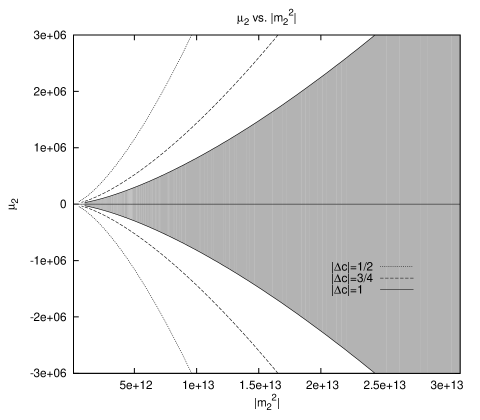
Another possibility is to fix $|m_{2}^{2}|$ and $\mu_{2}$ and see, in the plane ($c_{2}$,$c_{3}$), how far from Diff invariance (which corresponds to $c_{2}=c_{3}=1$) can we move away. Remember that we also have to take into account the restriction $\Delta c<0$. For the first range, $\lambda\in 10^{-9}$m-$10^{-6}$m there is no hope of seeing an experimental curve that appreciably deviates from the parabola $\Delta c=0$ because of (36) and the tiny values of $\lambda$. Increasing $|m_{2}^{2}|$ does increase the allowed region, which is between both curves, but does not produce a plot in which the curves are visibly separate. It can be understood if we realise that increasing the mass also increases $c_{3}$ on the parabola through $c_{2}$ and (35)-(36). An approximate definition of the separation could be

$$Sep\sim\frac{(c_{3})_{par}-(c_{3})_{cur}}{(c_{3})_{par}}=\frac{\lambda^{2}|m_{2}^{2}|}{\frac{1}{2}-c_{2}(\lambda,m_{2})+\frac{3}{2}c_{2}(\lambda,m_{2})^{2}}$$ (38)

where $(c_{3})_{par}$ and $(c_{3})_{cur}$ means the value of $c_{3}$ on the parabola and the experimental curve respectively. For the first experimental range one has $Sep<<1$ independently of the mass and in the whole interval. The other two cases do not have that property, which is of course related also with the particular values of $k$ and $a$ in (37). Examples of resulting plots are Figs.2, 3 and 4.

Once again the experiment prefers greater values for the mass. All the plots have $\mu_{2}=0$, other values just move the experimental curve along the parabola, but the qualitative result remains unchanged.

Figure 2: Experimentally allowed region in the plane ($c_{2}$,$c_{3}$), for a couple of values of the mass, in the range $\lambda\in 10^{-6}$m-$10^{-2}$m. The plot is restricted to the zone where the curve appreciably deviates from the parabola $\Delta c=0$.

Figure 3: Experimentally allowed region in the plane ($c_{2}$,$c_{3}$), for a couple of values of the mass, in the range $\lambda\in 10^{-2}$m-$10^{14}$m. We only show the positive $c_{2}$ branch. The parabola is indistinguisable from the $c_{2}$ axis.

Figure 4: Experimentally allowed region in the plane ($c_{2}$,$c_{3}$) and in the range $\lambda\in 10^{-2}$m-$10^{14}$m for a very tiny mass. That allows us to see the parabola, which was hidden in the previous figure. We only show the zone closest to the $c_{3}$ axis.

4 Conclusions

In this paper we have studied at the linearized level the viability of gravity models with a restricted symmetry, both from the theoretical and observational points of view. While the existing observational constraints on additional Yukawa like gravitatory interactions do not seem to be a major obstacle, a consistency problem has been identified. At the non linear level it appeared as an integrability condition on Einstein’s equations [3]. Here we turned our attention to the linear level in order to see if the problem could be avoided, and if so in what type of more clever non linear completions. The main conclusion is that it is not generically possible to couple matter (i.e., with an arbitrary equation of state) to gravitation in such a way that this coupling has a restricted symmetry only (what has been called TDiff) whereas the purely gravitational sector enjoys a higher symmetry, namely the standard Diff invariance, or an additional Weyl symmetry (WTDiff). That this is possible in some restricted cases has been already found in a previous paper [3].

The condition for arbitrary TDiff matter to be able to couple to Diff gravity without restrictions can be stated somewhat more formally by saying that the Rosenfeld (metric) energy-momentum tensor has got to be equivalent to the Belinfante canonical form.

On the other hand, there is a widespread urban legend asserting that unimodular theories are equivalent to General Relativity with a cosmological constant. Specific calculations both here and in our previous paper [3] have proven it to be groundless. It is a fact that in some TDiff models there is no exponential expansion at all which is well known to be the benchmark of a (positive) cosmological constant in General Relativity. Therefore, that models provide a counterexample to the statement above.

Nevertheless, as with all legends, there is some partial truth in it. The equations of motion of the example in [3] correspond to $c_{1}=c_{2}=c_{3}=\mu_{1}=1$ and $\mu_{2}=\mu_{3}=\lambda_{i}=0$, that is

$$D^{FP}_{\alpha\beta}=\frac{1}{M_{P}}\partial_{\alpha}\phi\partial_{\beta}\phi$$ (39)

whereas the linear equations of General Relativity with cosmological constant read:

$$D^{FP}_{\alpha\beta}+\frac{\lambda M_{P}^{3}}{4}\eta_{\alpha\beta}=\frac{1}{M_{P}}\left(\partial_{\alpha}\phi\partial_{\beta}\phi+\frac{1}{2}\left(V(\phi)-\frac{1}{2}(\partial_{\rho}\phi)^{2}\right)\eta_{\alpha\beta}\right)$$ (40)

Now, the equations (39) are inconsistent as such, in the sense that only a subsector of the theory, namely, the one that obeys

$$V-\frac{1}{2}(\partial_{\rho}\phi)^{2}=C$$ (41)

can be coupled to gravitation. There are many sectors of matter in a freely falling inertial system that do not obey this restriction. Actually, together with energy conservation, the aforementioned equation implies that both the kinetic and potential energy ought to be constant:

$$2V(\phi)=E+C$$

$$(\partial_{\rho}\phi)^{2}=E-C$$ (42)

It is clear that for a scalar field in flat space most initial conditions lead to configurations that violate those equations. This would mean that an inconsistency would show up once a gravitational field is turned on, however weak. More formally, something very strange should happen when changing the reference frame from an inertial (freely falling one) to another in which a gravitational field is present.

Those are the reasons what we say that the coupling is generically inconsistent. Let us accept nevertheless, for the sake of the argument, that physics is so restricted. Then a glance at the equations (40) of General Relativity shows that they are indeed equivalent to (39) provided we identify

$$\lambda\equiv\frac{2C}{M_{P}^{4}}$$ (43)

But this is only due to our choice of the arbitrary constants, and under the asumption that the coupled sector is only the one that obeys (41), a deeply misterious condition from a General Relativistic perspective. In the general TDiff case the analogous condition to (41) is

$$-\frac{\mu_{2}-1}{2}(\partial_{\rho}\phi)^{2}+(\mu_{3}-1)V(\phi)=C$$ (44)

and the system is not equivalent to General Relativity with a cosmological constant.

References

- [1] E. G. Adelberger, B. R. Heckel and A. E. Nelson, “Tests of the gravitational inverse-square law,” Ann. Rev. Nucl. Part. Sci. 53 (2003) 77 [arXiv:hep-ph/0307284].
- [2] E. Alvarez, “Quantum Gravity: A Pedagogical Introduction To Some Recent Results,” Rev. Mod. Phys. 61 (1989) 561.
- [3] E. Alvarez and A. F. Faedo, “Unimodular cosmology and the weight of energy,” Phys. Rev. D 76 (2007) 064013 [arXiv:hep-th/0702184].
-
[4]
E. Alvarez, D. Blas, J. Garriga and E. Verdaguer,
“Transverse Fierz-Pauli symmetry,”
Nucl. Phys. B 756 (2006) 148
[arXiv:hep-th/0606019].
E. Alvarez, “Can one tell Einstein’s unimodular theory from Einstein’s general relativity?,” JHEP 0503 (2005) 002 [arXiv:hep-th/0501146]. - [5] S. V. Babak and L. P. Grishchuk, “The Energy-Momentum Tensor for the Gravitational Field,” Phys. Rev. D 61 (2000) 024038 [arXiv:gr-qc/9907027].
- [6] D. Blas, “Gauge symmetry and consistent spin-two theories,” J. Phys. A 40, 6965 (2007) [arXiv:hep-th/0701049].
- [7] S. Deser, “Self-interaction and gauge invariance,” Gen. Rel. Grav. 1 (1970) 9 [arXiv:gr-qc/0411023].
- [8] R. P. Feynman, F. B. Morinigo, W. G. Wagner and B. Hatfield, “Feynman lectures on gravitation,” Reading, USA: Addison-Wesley (1995) 232 p. (The advanced book program)
- [9] E. I. Guendelman and A. B. Kaganovich, “Dynamical measure and field theory models free of the cosmological constant problem,” Phys. Rev. D 60 (1999) 065004 [arXiv:gr-qc/9905029].
- [10] S. W. Hawking and G. F. R. Ellis, “The Large scale structure of space-time,” Cambridge University Press, Cambridge, 1973
- [11] R. H. Kraichnan, “Special-Relativistic Derivation of Generally Covariant Gravitation Theory,” Phys. Rev. 98 (1955) 1118
- [12] T. Ortin, “Gravity and strings,” (Cambridge University press, 2004)