The BOES spectropolarimeter for Zeeman measurements of stellar magnetic fields

Abstract

We introduce a new polarimeter installed on the high-resolution fiber-fed echelle spectrograph (called BOES) of the 1.8-m telescope at the Bohyunsan Optical Astronomy Observatory, Korea. The instrument is intended to measure stellar magnetic fields with high-resolution (R $\sim$ 60000) spectropolarimetric observations of intrinsic polarization in spectral lines. In this paper we describe the spectropolarimeter and present test observations of the longitudinal magnetic fields in some well-studied F-B main sequence magnetic stars ($m_{v}<8.8^{m}$). The results demonstrate that the instrument has a high precision ability of detecting the fields of these stars with typical accuracies ranged from about 2 to a few tens of gauss.

1 Introduction

The presence of intrinsic linear and circular polarizations in spectra of stellar objects provides an important information for diagnostics of their magnetism, wind surroundings, atmospheric inhomogeneities and other properties. For example, non-zero continuum linear polarization due to Thomson and Rayleigh scattering demonstrates the presence of non-symmetric patterns in the distribution of atmospheric or wind medium. The broad-band circular polarization as well as circular and linear polarizations in spectral lines exhibit information on the magnetic fields. The spectropolarimetric observation is therefore one of the most important tools for the experimental studies of stellar magnetism. To argue this statement, we start our consideration with a brief presentation of the most important historical results that have come to us from stellar spectropolarimetry.

• Magnetism of chemically peculiar main sequence stars. Strong magnetic fields up to several tens of kilogauss have been detected and studied on a large sample of chemically peculiar (CP) stars. In contrast to non-regular, localized magnetic fields of solar-type stars, statistical properties of the fields in CP stars and results of detailed modeling of field geometries in individual objects are generally consistent with the picture of smooth, roughly dipolar magnetic field, inclined with respect to the stellar axis of rotation (Landstreet, 2001).

• Magnetism of early-type pulsating and hot O-stars. Recently, comparatively weak regular magnetic fields have been found also in hot, massive $\beta$ Cep-type and some other pulsating stars (Hubrig et al., 2006), and O-type stars (Wade et al., 2006). Magnetic fields of these stars have also several morphological differences from magnetic fields of the Sun and other late-type stars.

• Magnetism of late-type, convective stars. Practically all manifestations of solar activity (chromosphere and corona, plages and spots, flares, etc.) are related to magnetic fields and their interaction with differential rotation and convection. Spectropolarimetric studies of fragmented and global magnetic fields make it possible to extend our knowledge about these processes to another solar-type and cooler convective stars.

  At the moment, the presence of global magnetic fields from a few to some tens of gauss has been established in convective stars of F9–M3 spectral types among I–V luminosity classes (Plachinda & Tarasova, 1999, 2000; Donati et al., 2003; Plachinda, 2004a, b; Petit et al., 2005).

This brief and, of course, not complete presentation illustrates the importance of spectropolarimetry as effective observational tool for studying the stellar magnetism.

Nowadays there is a large collection of portable (Eversberg et al., 1998, for instance) or stationary spectropolarimeters installed at different telescope. The 2–3 m class telescopes equipped with stationary spectropolarimeters are:

2.0m telescope, Pic du Midi, France
2.6m telescope, Crimea, Ukraine
2.6m Nordic telescope, La Palma, Spain
2.6m telescope, McDonald, USA
3.0m Italy national telescope, Italy
3.6m Canada-France-Hawaii telescope

Among the most known versions of spectropolarimeters installed at large telescopes are the imager/spectrograph/polarimeter FORS1 (Appenzeller et al., 1998) of the ESO, VLT; spectropolarimeters at the AAT (Bailey, 1989) and Keck (Goodrich et al., 1995). Very recently a low-resolution polarimeter was also installed at the 6-m Russian telescope (Naydenov et al., 2002). New magnetic weak-field main sequence and degenerate stars were detected/studied with these instruments (see, for instance, a review by Putney (1999) also Aznar Cuadrado et al. (2004); Valyavin et al. (2006); Wade et al. (2003) and references therein).

Recently designed high-resolution fiber-fed spectropolarimeters with intermediate class telescopes such as the MUSICOS (Donati et al., 1999), or ESPaDOnS (Manset & Donati, 2003) have demonstrated the best characteristics in obtaining the polarization spectra and measuring the stellar magnetic fields that created new generation of stellar spectropolarimeters. Typical accuracies of the field measurements with these instruments range from about 1 to a few tens of gauss that corresponds to the best instrumental level ever achieved with polarimeters of the 2–3m class telescopes (Wade et al., 2000, and references therein).

In this paper we introduce a new fiber-fed spectropolarimeter installed on the 1.8-m telescope of the Bohyunsan Optical Astronomy Observatory (BOAO) in Korea. This polarimeter provides high-resolution (R $\sim$ 60000) observations of all four Stokes Parameters and intended for high-precision Zeeman measurements of stellar magnetic fields with typical accuracies from about 1 to a few tens of gauss depending on the spectral characteristics of studied stars. Here we present the structure of this polarimeter and results of the longitudinal magnetic fields measurements for some well-studied magnetic stars. Observation of linear polarization is also available. However, due to poor weather conditions at the BOAO site and the presence of significant light pollution, observations of linear polarization are complicated and not so quite effective. Now, we are focused mainly on observations of circular polarization with this spectropolaimeter.

2 The BOES spectropolarimeter: basic principles and design.

The BOES (BoaO Echelle Spectrograph) is a high throughput, versatile, fiber-fed prism cross-dispersed echelle spectrograph installed at the 1.8-m telescope of the BOAO. Using a 2k x 4k CCD, the BOES can obtain a spectra simultaneously over a wide wavelength range of 3500 – 10500 $\AA$ with a throughput (resolution x slit width in arcsec.) around 125,000. It has nine fibers with core diameter from 80 to 300 $\mu$m, corresponding field of views and resolutions ($\lambda$/$\Delta\lambda$) are 1.1 $\sim$ 4.3 arcsec. and 30000 $\sim$ 90000 respectively.

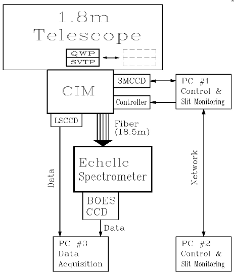
Figure 1: The block diagram of the BOES.

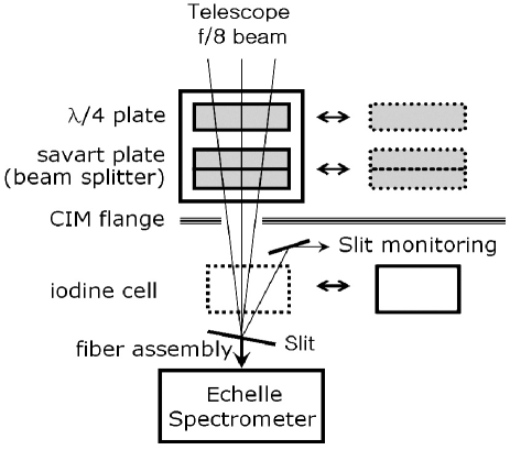
Figure 2: The optical layout of the polarimetric optics in front of the CIM of the 1.8-m telescope

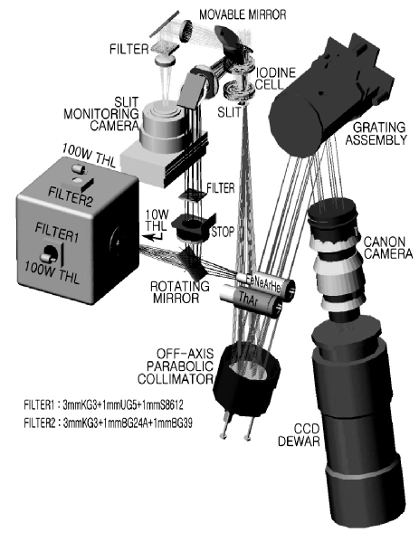
Figure 3: The optical layout of the BOES CIM. The long slit spectrograph, slit monitoring device and the calibration lamp unit can be seen at the right, left and front part respectively in this figure. Fiber input of the fiber assembly (omitted in this figure) is located at the slit position (see the Fig.2).

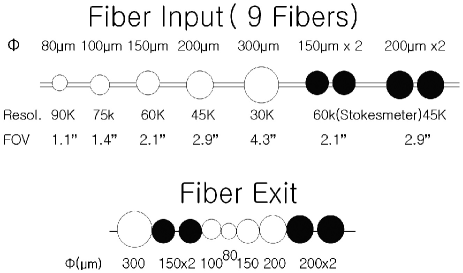
Figure 4: The scheme of the fiber input and exit in the BOES. Resolutions and fields of view are presented. The black circles denote the pairs of fiber for the spectropolarimeter.

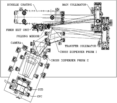
Figure 5: The spectrometer part of the BOES on the optical bench. The black anodized enclosure to block the dust and the turbulence from air circulation, and a baffle screen to block the stray light were omitted in this figure. CFC in this figure denotes Continuous Flow Cryostat dewar.

The block diagram of the BOES is presented in Fig. 1. The instrument consists of three main parts; 1) polarization optics (BOESP, Fig. 2) containing a rotatable quarter wave plate(QWP) and a Savart plate (SVTP) as a beam splitter, 2) CIM (Cassegrain Interface Module, Fig. 3) with a light transmitting fiber set (Fig. 4), and 3) a spectrometer (i.e. a bench mounted echelle spectrograph, Fig. 5). The 18.5 m length optical fibers transmit the star light accumulated at the Cassegrain focus to the spectrometer room where the temperature and humidity maintained to 20 $\pm$ 0.5 ^∘C and below 50 $\%$ respectively.

In addition to the high resolution echelle mode, BOES is equipped with a medium dispersion long slit spectrograph (called LS) in the CIM (Fig. 3). The LS can obtain a spectrum of a linear reciprocal dispersion of 19 to 217 $\AA$/mm (0.45 to 5.2 $\AA$/px) with 3.6 arcmin. slit length. The device switching between BOES (ordinary spectroscopic mode), BOESP (spectropolarimetric mode) and LS (long slit spectroscopic mode) can be done within 10 seconds.

As shown in Fig. 1, the BOES uses three CCDs : a slit monitoring CCD (called SMCCD), LS CCD and the BOES CCD. For the SMCCD, we use the Quantix 57 camera which has EEV 57-10 CCD chip (530 x 526, 13 $\mu$m pixel) with 2.7 arcmin. field of view. The LS CCD has Tek 1024 chip (1024 x 1024, 24 $\mu$ pixel) with the readout noise of 7.4 e^-. The BOES CCD is a grade zero class E2V CCD44-82 chip (2048 x 4096, 15 $\mu$m pixel) with 4.0 e^- readout noise.

Three personal computers (PC) are used to control the instrument. The PC $\sharp$1 connected to the CIM through RS232C controls the CIM. The observer can monitor the slit image and control the CIM by the PC $\sharp$2 connected to the PC $\sharp$1 by network. And the data acquisition from the BOES CCD or LS CCD is performed by a Linux based PC $\sharp$3.

2.1 Polarimetric optics

The polarimetric analyzer that we use in the spectropolarimetric mode consists of a rotatable QWP for polarimetric modulation, and Savart plate as a beam-splitter. In the present design we have decided to use the polymer QWP (Samoylov et al., 2004) instead frequently used Quartz/MgF₂ crystal wave plate or Fresnel rhombs. It is well-known fact, that the Quartz/MgF₂ QWP gives significant artificial polarization ripples of 0.05 to 2 $\%$ (Harris & Howarth (1996), Donati et al. (1999)) due to the interference within the cemented layers of the retarder. And well known solution based on Fresnel rhombs can not easily be used in our design due to the considerable size of these optics. In the same time, the used polimer QWP gives the wave retard of 0.25 $\pm$ 0.007$\lambda$ in 4000 $\sim$ 8000 $\AA$ range (Samoylov et al., 2004), and the ripple below 0.1 $\%$ (Ikeda et al., 2003). Such good parameters of the plate make it possible to use it alternatively. With these optical elements the available working wavelengths of the polarimeter is 4000 – 8000 $\AA$.

The optics are installed at the Cassegrian focus in front of the fiber input as shown in Fig. 2. It is mounted on rotary stages to be removable from the optical axis in case of ordinary spectral observations. The spectropolarimetric observations are available with resolving power of 45000 or 60000.

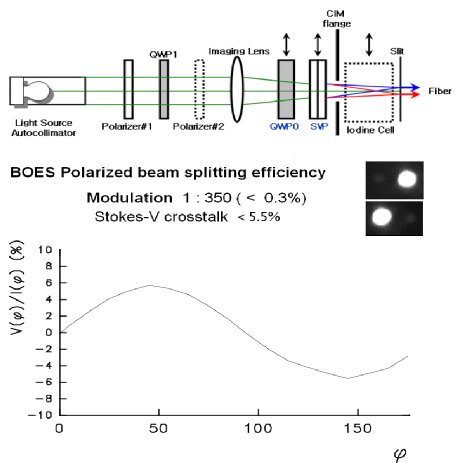
Figure 6: The optical layout of the modulation and crosstalk measurements (the upper plot), and the results of the crosstalk measurements (the lower plot). While measuring the crosstalk, the QWP#1 was removed.

Before each run of the polarimetric observations, the adjustment of the polarimeter is examined using a laboratory source of the light (for example, similar procedure is described in details by Plachinda (2005)). Some important examples of these tests are presented in Fig. 6, where the upper plot illustrates the analyzer assembled for measurements of the modulation by the QWP in observations of circular polarization. Artificial circularly polarized light is created by the combination of additional quarter-wave plate (QWP1) and polarizer (polarizer#1) as shown in the figure. The efficiency of the modulation is better than 99.7% . The lower plot (graph) illustrates the results of crosstalk measurements obtained at different orientation angles (the horizontal axis) of polarizer#1 (the QWP1 is removed in this case). As one can see, maximum crosstalk (vertical axis in the figure) which characterizes artificial circular polarization from linearly polarized light is not higher than 5.5% . To our knowledge, this result is practically standard for modern polarimeters.

2.2 The CIM and the fiber assembly

As the design concept of the CIM and the fiber assembly was described in Kim et al. (2002), we do not mention it here in details. Since then, we revised the flat-fielding lamps and the fiber assembly that was adopted for polarimetric observations. For the white balance of the flat fielding, we use three tungsten halogen lamps with an integration sphere – a 10 watts lamp with a half inch diameter aperture for the red wavelengths, a 100 watts with 1 inch diameter filters (3mmKG3 + 1mmBG24A + 1mmBG39) for the medium wavelengths, and a 100 watts with 2 inch diameter filters (3mmKG3 + 1mmUG5 + 1mmS8612) for the blue region (see the cube type integrating sphere in Fig. 3).

The BOES is furnished with nine fibers of 80, 100, 150, 200 and 300 $\mu$m in core diameters that provides corresponding spectral resolutions $\lambda$/$\Delta\lambda\sim$  90000, 75000, 60000, 45000 and 30000 respectively (Fig. 4). Five of them are used for ordinary spectroscopy, and two pairs of 150 and 200 $\mu$m fibers for spectropolarimetry. At the fiber input, fibers in each pair are separated by 500 $\mu$m distance that corresponds to the separation of the beams split by the polarimetric analyzer. At the fiber exit, these are separated to 380 $\mu$m to avoid overlapping of spectral orders. All the fibers except the 80 $\mu$m one (STU, Sch$\ddot{o}$tz et al. (1998)) are FBP (Polymicro Tech., 2004), transmission of which is improved relative to STU fiber, especially in the blue region.

2.3 Spectrometer part

The spectrometer (BOES) was designed by SSV and is shown in Figure  5. It is a quasi-Littrow configuration in the dual-white-pupil (DWP) configuration pioneered by UVES (Dekker et al., 1992) on the VLT. Other similar style DWP spectrometers are FOCES (Pfeiffer et al., 1998) of the 2.2-m telescope at Calar Alto Observatory, HRS (Tull, 1998) on the HET, and FEROS (Kaufer & Pasquini, 1998) at ESO.

In the BOES design, the f/8 beam exiting the fiber is collimated by the main off-axis collimator into a 136 mm diameter beam which is then dispersed by a 41.59 gr/mm R4 echelle of size 203 x 813 mm. This echelle is a replica of the master ruled for the blue side of UVES. The dispersed light from the echelle returns in quasi-Littrow mode (0.6^∘ out of plane) back to the main collimator and, via the folding mirror, to the transfer collimator. The transfer collimator is identical to the main collimator and the optical axes of both are co-linear. The transfer collimator corrects, to a high degree, the aberrations introduced by the main collimator and provides a white pupil near the cross-disperser to minimize the required clear apertures of the prisms and camera. Both collimators are cut from a common f/1.8 parent parabola of 600 mm diameter. All the mirrors have durable high-reflectance silver coatings.

Most if not all previous versions of DWP spectrometers incorporated a toroidal rear surface in the optical train (near the focal plane) to counteract astigmatism introduced by the quasi-Littrow white pupil collimation combination. However, we found that slightly pistoning the transfer collimator provides an equally viable solution that eliminates the need for this aspheric optic.

For the cross disperser, we adopted the use of a pair of 55^∘ prisms instead of a grating. Prisms provide more uniform order separation and higher efficiency across the very wide spectral bandpass of BOES. We used S-BSL7Y, a BK-7-like glass with enhanced ultraviolet transmission and available from Ohara, Inc. It was selected on the basis of its unusually high ratio of red to blue dispersion, creating a more uniform order separation across the echelle format, and thus more efficient order packing. The f/1.6 camera has an effective focal length of 389 mm and consists of six spherical lenses in 3 groups. It works over about a 9.5^∘ diameter field of view and spans the entire 3500 – 10,500 $\AA$ range with adequate image quality. All prisms and camera lenses were treated with wide-band anti-reflection coatings, which provide reflectance below 1.5$\%$ across the 3500 to 10,500 $\AA$ range. Overall, 86 spectral orders, from the 46th to the 131st, are captured on the CCD. Inter-order stray light appears to be less than 2$\%$ of the intensities of the neighboring orders.

2.4 Efficiency and stability of the BOES

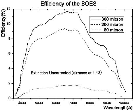
Figure 7: Measured efficiency of the (BOES + telescope + air extinction) for different single fibers without the correction of the light cutoff at the fiber input while the star at 1.13 airmass with the seeing around 2.3 arcseconds on 3rd Nov., 2003.

Fig. 7 illustrates the typical efficiency of the BOES measured on 3rd November 2003 with different (300, 200 and 80 $\mu$m in diameter) single fibers. This shows maximum efficiency is up to 12$\%$ including the light loss due to the atmospheric extinction, the reflectance of the telescope and the light cutoff at the fiber input. While measuring the efficiency, the target star was at the airmass of 1.13 with the seeing size around 2.3 arcseconds. The small efficiency of the 80 $\mu$m fiber comes from the light cutoff at the fiber input due to the small diameter (Kim et al., 2002).

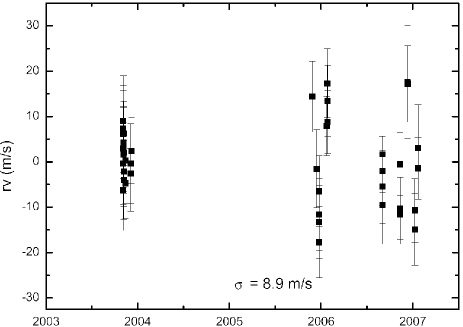
Figure 8: Radial velocity variation in Tau Ceti measured by the BOES for three years.

Good mechanical stability of the spectrograph makes it possible to use the instrument in a wide range of observational programs, for example, asteroseismology as well as Zeeman observations. Fig. 8 illustrates the typical accuracy of the stellar radial velocity measurements achieved in observations with the BOES equipped with an iodine cell. The standard star Tau Ceti (G8V) exhibits no any variations in radial velocities within typical accuracy about 9 m/s on three years time base.

3 Measurements of stellar magnetic fields with the BOES

3.1 Preliminary remarks

Directly, stellar magnetic fields are detected mainly through the observations of the Zeeman effect in spectral lines. According to basic physical principles (for more details see, for example, Landstreet (1980)) if an atom is placed in a magnetic field $B$, its individual energy levels are split into 2J + 1 sub-levels separated by energy $\Delta E=ge\hslash B/2mc$, where $g$ is the Lande factor. As a result, stellar magneto-sensitive spectral lines are split into a number of $\pi-$ and $\sigma-$ components which are polarized depending on the orientation of the magnetic field relative to the observer.

In a longitudinal (parallel to the line of sight) magnetic field the $\sigma-$ components, which are generally displaced symmetrically to shorter and longer wavelengths relative to the non-shifted central $\pi-$ components of spectral lines, have opposite circular polarizations. Thus by observing circular polarization in the spectral lines we are able to measure the longitudinal component of stellar magnetic field. To reconstruct full vector of the field, additional observations of linearly polarized $\pi-$ and $\sigma-$ components are needed. These observations allow to estimate a transverse field component that together with observations of the longitudinal component give full vector magnetic field averaged over the stellar disc. In this paper, we discuss observations of the longitudinal fields only.

The averaged circularly polarized $\sigma-$ components are displaced relative to the rest wavelength $\lambda_{0}$ of a spectral line by a factor of

$$\Delta\lambda_{B}=\pm 4.67\times 10^{-13}z\lambda^{2}B_{l},$$ (1)

where $B_{l}$ is the longitudinal field component in gauss, $z$ is the effective Lande factor, $\lambda$ is the wavelength in $\AA$. Due to the fact that these displaced components have opposite circular polarizations and are shifted relative to each other, in the stellar circular polarization spectra (Stokes-V spectra, or V spectra) they form non-zero features within magneto-sensitive spectral lines. In most cases of spectropolarimetric observations these features show well-known S-shaped features (Fig. 9) at the cores of spectral lines. Their amplitudes and forms depend on magnetic field strengths, Lande factors, gradients of the line profiles and spectral resolution of a spectrograph:

$$V\sim zB_{l}(dI/d\lambda)$$ (2)

where $dI/d\lambda$ describes the gradient of a spectral line convolved with instrumental function of a spectrograph (Landstreet, 2001, for instance). The mean longitudinal magnetic field can be estimated by applying model methods of Doppler-Zeeman spectropolarimetric tomography to the analysis of the Stokes-V spectra (Euchner et al., 2002, for instance), or the LSD method (Donati et al., 1997). Alternatively (and traditionally) longitudinal magnetic fields can simply be measured via analysis of the displacement (1) between the positions of spectral lines in the spectra of opposite circular polarizations split by analyzer.

3.2 Obtaining circular polarization spectra: observations and data reduction

Each exposure in inobservations of circular polarization with the BOES yields two spectra on the CCD – one from the ordinary beam and the other from the extraordinary beam split by the analyzer. In case of an ideal spectropolarimeter (which has no any intrinsic distortion factors), this single exposure obtained at one of the orthogonal orientations of the quarter-wave plate would practically be enough to build V-Stokes spectra and to measure the magnetic field. However, due to the presence of a large number of instrumental biases such as pixel-to-pixel inhomogeneity, slightly different dispersion relationships at each of the split beams and other factors, it is recommended to obtain an additional exposure with inverted sign of the polarization effects by rotating the quarter-wave plate by $90^{\circ}$. Such a technique makes it possible to reconstruct the Stokes-V spectra in pixel coordinate system separately for the spectra of the ordinary and extraordinary beams that significantly increases the quality of the output results (for details see, for instance, Plachinda & Tarasova (1999), Bagnulo et al. (2002) or Aznar Cuadrado et al. (2004)).

Due to the above mentioned reasons and in order to increase reliability of our observations of circular polarization, one observation with the BOES consists of four short, consecutive exposures at two orthogonal orientations of the quarter-wave plate (the sequence of its position angles is $+45^{\circ},-45^{\circ},-45^{\circ},+45^{\circ}$). Assuming a priori that the time-scale of possible physical variability of polarization features in spectra of non-degenerate stars would be as short as a few hours, we usually set the integration time for each of the individual exposures from a few minutes to 0.5 hours depending on stellar magnitude and sky conditions.

The data reduction was processed with IRAF. The procedures are mostly standard including the following steps: cosmic ray hits removal, electronic bias substraction, flat-fielding, 2-D wavelength calibration, sky background substraction, spectrum extraction. As an output result we obtained a series of pairs of left and right circular polarized spectra that we used to build V-Stokes spectra and measure stellar longitudinal magnetic fields. We obtained the individual $Stokes-V$ spectra for each of the echelle spectral orders by applying the technique presented by Bagnulo et al. (2002).

In order to illustrate results of the reduction in our first polarimetric observations with the BOES, we present fragments of circular polarization spectra of the magnetic stars HD215441, HD32633, HD40312 and the star HD61421 (Procyon) in Figs. 9,10. We have chosen these stars as the remarkable cases of typical magnetic stars (HD215441, HD32633, HD40312) having polarization features of different intensities (details on these stars are also presented below) and zero-field (Procyon) star. As one can see (Fig. 9), the circular polarization of different intensities can easily be resolved and studied with our polarimeter.

Examination of the zero-field star Procyon has revealed no any artificial circular polarization features at a characteristic level of about 0.5% within the working wavelength region from 4000Å  to 8000Å. The lower plot in Fig. 9 demonstrates zero polarization of Procyon at the H$\beta$ region. An example of another wavelength region is presented in Fig. 10.

3.3 Linear polarization

Finally, before presentation of the results of the longitudinal magnetic field measurements in the standard stars, we would also like briefly discuss the possibility to obtain $Stokes-Q/U$ (linear polarization) spectra that is necessary for measurements of the transverse magnetic fields. It should be noted, that linear polarization features in spectral lines due to Zeeman effect are intrinsically weaker than the corresponding circular polarization features. This strongly complicates observations of linear polarization with 2-m class telescopes. To simplify the solution, special methods of data reduction (Donati et al., 1997) and the LSD method for obtaining averaged per all spectral lines linear polarization (Donati et al., 1997) should be applied. In this paper we do not discuss these details addressing them for further special consideration of the problem in application to the BOES. Here we just briefly present and illustrate test observations of the $Stokes-Q/U$ spectra with the BOES.

There are several designs of polarimetric optics for obtaining all $Stokes$ parameters including $Stokes-Q/U$. Due to technical limitations, for linear polarization measurements we have chosen simplest configuration of polarimetric optics similar to that presented by Naydenov et al. (2002). According to their scheme, the $Stokes-Q/U$ spectra can simply be obtained by using the beam splitter only (without the QWP). In this case, the necessary observational basis is achieved by rotation of the cassegrain assembly with obtaining of four consecutive exposures at different position angles of the beam splitter relative to the sky plane (for details see Naydenov et al. (2002)). Applying this method, we observed the magnetic star $\alpha^{2}$ CVn which shows rotationally modulated linear polarization in spectral lines of its spectrum.

According to Wade et al. (2000), net linear polarization of this star varies from about -0.2% to about +0.6% . We observed $\alpha^{2}$ CVn at two phases of the star’s rotation when the polarization is nearly zero ($\phi\approx 0.03$) and at one of the extrama ($\phi\approx 0.2$) where the star’s spectrum exhibits non-zero positive linear polarization ($Stokes-Q\approx+0.6$% and $Stokes-U\approx+0.3$% , see Fig. 6 in Wade et al. (2000)). Such a weak polarization level can not simply be registered within consideration of one individual spectral line. However, the problem can be resolved if several spectral lines are considered together. Say, considering net polarization as a function of the distance from the line cores (in the radial velocity scale), the LSD method of obtaining averaged per all available spectral lines polarization can be applied (Wade et al., 2000). To illustrate this, in Fig. 11 we present averaged per all available Balmer lines $Stokes-Q/U$ spectra of $\alpha^{2}$ CVn. The left two plots illustrate zero polarization at the rotation phase $\phi\approx 0.03$. The right plots present nearly maximum positive polarization at the rotation phase $\phi\approx 0.2$. Signatures of the narrow, about 0.6% polarization features are clearly seen at the line cores in this case. As one can see, even such weak polarization level can also be registered with our polarimeter that enables us to measure the transverse magnetic field. This problem, however, deserves additional special paper where we will present all the necessary tool for these measurements and details on linear polarization observations of the standard stars including $\alpha^{2}$ CVn that we briefly touched here. In this paper we limit ourself with presentation of the polarimeter and consideration of the longitudinal magnetic field measurements only.

3.4 Measurements of stellar longitudinal magnetic fields with the BOES

In our first Zeeman observations of stellar magnetic fields with the BOES we measured longitudinal fields via analysis of the displacement (Equation 1) between the positions of spectral lines in the spectra of opposite circular polarizations (see, for instance, Monin et al. (2002) and references therein). This technique, if applied to all selected spectral lines in a spectrum with further statistical averaging of the result, is quite robust for the determination of longitudinal magnetic fields averaged over the stellar disks. The atomic data necessary for the identification of spectral lines and their Lande factors were taken from the VALD database (Piskunov et al., 1995; Ryabchikova et al., 1999; Kupka et al., 1999).

Measurements at individual spectral lines were carried out in pixel coordinate system separately for spectra obtained at the ordinary and extraordinary beams split by the analyzer to avoid uncertainties in the wavelength calibration. In this case, Zeeman displacement between $\sigma$ components of opposite circular polarizations can be measured as a shift between the centers of gravity of a spectral line extracted from the same pixels of two neighboring CCD frames obtained at two orthogonal orientations ($+45^{\circ}$ and $-45^{\circ}$) of the quarter-wave plate. The longitudinal magnetic field $B_{l}$ based on these measurements can be found as an averaged mean of $B_{l}^{o}$ and $B_{l}^{e}$ estimates of the magnetic field obtained from spectra of the corresponding ordinary and extraordinary beams. It is clear, that $B_{l}^{o}$ and $B_{l}^{e}$ are not free of any biases due to the influence of mechanical instabilities from an exposure to exposure. Their averaging, however, significantly reduces them as we now illustrate.

Denoting the center of gravity of spectral lines from the ordinary/extraordinary spectrum obtained at $+45^{\circ}$ or $-45^{\circ}$ position of the quarter-wave plate as $\lambda^{o}_{+45^{\circ}}/\lambda^{e}_{+45^{\circ}}$ or $\lambda^{o}_{-45^{\circ}}/\lambda^{e}_{-45^{\circ}}$, the $B_{l}^{o}$ and $B_{l}^{e}$ estimations have the following forms:

$$B_{l}^{o}=\pm k(\lambda^{o}_{+45^{\circ}}-\lambda^{o}_{-45^{\circ}})/2=k(\pm 2\Delta\lambda_{B}\pm\Delta\lambda_{o})/2$$ (3)

$$B_{l}^{e}=\mp(\lambda^{e}_{+45^{\circ}}-\lambda^{e}_{-45^{\circ}})/2=k(\pm 2\Delta\lambda_{B}\mp\Delta\lambda_{e})/2$$ (4)

where $k=1/(4.67\times 10^{-13}z\lambda^{2})$; $\Delta\lambda_{B}$ is Zeeman displacement between the $\sigma$ components in the spectral line; $\Delta\lambda_{o}$ and $\Delta\lambda_{e}$ are instrumental shifts between spectra of the ordinary/extraordinary beam obtained at different time moments due to the requirement to have two consecutive exposures at $+45^{\circ}$ and $-45^{\circ}$ orientations of the quarter-wave plate. The sign inversion in $B_{l}^{e}$ estimation appears due to the inverse polarimetric properties of the extraordinary beam relative to the ordinary one. Averaging the data we have:

$$B_{l}=B_{l}^{o}/2+B_{l}^{e}/2=k(\pm 4\Delta\lambda_{B}\pm\Delta\lambda_{o}\mp\Delta\lambda_{e})/4.$$ (5)

In eq.(5), the instrumental shift is taken with opposite sign due to the polarimetric inversion in the beams. Practically in all cases of any instrumental effect these shifts are equal in linear guess approximation and eliminated each other in the applied method.

Obtaining an estimate of the averaged mean longitudinal magnetic fields and error bars within one observation of a star (consisting of four consecutive exposures) was done by weighting and statistically averaging all the individual measurements. Here, we weighted individual line-by-line measurements by residual intensities and signal-to-noise ratios as described by Monin et al. (2002). Alternatively, we also applied the Monte-Carlo simulation method (Plachinda, 2004a) of obtaining error bars and weights for the individual measurements.

4 Results of Zeeman observations of standard stars

The observations were carried out in the course of one observing night on 27th September, 2006. Three well known magnetic Ap/Bp stars HD215441, HD32633 and HD40312 ($\theta Aur$) were observed together with Procyon as a zero-field standard. Table 1 gives an overview of the observations.

Results of the longitudinal magnetic field measurements are summarized in Table 2, where column 1 is the name of a star, column 2 is the spectral class, column 3 is the visual magnitude, column 4 is the exposure time, column 5 is the rotational phase of a magnetic star if known (throughout this study we use ephemeris presented by Wade et al. (2000)), columns 6-7 report the measurements and uncertainties of the longitudinal magnetic fields obtained as explained above. We briefly discuss these results.

HD215441 or the famous Babcock’s star is known to have the strongest magnetic field among the main sequence stars. The longitudinal field of this star varies with the rotational period P = 9.4871 days about the mean value of $+15000$ G with an amplitude of about 4.5 kG (Bychkov et al., 2005). Our result($B_{l}=+10500\pm 330$ G, see Table 2), which is consistent with the data presented by Bychkov et al. (2005), was measured as the average mean of individual Zeeman measurements obtained from all available 68 spectral lines (including hydrogen lines) in the region between 4100Å  and 8000Å . Unfortunately, due to uncertainties in determination of the magnetic ephemeris of this star (Bychkov et al., 2005) we are unable to compare our result with other authors’ ones. Besides, measurements of $B_{l}$ by using only metal lines compared to measurements by hydrogen lines exhibit a very large discrepancy (much larger than corresponding scatter due to Poisson noise), that suggests the presence of a very complicated magnetic field morphology in this star. For example, measurements of the magnetic field by using only the Balmer lines gives $B_{l}=+17000\pm 700$ G that is confidentially larger than the field averaged by individual measurements of all the other spectral lines. In this study we do not discuss this well-known effect (Bychkov et al., 2005, and references therein) presenting HD215441 only as an illustration.

HD32633 and HD40312 or $\theta Aur$ are well-known broad-lined B9p and A0p magnetic stars which we used as standards to compare our measurements with the best measurements given by other authors. To our knowledge, the most extensive high-precision measurements of their variable magnetic fields were performed by Wade et al. (2000).

According to Wade et al. (2000), the longitudinal magnetic field of HD32633 varies with the period of 6.4300 days and demonstrates smooth, non-sinusoidal variation with two extremes at $B_{l}\approx-4200$ G and $B_{l}\approx+1800$ G. Our single observation of this star was carried out at the rotation phase $\phi=0.012$ under the moderate weather conditions. At this phase the longitudinal magnetic field of this star is located at arising branch of the field variation between the negative extremum and crossover. With our polarimeter, the measured longitudinal field at this phase ($B_{l}=-2616\pm 56$ G, see Table 2) have demonstrated a very good agreement with results of other authors. In Fig. 12 (the lower plot) our observation (filled triangles) is illustrated in comparison with the data (open circles) taken from Wade et al. (2000). The obtained field value and small error bar (in Fig. 12 the error bar is smaller than the triangle size) suggest high quality of our polarimeter in measurements of stellar magnetic fields. In particular, the previous best estimations of the mean longitudinal magnetic field of this star demonstrated the same or twice lower accuracy (Wade et al., 2000).

The star HD40312 exhibits weak variable longitudinal magnetic field the behavior of which is presently well-studied (Wade et al., 2000). Our observations of HD40312 were carried out under poor weather condition that made us observe this star for a quite long time (about one hour, Table 1). We have observed this target at the rotation phase $\phi\approx 0.6$ of the field variation. Similar to the previous star, our estimation of the field is well consistent with results given by Wade et al. (2000) (see Table 2 and the upper plot in Fig. 12).

HD61421 (or $\alpha$ CMi, Procyon) was finally used as a zero-field star. This star was observed polarimetrically by a number of authors (see an overview in Table 3). In their observations magnetic field has not been found with typical accuracies from about 1 G to 7 G. Formal averaging of these results gives no any traces of magnetic field at a level of about 0.5 G that makes us possible to use this star as a well-studied zero-field standard. Our result also showed a very accurate zero with error bar of about 2 G (see Table 2). This result has been obtained during just about 6 min of integration in contrast to hours of typical exposure times in the previous observations of this star (see Table 3). About one hundred non-blended spectral lines were used to obtain this result.

It should be noted here that such a high accuracy of the field measurement becomes critical to the adopted methods of data reduction and the measurements. In our measurements, for example, different methods of statistical analysis in the applied line-by-line technique gave us some differences in the final result. Obtaining statistical weights of the measurements at individual spectral lines using their residual intensities and signal-to-noise ratios, we initially derived the uncertainty of about 2.7 G. However, from the measurements weighted by Monte-Carlo simulation method (Plachinda, 2004a), the final error bar was determined with significantly better accuracy of about 2.2 G. This fact can easily be understood because there are more than the above mentioned two factors (poisson noise and residual intensities) influence to the statistical weights. The Lande factors (their values) and shapes of spectral lines also play roles. The applied Monte-Carlo method takes them all into account.

At the same time, methods of weighting do not play such a significant role in the determination of strong mean longitudinal fields in chemically peculiar magnetic stars. In these stars the main contribution to the uncertainty comes from the inhomogeneous distribution of the magnetic field over the surface and chemical peculiarities that may demonstrate local field intensities at chemically overabundant spots (such as in our example with HD215441).

Different methods of the data reduction also play a role (extraction of spectral orders, for example). In this paper, however, traditional standard methods were adopted for the spectropolarimetric analysis to demonstrate the pilot workability of the BOES spectropolarimeter.

5 Summary

We have presented the new stationary spectropolarimeter mounted on the high-resolution fiber-fed echelle spectrograph BOES of the 1.8-m telescope at the BOAO. At the moment the instrument is ready for regular observations of stellar longitudinal magnetic fields and demonstrates good transparency and precision of the measurements. Typical accuracies of the field measurements in bright stars (brighter than 9th stellar magnitude) range from about 2 to a few tens of gauss depending on spectral class, rotation of a star and integration time. In this part, further improvements to the polarimeter concern mainly the software for the data reduction and methods of the measurements. We expect, that applying more advanced technologies of the data reduction connected, for example, with optimal extraction of spectral orders (Donati et al., 1997) or the LSD method for measurements of weak magnetic fields (Donati et al., 1997), the instrument will demonstrate even better results. Further examination of these points will be among the goals of our final study upon final upgrade of the polarimeter.

Table 1: Journal of observations. The first column gives name of an observed star, the second column lists the Julian date (JD) of the midpoint of the observation, the third and fourth columns are total exposure time Exp and corresponding number of observations N_obs, fifth and sixth columns are total signal to noise ratio S/N at $\lambda 5500$ and weather conditions (WC: good/moderate/poor).

Name	JD	Exp (sec)	Nobs	S/N	WC
HD32633	2454006.065278	8400	1	350	moderate
HD40312	2454006.256944	3840	3	400	poor
HD61421	2454006.333333	395	1	600	poor
HD215441	2454005.981944	7200	1	180	moderate

Table 2: Determination of the mean longitudinal field.

Name	SP	mv	Exp (sec)	$\phi$	Bl (G)	$\sigma$ (G)
HD32633	B9p	7.1	8400	0.13	-2616	56
HD40312	A0p	2.6	3840	0.61	+310	28
HD61421	F5	0.34	395	–	-3.8	2.2
HD215441	B9p	8.8	7200	–	+10500	330

Table 3: An overview of the mean longitudinal magnetic field observations of $\alpha$ CMi.

Author	Aperture	Polarimeter	$Exposure$	$B_{e}$	$\sigma$
	(meters)		(hours)	(G)	(G)
Landstreet (1982)	2.6	magnetometer	?	7	7
Borra et al. (1984)	2.5	multislit magnetometer	?	-7.5	5.9
Glagolevsky et al. (1991)	6.0	magnetometer	?	17	7.1
Bedford et al. (1995)	1.9	triple magnetooptical	8	-1.86	0.9
		filter with a potassium cell		0.49	0.8
Plachinda & Tarasova (1999)	2.6	stokesmeter + CCD	2.2	-1.34	1.0
Shorlin et al. (2002)	2.0	stokesmeter + CCD	?	2.0	5.0

Figure 9: Stokes $V$ spectra (from top to bottom) of the stars HD215441, HD32633, HD40312 and the star HD61421 (Procyon) in at the H$\beta$ line region.

Figure 10: Another fragment of Stokes $I$ and $V$ spectra of Procyon around $\lambda 5500$. There are no any signatures of artificial circular polarization features in all the studied wavelength region.

Figure 11: Averaged per basic Balmer lines Stokes $Q/U$ parameters of the star $\alpha^{2}$ CVn at those rotational phases where the star exhibits zero ($\phi\approx 0$, left plots) and maximun ($\phi\approx 0.2$, right plots) linear polarization. The data are presented in the radial velocity scale as functions of the distance from the spectral line cores.

Figure 12: Comparison of our Zeeman observations of longitudinal magnetic fields of the stars HD40312 and HD32633 (filled triangles) with observations of Wade et al. (2000) (open circles).

References

- Appenzeller et al. (1998) Appenzeller, I., Fricke, K., Furtig, W., et al., 1998, The Messenger, 94, 1.
- Aznar Cuadrado et al. (2004) Aznar Cuadrado, R., Jordan, S., Napiwotzki, R., Schmid, H.M., Solanki, S.K., & Mathys, G. 2004, A&A, 423, 1081
- Bagnulo et al. (2002) Bagnulo, S., Szeifert, T., Wade, G.A., Landstreet, J.D., & Mathys, G. 2002, A&A, 389, 191
- Bailey (1989) Bailey, J. 1989, in Spectropolarimetry at the AAT (The AAT User’s Manual No. 24)
- Bedford et al. (1995) Bedford, D.K., Chaplin, W.J., Davies, A.R., Innis, J.L., Isaak, G.R., and Speake, C.C., 1995, A&A, 293, 377
- Borra et al. (1984) Borra, E.F., Edwards, G., and Mayor, M., 1984, ApJ, 284, 211
- Bychkov et al. (2005) Bychkov, V.D., Bychkova, L.V., & Madej, J. 2005, A&A, 430, 1143
- Dekker et al. (1992) Dekker, H., Delabre, B., Hess, G., Kotzlowski, H., 1992, ”Progress in Telescope and Instrumentation Technologies”, ESO Conference and Workshop Proceedings, ESO, edited by Marie-Helene Ulrich, p. 581
- Donati et al. (1997) Donati, J.-F., Semel, M., Carter, B.D., Rees, D.E., & Cameron, A. 1997, MNRAS, 291, 658
- Donati et al. (1999) Donati, J.-F., Catala, C., Wade, G.A., Gallou, G., Delaigue, G., Rabou, P., 1999, A&AS, 134, 149
- Donati et al. (2003) Donati J.-F., Cameron A. Collier, Semel M., Hussain G. A. J., Petit P., Carter B.D., Marsden S.C., Mengel M., Lopez Ariste A., Jeffers S.V., Rees D.E. 2003, MNRAS, 345, 1145
- Eversberg et al. (1998) Eversberg, T., Moffat, A.F.J., Debruyne, M., Rice, J.B., Piskunov, N., Bastein, P., Wehlay, W.H., & Chesneau, O. 1998, PASP, 110, 1356
- Euchner et al. (2002) Euchner, F., Jordan, S., Beuermann, K., Gänsicke, B.T., and Hessman, F.V., 2002, A&A, 390, 633
- Glagolevsky et al. (1991) Glagolevsky, V., Romaniuk, I., Naidenov, V.G., Shtol, V.G., 1991, Bull. Spe. Astrophys. Obs., North. Caucasus, 27, 32
- Goodrich et al. (1995) Goodrich, R.W., Cohen, M.H., & Putney, A. 1995, PASP, 107, 179
- Harris & Howarth (1996) Harris, T.J., and Howarth, I.D. 1996, A& A, 310, 533
- Hubrig et al. (2006) Hubrig, S., Briquet, M., Schller, M., De Cat, P., Mathys, G., & Aert, C., 2006, MNRAS, 369, L61
- Ikeda et al. (2003) Ikeda, Y., Akitaya, H., Matsuda, K., Kawabata, K. S., Seki, M., Hirata, R., Okazaki, A., 2003, SPIE Proc., 4843, 437
- Kaufer & Pasquini (1998) Kaufer, A., Pasquini, L., 1998, SPIE Proceedings ”Optical Astronomical Instrumentation”, ed. by S. D’Odorico, S. vol.3355, p. 844
- Kim et al. (2002) Kim, K. M., Jang, B. -H., Han, I., Jang, J. G., Sung, H. C., Chun, M. Y., Hyung, S., Yoon, T.-S., Vogt, S. S., 2002, Journ. of Korean Astron. Soc., 35, 221
- Kotov et al. (1998) Kotov V.A., Scherrer P.H., Howard R.F., & Haneychuk V.I. 1998, ApJS, 116, 103
- Kupka et al. (1999) Kupka F., Piskunov N.E., Ryabchikova T.A., Stempels H.C., & Weiss W.W. 1999, A&AS, 138, 119
- Landstreet (1980) Landstreet, J.D., 1980, AJ, 85, 611
- Landstreet (1982) Landstreet, J.D., 1982, ApJ, 258, 639
- Landstreet (2001) Landstreet, J. D. 2001, In: Magnetic Fields Across the Hertzsprung-Russell Diagram, G. Mathys, S.K. Solanki and D.T. Wickramasinghe (eds.), ASP Conf. Ser., 248, 277
- Manset & Donati (2003) Manset Nadine, & Donati, J.-F. 2003, Polarimetry in Astronomy. Edited by Silvano Fineschi. Proceedings of the SPIE, 4843, 425
- Monin et al. (2002) Monin, D.N., Fabrika, S.N., & Valyavin, G.G., 2002, A& A, 396, 131
- Naydenov et al. (2002) Naydenov, I.D., Valyavin, G.G., Fabrika, S.N., et al 2002, Bull. Spec. Astrophys. Obs., 53, 124
- Petit et al. (2005) Petit P., Donati J.-F., Auriere M., Landstreet J.D., Lignieres F., Marsden S., Mouillet D., Paletou F., Toque, N., & Wade G.A. 2005, MNRAS, 361, 837
- Pfeiffer et al. (1998) Pfeiffer, M. J., Frank, C., Baumuller, D., Fuhrmann, K., Gehren, T. 1998, Astron. Astrophys. Suppl. Ser. 130, 381.
- Piskunov et al. (1995) Piskunov N.E., Kupka F., Ryabchikova T.A., Weiss W.W., & Jeffery C.S. 1995, A&AS, 112, 525
- Plachinda (2004a) Plachinda S.I. 2004a, NATO Science Series, 161, 351
- Plachinda (2004b) Plachinda S.I. 2004b, In: ”Multi-Wavelength Investigations of Solar Activity” IAU Symposium No. 223, 689