Analysis of two-dimensional high-energy photoelectron momentum distributions in single ionization of atoms by intense laser pulses

Abstract

We analyzed the two-dimensional (2D) electron momentum distributions of high-energy photoelectrons of atoms in an intense laser field using the second-order strong field approximation (SFA2). The SFA2 accounts for the rescattering of the returning electron with the target ion to first order and its validity is established by comparing with results obtained by solving the time-dependent Schrödinger equation (TDSE) for short pulses. By analyzing the SFA2 theory, we confirmed that the yield along the back rescattered ridge (BRR) in the 2D momentum spectra can be interpreted as due to the elastic scattering in the backward directions by the returning electron wave packet. The characteristics of the extracted electron wave packets for different laser parameters are analyzed, including their dependence on the laser intensity and pulse duration. For long pulses we also studied the wave packets from the first and the later returns.

I Introduction

Much of our knowledge of strong field, multiphoton ionization processes comes from the study of above-threshold ionization (ATI). In this process an atom absorbs more photons than the minimum number required for the ejection of an electron. By measuring the energy of the photoelectrons, the characteristic ATI spectra are peaks separated by the photon energy, with the peak positions shifted by the ponderomotive potential. For long pulses, additional substructures due to Freeman resonances Freeman appear. For shorter pulses, of durations of the order of 10-20 fs or less, calculations have shown that the major ATI peaks are accompanied by subpeaks which have been attributed to the rapidly changing ponderomotive potential marlene1 ; bardsley .

Experimentally more information on ATI electrons can be determined by measuring the angular distributions or the 2D momentum distributions. For example, the nature of Freeman resonances are associated with individual Rydberg states by the number of lobes in their angular distributions helm03 . For short pulses in the tunneling ionization regime, recent experiments ullrich ; cocke have shown ubiquitous fan-like structures in the 2D momentum spectra for low-energy electrons. These fan-like structures are now also well-understood and they are due to the long-range Coulomb interaction between the tunnel ionized electron and the target ion it has left behind chen06 ; Arbo . These fan-like structures do survive the integration over the laser focus volume, as shown in recent comparison between theoretical calculations with experiments toru .

High-energy photoelectrons have been measured previously for atomic targets, both in energy and angular distributions, using longer pulses at lower intensities. The energy spectra above $4U_{p}$, where $U_{p}$ is the ponderomotive energy, have been found to vary rapidly with small changes in laser intensities hertlein ; paulus01 when laser pulse durations are larger than 20 to 30 fs. Different theoretical models have been used to interpret these phenomena, but the conclusions are still tentative so far muller ; maquet ; becker ; tony . While single ionization of an atom in an intense laser field has been calculated accurately by solving the time-dependent Schrödinger equation (TDSE) directly in the past two decades, the photoelectrons in the high-energy region, especially their momentum distributions, have not been investigated. This is not surprising since the photoelectron yield drops rapidly with the electron’s energy. On the other hand, it is known that rescattering plays a major role in many laser-atom interaction phenomena, including the generation of high-energy ATI electrons. Understanding the nature of these high-energy photoelectrons, especially their 2D momentum distributions, may help to shed new light on the rescattering process itself.

Recently we have initiated a careful study on the 2D momentum distributions of high-energy photoelectrons by directly solving the TDSE of a one-electron atom in a short laser pulse. By focusing on photoelectrons that have been backscattered we have been able to extract the elastic scattering cross sections by free electrons from the calculated laser-generated photoelectron spectra. For molecular targets this has the important significance that it offers the possibility of using infrared lasers for dynamic chemical imaging with temporal resolution of a few femtoseconds torunew . For short laser pulses, by studying the dependence of the 2D momentum spectra on the carrier-envelope phase, it also offers the possibility of directly characterizing the electric fields of few-cycle pulses.

To obtain 2D momentum electron spectra accurately in the high-energy region, say, up to about 10 $U_{p}$, calculations have to be done very carefully. For pulses as short as a few femtoseconds and intensities with Keldysh parameters $\gamma$ Keldysh close to one, we have been able to obtain accurate 2D momentum spectra from solving TDSE directly. Here $\gamma=\sqrt{I_{p}/(2U_{p})}$, with $I_{p}$ the binding energy of the electron, and $U_{p}=I_{\text{m}ax}/(4\omega^{2})$, where $I_{\text{m}ax}$ is the peak intensity and $\omega$ is the carrier frequency, of the laser, respectively. (Atomic units are used throughout unless indicated otherwise.) To extend such TDSE calculations to high laser intensities or long durations is computationally more challenging. We thus seek to examine the predictions based on the second-order strong-field approximation (SFA2) lew2 ; milosevic03OP ; milosevic03PRA ; milosevic04PRA ; milosevic05 ; faiser where the rescattering of the returning electron with the target ion is included. To establish the validity of SFA2, we first compare its results with those from solving the TDSE for short pulses. The SFA2 is then used to analyze high-energy photoelectron momentum distributions for various laser parameters. From such analysis, we show that electrons on the so-called back rescattered ridge (BRR) can be identified. The electron yield along the BRR can be used to extract elastic scattering cross sections of free electrons by target ions, as well as the wave packet of the returning electrons. Using SFA2 allows us to analyze the electron wave packets for longer pulses and higher intensities.

In the next Section we first summarize the first- and second-order amplitudes of the strong field approximation. The results from using this theory for the prediction of the 2D momentum spectra are shown in Section III. The conclusion is given in Section IV.

II Theoretical models

To study atoms in an intense laser field, there are only two general theoretical tools at present. One is to numerically integrate the TDSE and the other is based on the SFA. Both approaches have their limitations. For TDSE, to obtain high precision in small quantities such as the momentum distributions of high-energy electrons poses a computational challenge. This challenge is less severe for short pulses where the electron is confined to a smaller box such that accurate solution of the TDSE is possible. For longer pulses and higher intensities, high accuracy becomes harder to achieve. One has to check carefully the possible effect of reflection from the box boundaries as well as the convergence of the basis set used. While reflection can be avoided by matching the solution inside the box to the outside region where it is expanded in terms of Volkov states tong , such an approach requires large basis set in both the inside and the outside regions, and thus the method is also very computationally intensive. Thus in the TDSE calculations we limit ourselves only to short pulses. The numerical method we used for solving TDSE has been presented in our previous works chen06 ; toru . In this paper we only present the details of the SFA2 used here.

An exact expression for the probability amplitude of detecting an ATI electron with momentum p can be written formally as

$$f({\textbf{p}})=-i\lim_{t\rightarrow\infty}\int_{-t}^{t}dt^{\prime}\left\langle\Psi_{\textbf{p}}(t)\left|U(t,t^{\prime})H_{i}(t^{\prime})\right|\Psi_{0}(t^{\prime})\right\rangle.$$ (1)

Here $U(t,t^{\prime})$ is the time-evolution operator of the complete Hamiltonian

$$H(t)=H_{a}+H_{i}(t)$$ (2)

where

$$H_{a}=-\frac{1}{2}\nabla^{2}+V(\textbf{r})$$ (3)

is the atomic Hamiltonian, and

$$H_{i}(t)=\textbf{r}\cdot\textbf{E}(t)$$ (4)

is the laser-electron interaction in the length gauge and the dipole approximation. The linearly polarized electric field $\textbf{E}(t)$ of the laser pulse along the $z$ axis is given by

$$\textbf{E}(t)=E_{0}a(t)\cos(\omega t+\phi)\hat{z}$$ (5)

where $\phi$ is the carrier-envelope phase. The envelope function $a(t)$ is chosen to be

$$a(t)=\cos^{2}\left(\frac{\pi t}{T}\right)$$ (6)

for the time interval ($-T/2,T/2$), and zero elsewhere. In this paper, $T$ is defined as the (full) duration of the laser pulse which is 2.75 times of the FWHM (full width at half maximum) and the carrier-envelope phase $\phi$ is set as zero. The functions $\Psi_{\textbf{p}}(t)$ and $\Psi_{0}(t)$ are scattering state with asymptotic momentum p and the ground state, respectively, of the atomic Hamiltonian $H_{a}$. The time-evolution operator $U(t,t^{\prime})$ satisfies the Dyson equation

$$U(t,t^{\prime})=U_{\text{F}}(t,t^{\prime})-i\int_{t^{\prime}}^{t}dt^{\prime\prime}U_{\text{F}}(t,t^{\prime\prime})VU(t^{\prime\prime},t^{\prime})$$ (7)

where $U_{\text{F}}(t,t^{\prime})$ is the time-evolution operator for the Hamiltonian of a free electron in the laser field, which is

$$H_{\text{F}}=-\frac{1}{2}\nabla^{2}+\textbf{r}\cdot\textbf{E}.$$ (8)

The eigenstates of $H_{\text{F}}(t)$ are the Volkov states

$$\left|\chi_{\textbf{p}}(t)\right\rangle=\left|\textbf{p}+\textbf{A}(t)\right\rangle\exp[-iS_{\textbf{p}}(t)]$$ (9)

with the action

$$S_{\textbf{p}}(t)=\frac{1}{2}\int_{-\infty}^{t}dt^{\prime}\left[\textbf{p}+\textbf{A}^{\prime}(t)\right]^{2}.$$ (10)

The vector potential of the laser field $\textbf{E}(t)$ is denoted by $\textbf{A}(t)$, and $\left|\textbf{k}\right\rangle$ is a plane wave state

$$\langle\textbf{r}|\textbf{k}\rangle=\frac{1}{(2\pi)^{3/2}}\exp\left(i\textbf{k}\cdot\textbf{r}\right).$$ (11)

The Volkov time-evolution operator is

$$U_{\text{F}}(t,t^{\prime})=\int d\textbf{k}\left|\chi_{\textbf{k}}(t)\right\rangle\left\langle\chi_{\textbf{k}}(t^{\prime})\right|.$$ (12)

By approximating $U(t^{\prime\prime},t^{\prime})$ on the right-hand side of Eq. (7) by $U_{F}(t^{\prime\prime},t^{\prime})$, and $\left\langle\Psi_{\textbf{p}}(t)\right|$ in Eq. (1) by $\left\langle\chi_{\textbf{k}}(t)\right|$, the ionization amplitude may be expressed as

$$f=f^{(1)}+f^{(2)}$$ (13)

where the first term

$$f^{(1)}=-i\int_{-\infty}^{\infty}dt\left\langle\chi_{\textbf{p}}(t)\left|H_{i}(t)\right|\Psi_{0}(t)\right\rangle$$ (14)

corresponds to the standard SFA. This term will be called SFA1 for the present purpose. The second term is the SFA2,

$$f^{(2)} = -\int_{-\infty}^{\infty}dt\int_{-\infty}^{t}dt^{\prime}\int d\textbf{k}\left\langle\chi_{\textbf{p}}(t)\left|V\right|\chi_{\textbf{k}}(t)\right\rangle$$ (15)

$$\times\left\langle\chi_{\textbf{k}}(t^{\prime})\left|H_{i}(t^{\prime})\right|\Psi_{0}(t^{\prime})\right\rangle$$

which accounts for the first-order correction by the atomic potential. This expression can be easily understood by reading it from the right side. The electron is first ionized at time $t^{\prime}$ by the laser field. It then propagates in the laser field from $t^{\prime}$ to $t$ where it is rescattered by the atomic potential $V$ into a state with momentum p. Note that in this approximation, the interaction of the electron with the atomic potential is treated up to the first order only.

The evaluation of the matrix elements are illustrated below for the hydrogen-like atoms where the ground state wavefunction takes the form

$$\Psi_{\text{1s}}(\textbf{r})=2Z^{3/2}\exp(-Zr)Y_{00}(\hat{\textbf{r}})$$ (16)

where $Z$ is the charge of nucleus. The rescattering potential $V(\textbf{r})$ is a pure Coulomb potential

$$V(\textbf{r})=-\frac{Z}{r}.$$ (17)

In the numerical calculations, the Coulomb potential is replaced by Yukawa potential with a damping parameter $\alpha$ to avoid the singularity in the integrand in $f^{(2)}$,

$$\tilde{V}(\textbf{r})=V(\textbf{r})e^{-\alpha r}.$$ (18)

This introduces a very weak dependence of the magnitude of $f^{(2)}$ on the value of $\alpha$, but not the shape. Here, we chose $\alpha=1.0$.

After performing integration over space coordinates analytically, the amplitudes $f^{(1)}$ and $f^{(2)}$ become

$$f^{(1)} = -\frac{8\sqrt{2}}{\pi}Z^{5/2}\int_{-\infty}^{\infty}dt\exp\left[iS_{\textbf{p}}(t)\right]\exp(iI_{p}t)$$ (19)

$$\times\frac{\textbf{E}(t)\cdot[\textbf{p}+\textbf{A}(t)]}{\left\{Z^{2}+[\textbf{p}+\textbf{A}(t)]^{2}\right\}^{3}}$$

and

$$f^{(2)} = -i\frac{4\sqrt{2}}{\pi^{3}}Z^{5/2}\int_{-\infty}^{\infty}dt\int_{-\infty}^{t}dt^{\prime}\int d\textbf{k}$$ (20)

$$\times\exp\left\{-i[S_{\textbf{k}}(t)-S_{\textbf{p}}(t)]\right\}\exp[iS_{\textbf{k}}(t^{\prime})]\exp(iI_{p}t^{\prime})$$

$$\times\frac{1}{\alpha^{2}+(\textbf{k}-\textbf{p})^{2}}\frac{\textbf{E}(t^{\prime})\cdot[\textbf{k}+\textbf{A}(t^{\prime})]}{\left\{Z^{2}+[\textbf{k}+\textbf{A}(t^{\prime})]^{2}\right\}^{3}}$$

respectively. The evaluation of the first-order amplitude (19) is straightforward. The second-order amplitude (20) consists of fivefold integration. We used saddle point approximation for the integration with respect to k, as proposed in Lewenstein et al lew2 , to reduce it to a twofold one. The saddle point is calculated with respect to the quasiclassical action only, so that

$$\textbf{k}_{S}(t,t^{\prime})=-\frac{1}{t-t^{\prime}}\int_{t^{\prime}}^{t}dt^{\prime\prime}\textbf{A}(t^{\prime\prime}).$$ (21)

The result of saddle point integration for the fivefold integral (20) is obtained by setting

$$\textbf{k}=\textbf{k}_{S}(t,t^{\prime}),$$ (22)

and substituting

$$\int d\textbf{k}\rightarrow\left[\frac{2\pi}{\epsilon+i(t-t^{\prime})}\right]^{3/2}$$ (23)

for the integration over k. Here, $\epsilon$ is an arbitrary small parameter introduced to smooth out the singularity in (23). Its value is taken to be of the order of 0.1.

The momentum distribution of the emission of an electron of energy $E=p^{2}/2$ in the direction of $\hat{\textbf{p}}$ is given by

$$\frac{\partial^{2}P}{\partial E\partial\hat{\textbf{p}}}=|f|^{2}.$$ (24)

The form of $f$ in (13) allows us to identify the contribution from each individual terms SFA1 and SFA2, respectively.

For a linearly polarized laser field, the system has cylindrical symmetry for the cases considered here. As a result, the two-dimensional momentum distribution is defined by

$$\frac{\partial^{2}P}{\partial E\partial\theta}=\frac{\partial^{2}P}{\partial E\partial\hat{\textbf{p}}}2\pi p\sin\theta$$ (25)

where integration over the azimuthal angle $\varphi$ has been carried out and $\theta$ is the angle between the polarization axis of the laser field and the direction of the ejected photoelectron. By integrating over $\theta$ in equation (25), we obtain the energy spectra

$$\frac{\partial P}{\partial E}=\int\frac{\partial^{2}P}{\partial E\partial\theta}d\theta.$$ (26)

III Results and discussion

III.1 Validity of the SFA2

First we establish the validity and the limitation of the SFA2. In Fig. 1(a) we show the total ionization probability vs electron energy for a hydrogen atom ionized by a 5-cycle (full duration) laser pulse with the wavelength of 800 nm and at the peak intensity of $1.0\times 10^{14}$ W/cm². For this case, the ponderomotive energy is 6 eV. Within the perturbation approach we note that the yield is dominated by SFA1 for low energy electrons. For energies greater than about $4U_{p}$, SFA2 becomes dominant. Interference between SFA1 and SFA2 is important only in a small energy region. Note that the actual probability obtained from SFA1 severely underestimates the total ionization yield as obtained by the TDSE. This underestimate is present also in SFA2 since the same matrix element for the initial ionization of the atom is also used in SFA2. Here we are interested in the high-energy region, we thus renormalize the electron energy spectra to the TDSE results at higher energies. Note that after normalization, see Fig. 1(b), the electron energy spectra from the two theories are in good agreement for energies above $5U_{p}$. This comparison also proves that rescattering plays a major role in the high-energy ATI electrons.

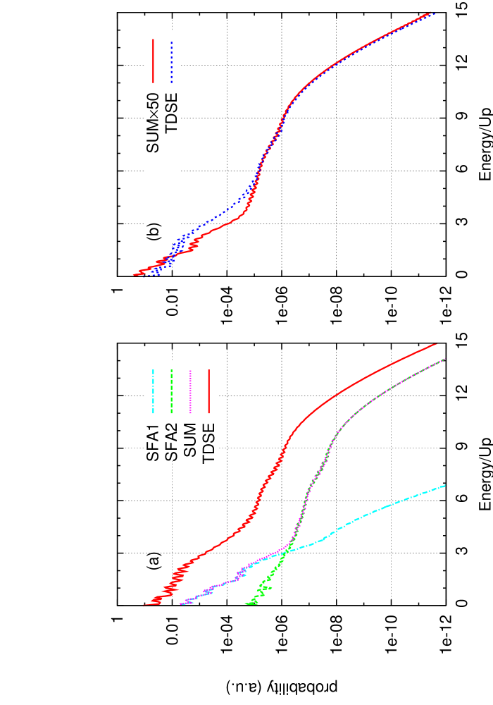
Figure 1: (Color online) Electron energy spectra for atomic hydrogen by a 5-cycle laser pulse with the wavelength of 800 nm at the peak intensity of $1.0\times 10^{14}$ W/cm².(a) From TDSE, first- (SFA1) and 2nd-order (SFA2) theory and the coherent sum of SFA1 and SFA2; (b) the sum of SFA1 and SFA2 but renormalized to the high-energy part of TDSE. Electron energy is in units of $U_{p}$, the ponderomotive energy.

We next consider the 2D electron momentum spectra. Previously theoretical calculations tend to focus on the angular distributions at specific angles, especially along the laser polarization direction Dionissopoulou97 ; bauer06 . Our goal, instead, is to examine the global 2D momentum spectra in the high-energy region and whether the spectra can be described by the SFA2. In Fig. 2 the 2D momentum spectra calculated from SFA2 and from TDSE are shown. The horizontal and the vertical axes are the electron momenta parallel and perpendicular to the laser polarization, respectively, on a plane containing the polarization axis. Since the electron yield drops very rapidly with energy (see Fig. 1), to make the high energy part visible, the 2D momentum distributions in each frame have been renormalized such that the total ionization yield at each electron energy is the same. At first glance, clearly the two frames look very similar in the high-momentum region. (The difference in the small momentum part is not important since SFA1 is dominant there.) Similar agreement has also been observed for lasers of different intensities and wavelengths.

The striking features of Fig. 2 are the two half circles on each side of the origin. The center of each circle is shifted along the $p_{\parallel}(=p_{z})$ axis. We call these circular rings back rescattered ridge (BRR), representing electrons that have been rescattered into the backward directions by the target ion. Based on the results from TDSE calculations, we have confirmed torunew that the electron yields on the BRR can be interpreted as elastic scattering of the returning electrons by the target ion potential. Since the main features of the BRR are also reproduced in the SFA2 we seek to provide theoretical grounds for this interpretation.

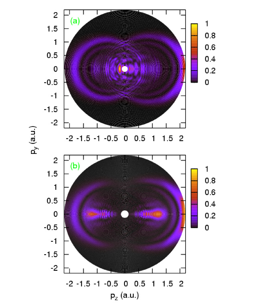
Figure 2: (Color online) Photoelectron 2D momentum distributions parallel ($p_{\parallel}=p_{z}$) and perpendicular ($p_{y}$) to the laser polarization direction for atomic hydrogen by a 5-cycle laser pulse with the wavelength of 800 nm at the peak intensity of $1.0\times 10^{14}$ W/cm². (a) SFA2 and (b) TDSE.

Evidence of these BRR electrons had been seen observed previously. Using 50-ps, 1.05-${\mu}$m linearly polarized laser pulses, Yang et al. yang93 observed unexpected narrow lobes in the angular distributions at approximately 45^∘ off the polarization axis in the high order ATI spectrum around $9U_{p}$ in single ionization of Xe and Kr atoms. The origin of the sidelobes has been analyzed by Paulus et al. Paulus_JPB94 in a two-step classical model and by Lewenstein et al. lew2 using a quasiclassical analysis. Similar theoretical analysis of these narrow sidelobes has been made by Dionissopoulou et al. Dionissopoulou97 . However, direct connection of these narrow sidelobes with the backscattering of the returning electrons has not been established at the quantitative level so far.

III.2 Analysis of the high-energy 2D momentum spectra

To identify that rescattering is responsible for the high-energy BRR electrons, in Fig. 3 we show the renormalized 2D momentum spectra for 2-cycle and 3-cycle 800 nm pulses at peak intensity of $1.0\times 10^{14}$ W/cm², with the corresponding electric fields and vector potentials plotted on the right side. The data in the 2D momentum spectra are integrated over the azimuthal angle around the polarization vector, as in (25). This presentation forces the distribution to go to zero on the $p_{\parallel}$ axis.

Consider the 2-cycle pulse, from Fig. 3(b) the electric field $E(t)$ reaches local maximum at time $t=-0.4\tau$, 0, and $0.4\tau$, where $\tau=2\pi/\omega$ is the period of the laser. Based on classical theory, electrons that are ”born” near the peak of the electric field (more precisely, at the phase angle of 17^∘ after the peak) will be driven back to the target ion about three quarters of a cycle later. Consider an electron that was born at the time $t_{b}$ near $-0.4\tau$ where the electric field strength is maximum. We will choose the convention that positive $z$ is the right side and negative $z$ the left side. The released electron is in a negative electric field so it will first moves to the right side. After the electric field changes to positive, the electron will be decelerated and may be driven back toward the target. Simple classical calculation shows that it will return to the origin at time $t_{r}$ near $0.25\tau$ where the electric field returns to zero. If this electron is scattered in the forward direction, it will be decelerated by the subsequent negative electric field for $t>t_{r}$ and ending up with low energy. On the other hand, if the electron is backscattered elastically, it will be further accelerated by the laser’s electric field and ending up with high energy. This effect on the electron momentum is obtained by adding the instantaneous vector potential ${\bf A}_{r}\equiv{\bf A}(t_{r})$ to the canonical momentum ${\bf p}$, analogous to the ”streaking” of an electron generated by an X-ray attosecond pulse in the presence of a femtosecond IR pulse auger . The shift of the center of the BRR is a measure of the magnitude of ${\bf A}_{r}$, and the radius of the circle is related to the maximum electron’s returning energy $3.17U_{p}$. In Fig. 3(b), electrons that are born near $t=0$, would return at about $t=0.75\tau$ where the vector potential and the electric field are near zero, thus no high-energy electrons would emerge. This explains why there is no BRR on the left side of Fig. 3(a) for the 2-cycle pulse.

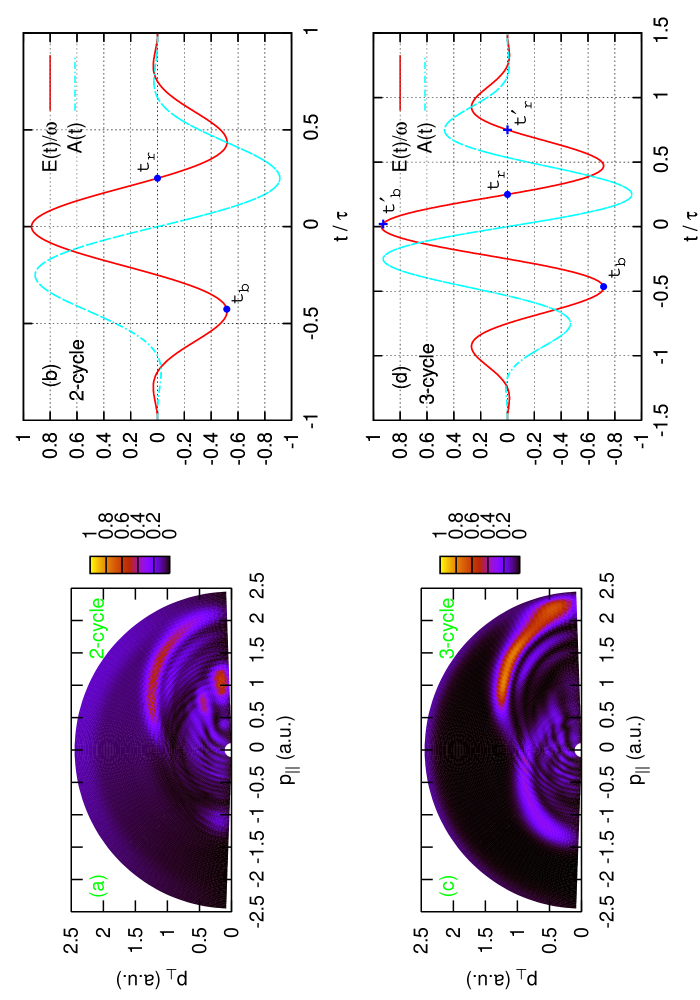
Figure 3: (Color online) Photoelectron 2D momentum distributions parallel ($p_{\parallel}=p_{z}$) and perpendicular ($p_{\perp}=\sqrt{p_{x}^{2}+p_{y}^{2}}$) to the laser polarization direction for atomic hydrogen by laser pulses at the peak intensity of $1.0\times 10^{14}$ W/cm² with the wavelength of 800 nm for durations of 2 cycles and 3 cycles, respectively. The corresponding laser fields and vector potentials are shown on the right for the analysis of the rescattering mechanism.

Consider next the 3-cycle pulse, the right BRR is due to ionization occurs near $t_{b}$ and returns near $t_{r}$ as before. The BRR on the left is due to ionization near $t^{\prime}_{b}$ and returns near $t^{\prime}_{r}$. Since the vector potential at $t^{\prime}_{r}$ is smaller than that at $t_{r}$, the shift of the center and the radius of the circle of the left BRR are smaller.

One advantage of the SFA2 is that it allows us to identify the born time and the returning time directly. To analyze the right-side BRR in Fig. 3(c), we set ”window functions” such that the born time is restricted to $[-0.5\tau,-0.4\tau]$ for $t^{\prime}$ and the return time interval $[0,0.75\tau]$ for $t$ in (20), as shown in Fig. 4(b). The resulting 2D spectra shown in Fig. 4(a) is similar to the right side of the 2D spectra in Fig. 3(c), confirming that the right BRR is from electrons born near $t_{b}$. Similarly, in Fig. 4(c), the 2D momentum distributions are presented to identify the left-side ridge by setting the born time interval $[0,0.1\tau]$ for $t^{\prime}$ and the returning time interval $[0.5\tau,1.5\tau]$ for $t$ in (20), as shown in Fig. 4(d). The resulting left BRR is also similar to the one in Fig. 3(c). These confirm our interpretation of the origin of each BRR, in terms of its born time and returning time.

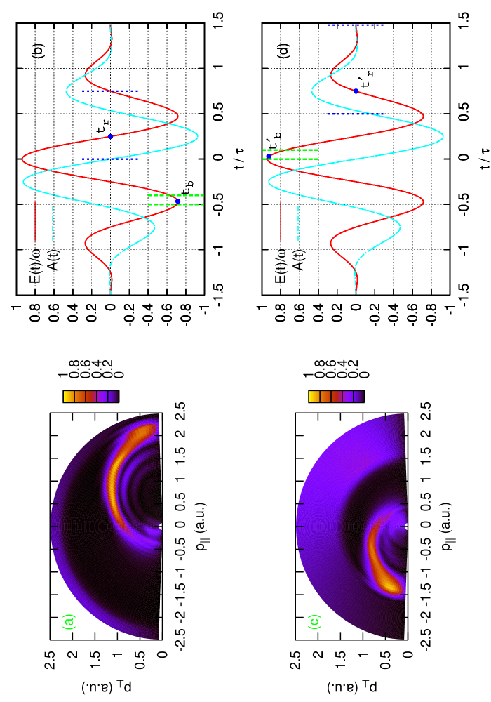
Figure 4: (Color online) Analysis of 2D momentum distributions as in Fig. 3 for the 3-cycle pulse, for the identification of the tunneling time and rescattering time, for the right- and left-side BRR electrons. See text.

The position of the BRR in the 2D momentum space can be expressed as

$${\textbf{p}}=-{\textbf{A}}_{r}+{\textbf{p}}_{r}$$ (27)

where ${\textbf{p}}_{r}$ is momentum vector measured from the center of the circle which is located at $-{\textbf{A}}_{r}$ and hence $p_{r}$ is the radius of the BRR. The projection of the photoelectron momentum in the parallel and perpendicular directions are

$$p_{||} = p\cos\theta=-A_{r}-p_{r}\cos\theta_{r}$$

$$p_{\perp} = p\sin\theta=p_{r}\sin\theta_{r}$$ (28)

where $\theta_{r}$ is the backscattering angle, ranging from 90^∘ to 180^∘.

Actually, the BRR in the 2D momentum distribution is formed by the cutoff peak in the angle-resolved energy spectra. To check the accuracy of the interpretation represented by (27), we ”measured” the center position and the radius of the right-side BRR as $|A_{r}|=0.93$, $p_{r}=1.18$ in the 2D momentum distributions shown in Fig 2. We chose $\theta_{r}=180^{\circ}$, $160^{\circ}$, $140^{\circ}$, and $120^{\circ}$, which correspond to $\theta=0^{\circ}$, $11.2^{\circ}$, $22.5^{\circ}$, and $34^{\circ}$, with the corresponding energies of 2.19, 2.13, 1.94, and 1.65, respectively. In Fig. 5, we show the angle-resolved energy spectra at these angles with the predicted electron energies by arrows. The arrows indeed are located at the peak positions of the angle-resolved energy spectra.

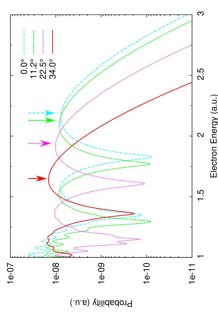
Figure 5: (Color online) Angle-resolved energy spectra for atomic hydrogen by a 5-cycle laser pulse with the wavelength of 800 nm at the peak intensity of $1.0\times 10^{14}$ W/cm², for four detector angles of $\theta=0^{\circ}$, $11.2^{\circ}$, $22.5^{\circ}$, and $34^{\circ}$, respectively. The arrows indicate the energies predicted by equation (III.2), see text for detail.

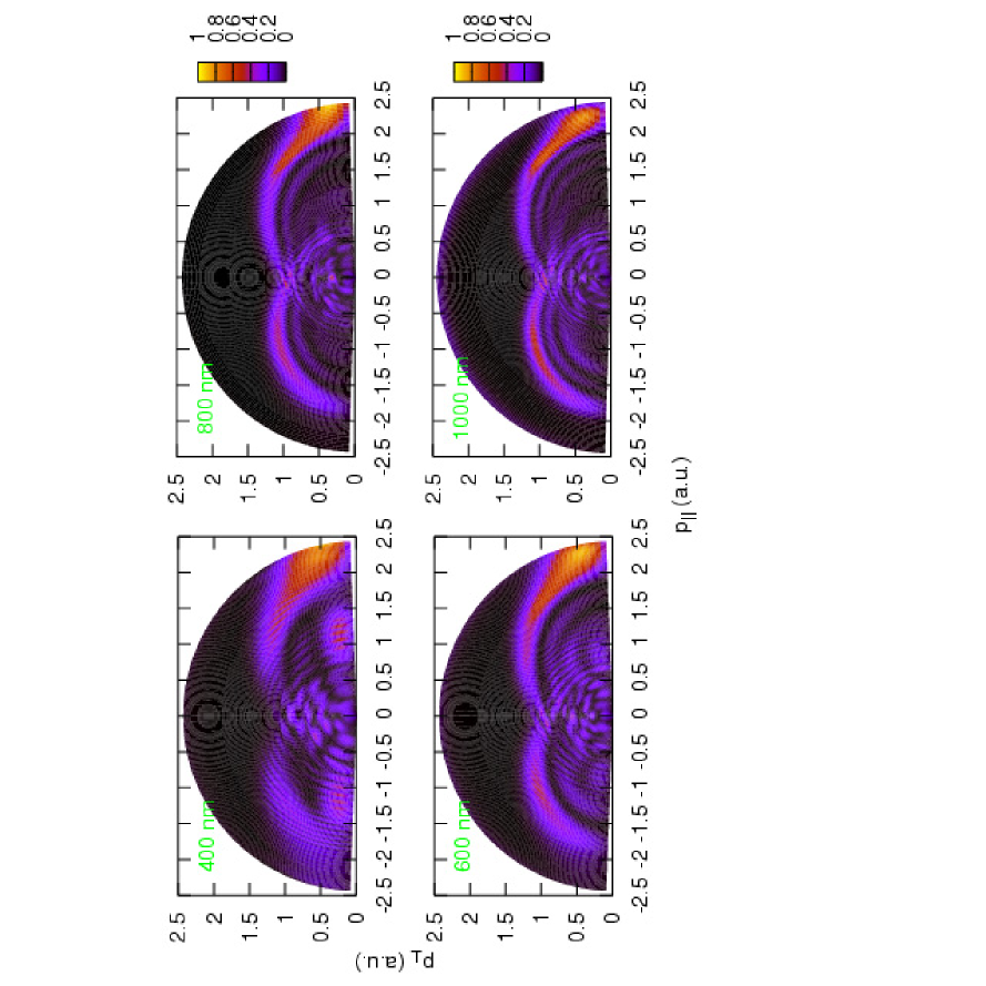
Figure 6: (Color online) 2D momentum distributions for atomic hydrogen by 5-cycle laser pulses with the same Keldysh parameter $\gamma=1.07$, but for wavelengths of 400, 600, 800, and 1000 nm, respectively.

According to the previous paragraph, the BRR depends on the vector potential of the pulse only. In Fig. 6, we show the renormalized 2D momentum spectra for single ionization of hydrogen atom by 5-cycle laser pulses with fixed Keldysh parameter $\gamma=1.07$. The wavelengths are 400, 600, 800, and 1000 nm, and the corresponding peak intensities are $4.0\times 10^{14}$, $1.78\times 10^{14}$, $1.0\times 10^{14}$, and $6.4\times 10^{13}$ W/cm², respectively. It can be seen from Fig. 6 that the BRR’s exist for all the cases and the 2D spectra appear to be very similar to each other. It can also be seen in Fig. 6 that the BRR breaks into sub-rings and the width of the BRR becomes narrower with increase of wavelength. These sub-rings are not investigated here.

III.3 Returning electron wave packets

By identifying the BRR electrons as due to the backscattering of the returning electrons by the target ion, the yield along the BRR should then be proportional to the differential elastic cross sections of electrons by the target ion. Within the SFA2, the elastic scattering is treated in the Born approximation, where the scattering amplitude is proportional to the Fourier transform of the ion potential

$$V(\textbf{q})=-\frac{1}{4\pi}\int\exp(i\mathbf{q}\cdot\textbf{r})V(\textbf{r})d\textbf{r},$$ (29)

here q is the momentum transfer which is related to the rescattering angle $\theta_{r}$ and the radius $p_{r}$ of the BRR by

$$q=2p_{r}\sin(\theta_{r}/2).$$ (30)

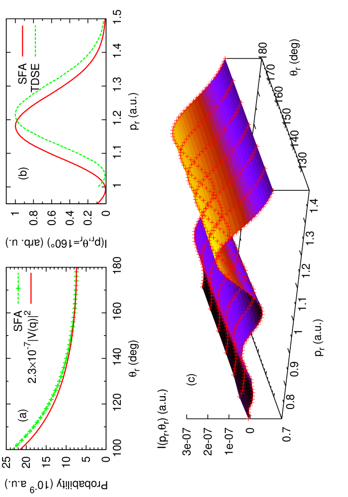
Figure 7: (Color online) Right-side BRR for atomic hydrogen by a 5-cycle laser pulse at the peak intensity of $1.0\times 10^{14}$ W/cm² with the wavelength of 800 nm. (a) Comparison of the first Born elastic scattering cross sections with the angular distributions on BRR calculated from SFA2; (b) Comparison of the electron wave packet from SFA2 with that from TDSE at $\theta_{r}=160^{\circ}$; (c) The wave packets of the returning electrons are shown to be independent of the scattering angles.

Fig. 7(a) shows the comparison of the first Born electron elastic scattering cross sections with the angular distributions on the right-side BRR in the 2D momentum spectra shown in Fig. 2(a). For the comparison presented in Fig. 7(a), the radius of BRR is taken to be $p_{r}=1.2$. It can be seen that for $\theta_{r}>100^{\circ}$, the differential elastic scattering cross sections are very close to the photoelectron angular distributions along BRR, indicating that elastic scattering of electrons by the parent ion can be extracted from the angular distribution along the BRR.

Expanding the rescattering idea further, we then ask if it is possible to treat the electron yield on the BRR as due to the backscattering of a returning electron wave packet. To test this idea, we write

$$\frac{\partial^{2}P}{\partial E\partial\hat{\textbf{p}}}|_{\varphi=\text{cons}}=I(p_{r},\theta_{r})|V(\textbf{q})|^{2}.$$ (31)

On the left side in (31), the angular distribution is obtained on any plane containing the $z$ axis in the momentum space due to the cylindrical symmetry. Note that $|V(\textbf{q})|^{2}$ is the elastic differential cross section for each ion by an electron with energy $E_{r}=p_{r}^{2}/2$ (see (30)) while the actual energy of electron in the laser field is $E=[-{\textbf{A}}_{r}+{\textbf{p}}_{r}]^{2}/2$. In Fig. 7(b), we show the extracted $I(p_{r},\theta_{r})$ at the angle of $\theta_{r}=160^{\circ}$ from the right-side BRR in Fig. 2. The wave packet extracted from SFA2 is essentially identical to that from the TDSE except for a small shift of the center from 1.18 to 1.21. Here, we see that the radius of BRR is determined by the center of the wave packet.

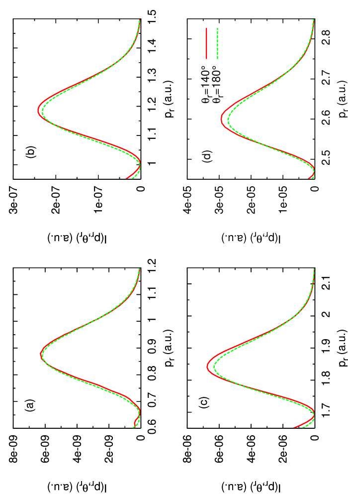
Figure 8: (Color online) Distributions of the momentum of the right-side BRR electrons for atomic hydrogen by 5-cycle laser pulses with the wavelength of 800 nm at the peak intensities of (a) $5.0\times 10^{13}$, (b) $1.0\times 10^{14}$, (c) $2.5\times 10^{14}$, and (d) $5.0\times 10^{14}$ W/cm².

According to the classical or semiclassical theory the maximal energy of the returning electron is $3.17U_{p}$. Extending this idea for each optical cycle, we then have $E_{r}=p_{r}^{2}/2=3.17\bar{U}_{p}$, where $\bar{U}_{p}=A_{r}^{2}/4$. Consequently, we get

$$p_{r}=1.26A_{r}.$$ (32)

For a 5-cycle laser pulse at the peak intensity of $1.0\times 10^{14}$ W/cm² with the wavelength of 800 nm, $A_{r}=0.93$ for the right-side BRR, corresponding to $p_{r}=1.17$, which agrees with the SFA2 calculation.

The wave packet extracted from (31) should not depend on $\theta_{r}$ if the electron on the BRR comes entirely from the backscattering when the scattering angle is large. We found this is the case for $\theta_{r}>120^{\circ}$, as plotted in Fig. 7(c).

We next check the relation (32) for different intensities. In Fig. 8 are presented the wave packets extracted from the right-side BRR for the photoelectrons generated by 5-cycle, 800nm laser pulses for peak intensities of 0.5, 1.0, 2,5 and $5.0\times 10^{14}$ W/cm². First we note that the wave packets derived from the two scattering angles are nearly the same. For these pulses, the vector potentials at the return time have values $A_{r}=0.65$, 0.93, 1.46 and 2.08, respectively. From (32), the radii are calculated to be $p_{r}=0.82$, 1.17, 1.84 and 2.62, which compare well with the peak positions of 0.86, 1.18, 1.84 and 2.60, from the extracted electron wave packets shown in Fig. 8.

III.4 Returning electron wave packet for long pulses

The analysis of BRR so far has been limited to short pulses. For longer pulses, the BRR electrons on each side can be generated from several born times, each separated from the previous one by one full optical cycle. Interference from these coherent electron bursts results in the characteristic ATI peaks.

In Fig. 9, we show the SFA2 results for 10- and 20-cycle pulses at the peak intensity of $1.0\times 10^{14}$ W/cm² and wavelength of 800 nm. For these ”long” pulses, accurate TDSE results are difficult to obtain. Figs. 9(a) and (b) show that the electron yields on the BRR are oscillatory, but the envelope is well reproduced by the differential elastic scattering cross sections. The oscillations are attributed to the electron wave packets, see Figs. 9(c) and (d). Note that the envelopes of the electron wave packets in these two figures are similar to the smooth wave packet for the 5-cycle pulse shown in Fig. 7(b). The peak positions of the envelopes for 10- and 20-cycle pulses are at 1.16 and 1.17, respectively from the figure, as compared to 1.17 from Fig. 7(b).

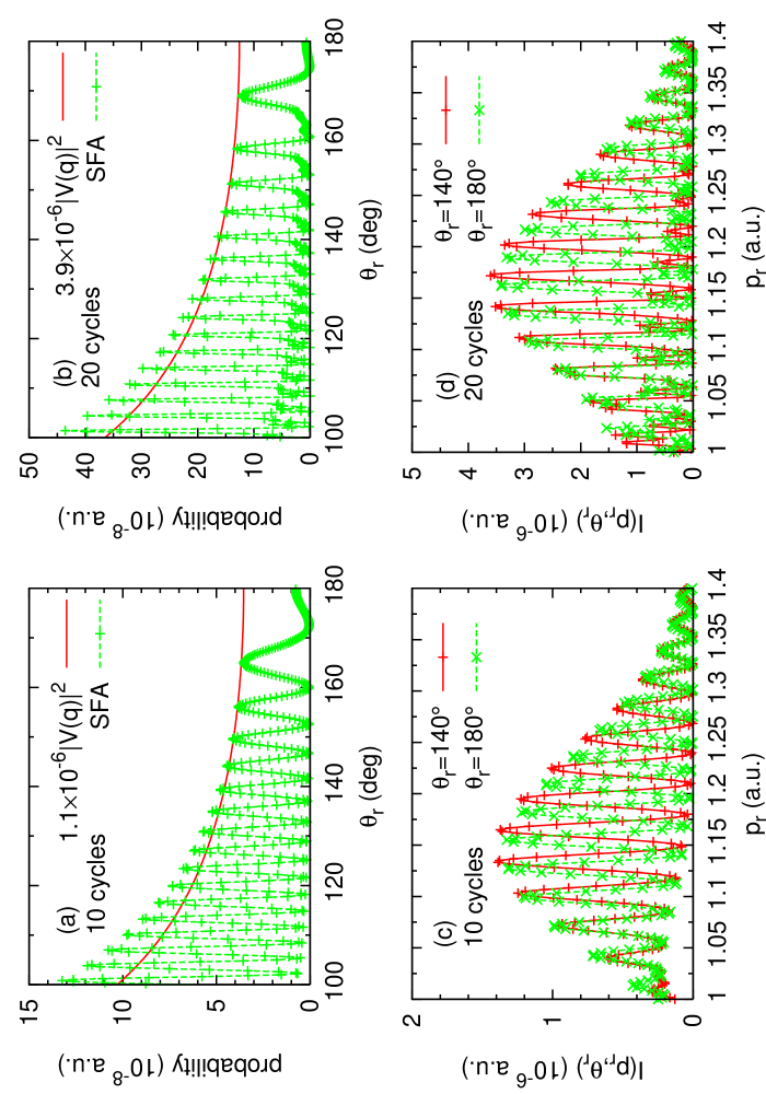
Figure 9: Ionization of hydrogen by laser pulses at the peak intensity of $1.0\times 10^{14}$ W/cm² with the wavelength of 800 nm and the full durations of 10 and 20 cycles. (a,b): Comparison of the first Born elastic scattering cross sections with the SFA2 angular distributions of the BRR electrons; (c,d): Distributions of $I(p_{r},\theta_{r})$ at $\theta_{r}=140^{\circ}$ and $180^{\circ}$.

For long pulses, electrons which have been released earlier may return at different times. So far we have considered the dominant first return. For later returns it is generally believed that the probabilities would be smaller since the electron wave packet expected to spread in time. Based on the SFA2, we can estimate the wave packets for the first and the later returns. For this purpose, we consider a 25-cycle pulse. We assume that the electrons are born in the interval $[-0.5\tau,-0.4\tau]$. For the first return we isolate backscattering occurring within the time interval $[0.0,0.5\tau]$. For the second and the third returns, the intervals are chose to be $[0.5\tau,1.0\tau]$ and $[1.0\tau,1.5\tau]$, respectively, i.e., each is half an optical cycle later from the previous return. From the calculated 2D spectra for each return, we extracted the electron wave packets, see Fig. 10. It is clear that the wave packet from the first return has the highest yield and highest momentum. The wave packet from second return has lower momentum than from the third return, but the peak intensity is about twice higher. The wave packets ”derived” from this model are qualitatively similar to those obtained from the classical simulation by Tong et al tong93pra , but with larger width and smaller strength since spreading of the wave packet is included in the SFA2 but not in the classical simulation of the latter.

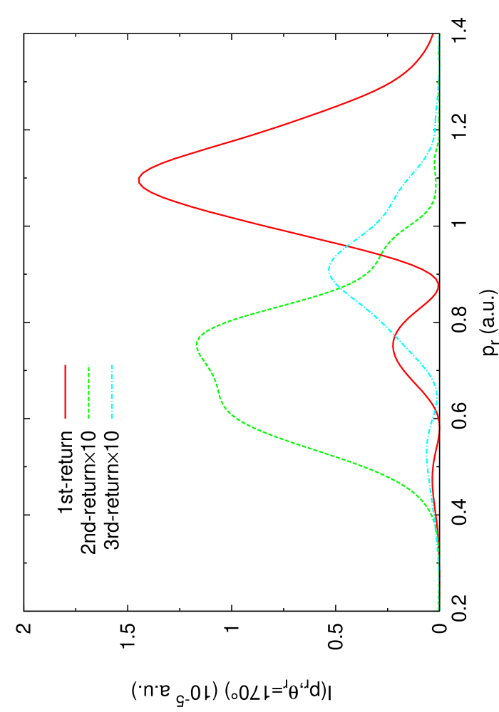
Figure 10: Distributions of $I(p_{r},\theta_{r})$ of the BRR electrons, born at the time ($-0.5\tau$, $-0.4\tau$) and returning at the 1st-return time (0.0, $0.5\tau$), the 2nd-return time ($0.5\tau$, $1.0\tau$) and the 3rd-return time ($1.0\tau$, $1.5\tau$), at $\theta_{r}=170^{\circ}$ for ionization of hydrogen by a 25-cycle laser pulse at the peak intensity of $1.0\times 10^{14}$ W/cm² with the wavelength of 800 nm.

IV Summary

In this paper we studied the two-dimensional momentum spectra of high-energy photoelectrons of a hydrogen atom in an intense laser pulse. We focussed on electrons that are on the back rescattered ridges (BRR). These electrons have been identified initially from solving the time-dependent Schrödinger equation (TDSE) and they were interpreted as due to the backscattering of the returning electrons by the target ion. Using the second order strong field approximation (SFA2) where the rescattering is accounted for to the first order, we showed that BRR electrons also appear in the SFA2 calculation. By analyzing the results from SFA2 we have been able to identify the time of birth of the electrons and the return time where these electrons are backscattered by the target ion. From the yields of the electrons along the BRR, we further showed that it is possible to extract the returning electron wave packet as well as the elastic scattering cross sections between the returning electrons and the target ion. The electron wave packets extracted from SFA2 have been shown to be very close to those extracted from solving the TDSE. Since the SFA2 calculation is much simpler, this allows us to analyze the returning electron wave packets conveniently for laser pulses of different intensities and durations. We comment that the yield along the BRR calculated using the SFA2 does not predict the correct elastic scattering cross section between the electron and the target ion since it was based on the first order theory. For the present atomic hydrogen target, on the other hand, the elastic scattering cross sections calculated from the first-order theory and the exact results are identical – a special property of the Coulomb potential. While results have been presented here only for atomic hydrogen target, similar comparison with the same conclusion has been made for other atoms. In addition, there is no reason to expect that the same conclusion would not hold for molecular targets where accurate TDSE solutions at the same level of accuracy as in atoms is computationally not feasible.

V Acknowledgment

This work was supported in part by Chemical Sciences, Geosciences and Biosciences Division, Office of Basic Energy Sciences, Office of Science, US Department of Energy. TM is also supported by financial aids from the research fund of the University of Electro-communications,the 21st century COE program on ”Coherent Optical Science” and the Ministry of Education, Culture, Sports, Science, and Technology, Japan.

References

- (1) R. R. Freeman, P. H. Bucksbaum, H. Milchberg, S. Darack, D. Schumacher, and M. E. Geusic, Phys. Rev. Lett. 59, 1092 (1987).
- (2) M. Wickenhauser, X. M. Tong and C. D. Lin, Phys. Rev. A 73, 011401(R) (2006).
- (3) J. N. Bardsley, A. Szoke, and M. J. Comella, J. Phys. B 21, 3899 (1988).
- (4) R. Wiehle, B. Witzel, H. Helm, and E. Cormier, Phys. Rev. A 67, 063405 (2003).
- (5) A. Rudenko, K. Zrost, C. D. Schröter, V. L. B. de Jesus, B. Feuerstein, R. Moshammer, and J. Ullrich, J. Phys. B 37, L407 (2004).
- (6) C. M. Maharjan, A. S. Alnaser, I Litvinyuk, P. Ranitovic, and C. L. Cocke, J. Phys. B 39, 1955 (2006).
- (7) Z. Chen, T. Morishita, A.-T. Le, M. Wickenhauser, X. M. Tong, and C. D. Lin, Phys. Rev. A 74, 053405 (2006).
- (8) D. C. Arbó, S. Yoshida, E. Persson, K. I. Dimitriou, and J. Burgdöorfer, Phys. Rev. Lett. 96, 143003 (2006).
- (9) T. Morishita, Z. Chen, S. Watanabe, and C. D. Lin, Phys. Rev. A 75, 023407 (2007).
- (10) M. P. Hertlein, P. H. Bucksbaum, and H. G. Muller, J. Phys. B 30, L197 (1997).
- (11) G. G. Paulus, F. Grasbon, H. Walther, R. Kopold, and W. Becker, Phys. Rev. A 64, 021401 (2001)
- (12) H. G. Muller and F. C. Kooiman, Phys. Rev. Lett. 81, 1207 (1998).
- (13) J. Wassaf, V. Véniard, R. Taïeb, and A. Maquet, Phys. Rev. Lett. 90,013003 (2003).
- (14) R. Kopold, W. Becker, M. Kleber and G. G. Paulus, J. Phys. B 35, 217 (2002).
- (15) B. Borca, M. V. Frolov, N. L. Manakov, and A. F. Starace, Phys. Rev. Lett. 88,193001 (2002).
- (16) T. Morishita, A.-T. Le, Z. Chen, and C. D. Lin, Science (submitted)
- (17) L. V. Keldysh, Sov. Phys. JETP 20, 1307 (1964).
- (18) M. Lewenstein, K. C. Kulander, K. J. Schafer, and P. H. Bucksbaum, Phys. Rev. A 51, 1495 (1995).
- (19) D. B. Milošević, G. G. Paulus, and W. Becker, Optics Express 11, 1418 (2003).
- (20) D. B. Milošević, A. Gazibegović-Busuladžić, and W. Becker, Phys. Rev. A 68, 050702(R) (2003).
- (21) A. Gazibegović-Busuladžić, D. B. Milošević, and W. Becker, Phys. Rev. A 70, 053403 (2004).
- (22) D. B. Milosevic, G. G. Paulus, and W. Becker, Phys. Rev. A 71, 061404(R) (2005).
- (23) A. Becker and F. H. M. Faisal, J. Phys. B 38, R1 (2005).
- (24) X. M. Tong, K. Hino, and N. Toshima1 Phys. Rev. A 74, 031405(R) (2006).
- (25) S. Dionissopoulou, Th. Mercouris, A. Lyras, and C. A. Nicolaides, Phys. Rev. A 55, 4397 (1997).
- (26) D. Bauer, D. B. Milosevic, and W. Becker, J. Mod. Opt. 53 135 (2006).
- (27) B. Yang, K. J. Schafer, B. Walker, K. C. Kulander, P. Agostini, and L. F. DiMauro, Phys. Rev. Lett. 71, 3770 (1993).
- (28) G. G. Paulus, W. Becker, W. Nicklich, and H. Walter, J. Phys. B 27, L703 (1994).
- (29) M. Drescher, M. Hentschel, R. Kienberger, M. Uiberacker, V. Yakovlev, A. Scrinzi1, Th. Westerwalbesloh, U. Kleineberg, U. Heinzmann and F. Krausz, Nature (London) 419, 803 (2002)
- (30) X. M. Tong, Z. X. Zhao and C. D. Lin, Phys. Rev. A 68, 043412 (1993).