Expansion of the Planet Detection Channels in Next-Generation Microlensing Surveys

Abstract

We classify various types of planetary lensing signals and the channels of detecting them. We estimate the relative frequencies of planet detections through the individual channels with special emphasis on the new channels to be additionally provided by future lensing experiments that will survey wide fields continuously at high cadence by using very large-format imaging cameras. From this investigation, we find that the fraction of wide-separation planets that would be discovered through the new channels of detecting planetary signals as independent and repeating events would be substantial. We estimate that the fraction of planets detectable through the new channels would comprise $\sim 15$ – 30% of all planets depending on the models of the planetary separation distribution and mass ratios of planets. Considering that a significant fraction of planets might exist in the form of free-floating planets, the frequency of planets to be detected through the new channel would be even higher. With the expansion of the channels of detecting planet, future lensing surveys will greatly expand the range of planets to be probed.

1. Introduction

Microlensing is one of the important techniques that can detect and characterize extrasolar planets. The technique is important especially in the detections of low-mass planets and it is possible to detect Earth-mass planets from ground-based observations. The capability of the microlensing technique has been demonstrated by the recent detections of four planets (Bond et al., 2004; Udalski et al., 2005; Beaulieu et al., 2006; Gould et al., 2006). Among them, one (OGLE-2005-BLG-390Lb) is the lowest mass planet ever detected among those orbiting normal stars.

Planetary lensing signal lasts a short period of time; several days for a Jupiter-mass planet and several hours for an Earth-mass planet. To achieve the observational frequency required for the detection of the short-lived planetary signal, current microlensing planet search experiments are being operated in an observational setup, where survey observations (e.g., OGLE: Udalski (2003), MOA: Bond et al. (2002)) issue alerts of ongoing events and subsequent follow-up observations (e.g., PLANET: Albrow et al. (2001), MicroFUN: Dong et al. (2006)) intensively monitor the alerted events. Under this strategy, however, only planetary signals occurring during the lensing magnification of the source star can be effectively monitored. These signals are produced by planets having projected separations from the star similar to the Einstein radius of the primary star. As a result, only planets located in a narrow region of separation from the host star can be effectively detected under the current planetary lensing searches.

The range of planets detectable with the microlensing technique will be expanded with next-generation lensing experiments that will survey wide fields continuously at high cadence by using very large-format imaging cameras. Several such surveys in space and on ground are being seriously considered. Microlensing Planet Finder (MPF), that succeeds the original concept of Galactic Exoplanet Survey Telescope (GEST) (Bennett & Rhie, 2002), is a space mission proposed to NASA’s Discovery Program with the main goal of searching for a large sample of extrasolar planets by using gravitation lensing technique (Bennett, 2004). The ‘Earth-Hunter’ project is a ground-based microlensing survey that plans to achieve $\sim 10$ minute sampling by using a distributed network of multiple wide-field ($\sim 2^{\circ}\times 2^{\circ}$) telescopes (A. Gould, private communication). Recently, the MOA group begin a strategy observing a fraction of their fields very frequently by using a recently upgraded 1.8 m telescope with a $2.2\ {\rm deg}^{2}$ field of view. These surveys dispense with the alert/follow-up mode of searching for planets and instead simultaneously obtain densely and continuously sampled light curves of all microlensing events in the field-of-view. With these surveys, the efficiency of planet detection will greatly improve thanks to the enhanced monitoring frequency and continuous sampling. In addition, the future lensing experiments will be able to open new channels of planet detections because source stars are monitored regardless of their magnifications. In this paper, we classify various channels of detecting planetary lensing signals and estimate the relative frequencies of planet detections through the individual channels with special emphasis on the new channels that will be provided by future lensing surveys.

The format of the paper is as follows. In § 2, we describe basics of planetary microlensing. In § 3, we present various types of planetary lensing perturbations and classify the channels of detecting them. In § 4, we estimate the relative frequencies of detecting planets through the individual channels. We discuss the importance of the new planet detection channels to be provided by future lensing surveys. We summarize the results and conclude in § 5.

2. Basics of Planetary Microlensing

Due to the existence of a planetary companion, description of the planetary lensing behavior requires formalism of binary lensing (Witt, 1990; Witt & Mao, 1995). Because of the small mass ratio of the planet, the light curve of a planetary lensing event is well described by that of a single lens of the primary star for most of the event duration. However, a short-duration perturbation can occur when the source star passes the region around the caustics. The caustics are important features of binary lensing and they represent the set of source positions at which the magnification of a point source becomes infinite. The caustics of binary lensing form a single or multiple sets of closed curves where each of which is composed of concave curves (fold caustics) that meet at points (cusps). For a planetary case, there exist two sets of disconnected caustics: ‘central’ and ‘planetary’ caustics.

The single central caustic is located close to the host star. It has a wedge shape with four cusps, where two are located on the star-planet axis and the other two are located off the axis. The size of the central caustic as measured by the separation between the on-axis cusps is represented by (Chung et al., 2006)

$$\Delta\xi_{\rm cc}\sim{4q\over(s-s^{-1})^{2}},$$ (1)

where $q$ is the planet/star mass ratio and $s$ is the star-planet separation normalized by the Einstein radius of the planetary lens system, $\theta_{\rm E}$. Then the caustic size becomes maximum when $s\sim 1.0$. In the limiting case of a very wide-separation planet ($s\gg 1.0$) and a close-in planet ($s\ll 1.0$), the caustic size decreases, respectively, as

$$\Delta\xi_{\rm cc}\propto\cases{s^{-2}&for $s\gg 1.0$,\cr s^{2}&for $s\ll 1.0$.\cr}$$ (2)

For a given mass ratio, a pair of central caustics with separations $s$ and $s^{-1}$ are identical to the first order of the approximation where the planet-induced anomalies is treated as a perturbation (Dominik, 1999; Griest & Safizadeh, 1998; An, 2005). The central caustic is always smaller than the planetary caustic. Since the central caustic is located close to the primary lens, the perturbation induced by the central caustic always occurs near the peak of high-magnification events.

The planetary caustic is located away from the host star. The center of the planetary caustic is located on the star-planet axis and the position vector to the center of the planetary caustic from the primary lens position is related to the lens-source separation vector, ${\bf s}$, by

$${\bf r}_{\rm pc}={\bf s}\left(1-{1\over s^{2}}\right).$$ (3)

Then, the planetary caustic is located on the planet side, i.e. ${\rm sign}({\bf r}_{\rm pc})={\rm sign}({\bf s})$, when $s>1.0$, and on the opposite side, i.e. ${\rm sign}({\bf r}_{\rm pc})=-{\rm sign}({\bf s})$, when $s<1.0$. When $s>1.0$, there exists a single planetary caustic and it has a diamond shape with four cusps. When $s<1$, there are two caustics and each has a triangular shape with three cusps. The size of the planetary caustic is related to the planet parameters by

$$\Delta\xi_{\rm pc}\propto\cases{q^{1/2}\left[s(s^{2}-1)^{1/2}\right]^{-1}&for $s>1$,\cr q^{1/2}(\kappa_{0}-\kappa_{0}^{-1}+\kappa_{0}s^{-2})\cos\theta_{0}&for $s<1$,\cr}$$ (4)

where $\kappa(\theta)=\left\{[\cos 2\theta\pm(s^{4}-\sin^{2}2\theta)^{1/2}]/(s^{2}-s^{-2})\right\}^{1/2}$, $\theta_{0}=[\pi\pm\sin^{-1}(3^{1/2}s^{2}/2)]/2$, and $\kappa_{0}=\kappa(\theta_{0})$ (Han, 2006). We note that the dependence of the planetary caustic size on the mass ratio is $\Delta\xi_{\rm pc}\propto q^{1/2}$, while the dependence of the central caustic size is $\Delta\xi_{\rm cc}\propto q$. Therefore, the decay rate of the planetary caustic with the decrease of the planet mass is slower than that of the central caustic. The planetary caustic is located within the Einstein ring of the primary star when the planet is located in the range of separation from the star of $0.6\lesssim s\lesssim 1.6$. The size of the caustic is maximized when the planet is located in this range, and thus this range is called as the ‘lensing zone’ (Gould & Loeb, 1992; Griest & Safizadeh, 1998). In the limiting cases of planetary separation, the size of the planetary caustic deceases similar to the central caustic, i.e.

$$\Delta\xi_{\rm pc}\propto\cases{s^{-2}&for $s\gg 1.0$,\cr s^{2}&for $s\ll 1.0$.\cr}$$ (5)

In the limiting case of $s\ll 1.0$, the two lens components work as if they are a single lens. In the limiting case of $s\gg 1.0$, on the other hand, the star and planet work as if they are two independent lenses.

Figure 1.— Schematic representation of the planetary signals with various types. For the details of the classification scheme, see § 3.

3. Classification of Planet Detection Channels

Planetary lensing signal takes various forms depending on the characteristics of the planetary system, especially on the star-planet separation, and the source trajectory with respect to the positions of the star and planet. In this section, we classify various types of planetary lensing signals and the channels of detecting them.

Type I perturbation shows up as a perturbation to the smooth light curve of the primary-induced lensing event (see the top panel in Figure 1). This type of perturbation is produced by planets with projected star-planet separations similar to the Einstein radius of the primary star, i.e. $s\sim 1.0$. As a result, the channel of detecting planets through the detection of type I perturbation is often referred as the ‘resonant channel’. The resonant channel is the prime channel of detecting planets in current planetary lensing searches, which are based on survey/follow-up mode. Depending on whether the perturbation is induced by the planetary or central caustic, the perturbation takes place on the side or near the peak of the light curve.

Type II perturbation is produced by a planet with a projected separation from the primary star substantially larger than the Einstein radius of the primary star ($s\gg 1.0$) and it occurs when the source trajectory passes both the effective magnification regions of the primary star and planet. The planetary signal is the planet-induced lensing light curve itself that is well separated from the light curve of the primary (see the second panel in Figure 1). Since two successive events are produced by the star and planet, respectively, this channel is often referred as the ‘repeating channel’ (Di Stefano & Scalzo, 1999). The planetary signal occurs long after or before the event induced by the primary star, and thus type II perturbation is difficult to be detected by the current planetary lensing searches monitoring only during the time of primary-induced lensing magnification.

Type III perturbation is produced also by a wide-separation planet, but it occurs when the source trajectory passes only the effective magnification region of the planet. Then, the planetary signal is the independent lensing light curve produced by the planet itself (see the third panel in Figure 1). We refer this channel of planet detection as the ‘independent channel’. Type III perturbation is also difficult to be detected by the current planetary lensing searches.

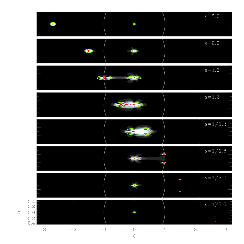
Figure 2.— Maps of planetary signal detectability as a function of the source position for planetary systems with various projected star-planet separation. The detectability is quantified as the ratio of the fractional deviation of the planetary lensing light curve from that of the single lensing event of the primary star to the photometric precision. The maps are centered at the position of the primary lens star and the planet is located on the left. The green (green curve) is drawn at the level of $D=3$. The solid circle centered at the primary star in each map represents the Einstein ring. The closed figures drawn by red curves are the caustics. All lengths are in units of the Einstein radius of the planetary system and $\xi$ and $\eta$ represent the coordinates that are parallel and normal to the star-planet axis, respectively. Each planetary perturbation region is approximated by an elliptical region and the green ellipse represents its boundary. The planetary lens system has a common planet/star mass ratio of $q=3\times 10^{-3}$.

Wide-separation planets can also be detected through another channel. Type IV perturbation is produced by a wide-separation planet and it occurs when the source trajectory passes very close to the primary star. The planetary signal is then a brief perturbation near the peak of the high-magnification lensing light curve produced by the primary star (see the fourth panel in Figure 1). We refer this channel as the ‘wide central channel’. High-magnification events are of highest-priority in the current microlensing follow-up observations because of their high sensitivity to planets (Griest & Safizadeh, 1998; Albrow et al., 2000; Bond et al., 2002; Rattenbury et al., 2002; Abe et al., 2004; Yoo et al., 2004; Dong et al., 2006) and thus type IV perturbation can be detected from current follow-up observations.

Type IV perturbation is produced by a planet with a star-planet separation substantially smaller than the Einstein radius of the primary star and it occurs when the source trajectory passes very close to the primary star. The planetary signal is very similar to the type IV perturbation (see the fourth panel in Figure 1) due to the $s\leftrightarrow s^{-1}$ symmetry of the central caustic (Dominik, 1999; An, 2005). As a result, distinguishing the two types of perturbation is often difficult, especially for perturbations induced by low-mass planets with mass ratios $q\lesssim 10^{-4}$ (Chung et al., 2006).

4. Frequency of the Individual Channels

In the previous section, we presented various types of planetary perturbations and the channels of detecting them. Then, what would be the relative frequencies of detecting planets through the individual channels from future lensing surveys? In this section, we answer to this question.

The rate of planet detection is proportional to the cross-section of the planetary perturbation region, $\sigma$. We, therefore, estimate the relative frequencies by computing the cross-sections of the planetary perturbation regions of the corresponding types. We proceed our computation according to the following procedure.

1. First, we make maps of perturbation induced by planets with various separations and mass ratios.

2. Second, we classify the types of perturbation based on the planetary separation and the location of the perturbation regions. We then estimate the average cross-sections of the perturbation regions belonging to the individual categories based on the constructed perturbation maps.

3. Finally, we compute the relative frequencies of detecting planets through the individual channels by convolving the cross-sections with the model distributions of planetary separation.

The details of the individual processes are described in the following subsections.

4.1. Maps of Planetary Signal Detectability

The map of planetary perturbation represents the region of planet-induced lensing perturbations as a function of source position. The quantity that has been often used to represent the perturbation region is the ‘fractional deviation’ of the planetary lensing light curve from that of the single lensing event of the primary star, i.e.,

$$\epsilon={A-A_{0}\over A_{0}},$$ (6)

where $A$ and $A_{0}$ represent the lensing magnifications with and without the planet, respectively. With this quantity, however, one cannot consider the variation of the photometric precision depending on the lensing magnification and source brightness. To consider this, we construct the map of perturbation with the quantity defined as the ratio of the fractional deviation, $\epsilon$, to the photometric precision, $\sigma_{\nu}$, i.e,

$${\cal D}={\left|\epsilon\right|\over\sigma_{\nu}};\qquad\sigma_{\nu}={(AF_{\nu,{\rm S}}+F_{\nu,{\rm B}})^{1/2}\over(A-1)F_{\nu,{\rm S}}},$$ (7)

where $F_{\nu,{\rm S}}$ and $F_{\nu,{\rm B}}$ represent the photon counts from the source star and blended background stars, respectively. Under this definition of the planetary perturbation, ${\cal D}=1$ implies that the planetary signal is equivalent to the photometric precision. Hereafter, we refer the quantity ${\cal D}$ as the ‘detectability’.

To construct the map of detectability, we choose a representative Galactic bulge event. Following the result of simulations of Galactic bulge events, e.g. Han & Gould (2003, 2005), we choose a representative event as the one produced by a lens with the primary lens mass of $m=0.3\ M_{\odot}$ and the distances to the lens and source of $D_{\rm L}=6$ kpc and $D_{\rm S}=8$ kpc, respectively. For the observational condition, we take the space-based lensing survey by using the MPF mission as a reference experiment. The prime target source stars to be monitored by the MPF survey are main-sequence stars and thus we choose a main-sequence source star with an $I$-band absolute magnitude of $M_{I}=4.8$, which corresponds to a K0 star. With the assumed amount of extinction toward the Galactic bulge field of $A_{I}=1.0$, this correspond to the apparent magnitude of $I=20.3$. Following the specification of the MPF mission, we assume that the photon acquisition rate is 13 photons per second for an $I=22$ star and photometry is done on each combined image with an exposure time $t_{\rm exp}=10$ minutes. We assume that blending is not important due to high resolution from space-based observation. Finite size of the source star might affect the planet detectability (Bennett & Rhie, 1996). However, the populations of planets of our interest are the ones to be detected through the new channels (i.e., repeating and independent channels) and most of them would be giant planets because of their larger cross-sections. Considering that the angular size of the source star is a few percent of the angular Einstein radius of a giant planet, finite size of the source star has little effect on the planet detectability. We therefore do not consider finite-source effect in our analysis.

Figure 2 shows constructed maps of detectability for some example planetary systems. The maps are centered at the position of the primary lens star and the planet is located on the left. The contour (green curve) is drawn at the level of $D=3$, within which the planetary signal is detected with a $3\sigma$ confidence level. The solid circle centered at the primary star in each map represents the Einstein ring and the close figure drawn by red curves represent the caustics. All lengths are normalized in units of the Einstein radius corresponding to the mass of the primary star, $\theta_{\rm E}$.

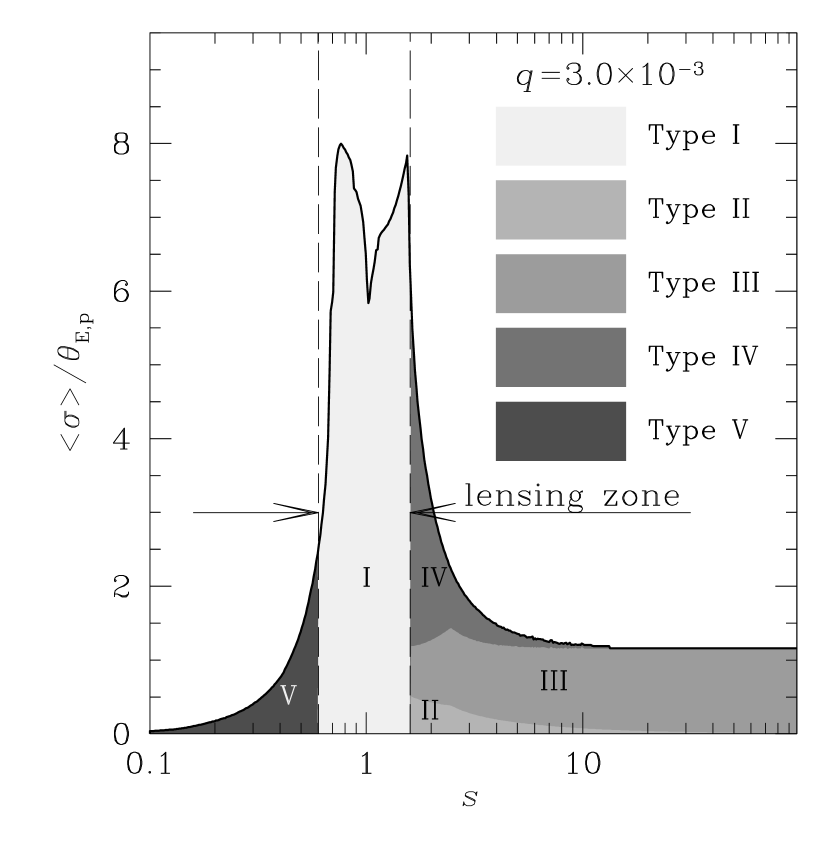
Figure 3.— Cross-section of planetary perturbation region as a function of the normalized star-planet separation. The segments marked by different tones of shade under the curve represent the types of the related planetary perturbations. We note that the cross-section is normalized by the angular Einstein radius of the planet. The assumed planet/star mass ratio is $q=3\times 10^{-3}$.

4.2. Cross-Section of Perturbation

With the constructed maps of perturbation, we then estimate the average cross-sections of the perturbation regions of the individual types. For this, we classify the types of perturbation based on the planetary separation and the location of the perturbation region.

The followings are the criteria for the classification. First, we classify all perturbations induced by planets located in the lensing zone ($0.6\leq s\leq 1.6$) into type I. If a perturbation is induced by a wide-separation ($s>1.6$) planet, the perturbation region is divided into two parts; one around the planetary caustic and the other around the central caustic. If the perturbation is caused by the central caustic, it is classified into type IV perturbation. Among the perturbations caused by the planetary caustics of wide-separation planets, the fraction of the type II perturbation is geometrically estimated as $\sin(2/\pi)\sin^{-1}(u_{\rm th}/s)$, where $u_{\rm th}$ is the radius of the effective lensing magnification region of the primary star. We adopt $u_{\rm th}=1.5$. Then the rest of perturbations induced by the planetary caustics of wide-separation planets are classified into type III. Finally, perturbations induced by planets with separations $s<0.6$ are classified into type V.

Once the types of the individual perturbation regions are determined, we then estimate the average cross-sections of the perturbation regions. A straightforward approach to estimating the cross-section would be first drawing many light curves resulting from source trajectories with various combinations of the distance to the trajectory from the center of the perturbation region and orientation angles, then checking the detectability of the planet-induced perturbations for the individual light curves, and finally estimating the cross-section as an angle-averaged value. However, this requires a large amount of computation time. Fortunately, the perturbation region is confined around caustics and its boundary is approximated by an ellipse. We therefore estimate the cross-section by approximating the perturbation region as an elliptical region. With this approximation, the cross-section of the perturbation region is estimated as the angle-averaged cross-section of the ellipse, i.e.

$$\langle\sigma\rangle={1\over\pi}\int_{0}^{\pi}\left(a_{\rm p}^{2}\sin^{2}\theta+b_{\rm p}^{2}\cos^{2}\theta\right)^{1/2}d\theta={2\over\pi}a_{\rm p}E(e),$$ (8)

where $a_{\rm p}$ and $b_{\rm p}$ are the semimajor and semiminor axes of the elliptical boundary of the perturbation region, $e=(1-b_{\rm p}^{2}/a_{\rm p}^{2})^{1/2}$ is the eccentricity of the ellipse, and $E$ represents the complete elliptical integral of the second kind. We determine the semimajor and semiminor axes of the ellipse as the widths of the perturbation region enclosed by the detectability contour with a level of $D=3$ along and normal to the star-planet axis, respectively. If the perturbation region is composed of multiple segments, we approximate the individual segments with different ellipses. In Figure 2, we present the elliptical boundaries of perturbation regions (green curves) on the top of the detectability map.

Figure 3 shows the determined cross-section of the planetary perturbation region as a function of the normalized star-planet separation for a planetary lens with a mass ratio $q=3\times 10^{-3}$, which corresponds to a Jupiter-mass planet around a primary star with a mass $m=0.3\ M_{\odot}$. We note that the cross-section is normalized by the angular Einstein radius corresponding to the mass of the planet, $\theta_{\rm E,p}=q^{1/2}\theta_{\rm E}$. The segments marked by different tones of shade under the curve represent the types of the related perturbations. From the figure, one finds that the cross-section vanishes in the limiting case of $s\rightarrow 0$. This is because the star and planet work as if they are a single lens in this limit. In the limiting case of the other end ($s\rightarrow\infty$), on the other hand, the planet acts as an independent lens and thus the cross-section converges into the value corresponding to the cross-section of the effective magnification region of the planet.

Table 1Relative Frequency

planetary separation	planet/star	types of planetary perturbation
distribution model	mass ratio	type I	type II	type III	type IV	type V
$\alpha=1.0$	$q=5.0\times 10^{-3}$	48.3%	3.8%	26.5%	12.8%	8.6%
	$q=1.0\times 10^{-3}$	56.8%	4.1%	25.9%	6.9%	6.2%
	$q=5.0\times 10^{-4}$	59.4%	4.2%	25.6%	5.4%	5.3%
	$q=1.0\times 10^{-4}$	64.3%	4.0%	24.3%	3.7%	3.7%
$\alpha=1.5$	$q=5.0\times 10^{-3}$	58.2%	2.5%	12.7%	10.0%	16.6%
	$q=1.0\times 10^{-3}$	67.2%	2.9%	12.7%	5.3%	11.9%
	$q=5.0\times 10^{-4}$	69.9%	3.0%	12.7%	4.2%	10.0%
	$q=1.0\times 10^{-4}$	75.0%	2.8%	12.1%	2.9%	7.2%

Note. — Relative frequencies of detecting planets through various channels. The frequencies are estimated under the assumption that the star-planet separation follows a power-law distribution of $dN/da\propto a^{-\alpha}$, where $\alpha$ represents the power of the distribution.

4.3. Relative Frequencies

Once the average cross-sections of the individual types of perturbation is computed, we then estimate the relative frequencies of detecting planets through the individual channels of planet detections. This is done by convolving the cross-section with model distributions of planetary separation.

We model the distribution of star-planet separation as a power-law function of the form

$${dN\over da}\propto a^{-\alpha},$$ (9)

where $a$ is the semimajor axis of the planet orbit. There is little consensus about the power of the distribution. From the analysis of observed extrasolar planets detected by radial velocity surveys, Tabachnik & Tremaine (2002) claimed $\alpha\sim 1$. On the other hand, Hayashi (1995) claimed that the surface density distribution of the minimum mass solar nebula is well described with $\alpha\sim 1.5$. We, therefore, test two different powers of $\alpha=1.0$ and 1.5. We note that larger absolute value of the power implies that planets are populated in the inner region. Then the fraction of planetary events detectable through the type I perturbation increases while the fractions through the type II, III, and IV decrease. We assume that planets are distributed up to a distance of 100 AU. Once the semimajor axis of the planet orbit is determined, the projected star-planet separation is determined under the assumption of a circular orbit and random orientation of the orbital plane. The projected separation is related to the intrinsic separation by

$$\tilde{a}=a(\sin^{2}i\cos^{2}\varphi+\cos^{2}i)^{1/2},$$ (10)

where $i$ is the inclination angle of the orbital plane and $\varphi$ is the phase of the planet on the orbital plane.

In Table 1, we present the relative frequencies of detecting planets through the individual channels. From the table, we find that the frequency of detecting planets through the new channels to be provided by future lensing surveys would be substantial. We estimate that the fraction of planets detectable through the independent and repeating channels would comprise $\sim 15$ – 30% of all planets depending on the models of the planetary separation distribution and mass ratios of planets. Considering that the total number of planets expected to be detected from five-year lensing surveys in space would be several thousands (Bennett, 2004), the number of planets detectable through the new channels would be of the order of hundred and can reach up to a thousand. We note that the estimation in Table 1 is based only on planets bound to primary stars.

The new channels to be provided by future lensing surveys are important for better understanding of planet formation and evolution processes. Planets located $\gtrsim 5$ AU from host stars could not have been detected by any of the methods currently being used for planet searches. Being able to detect planets in this range, therefore, microlensing method would provide complete sample of planets. Another population of planets that can be detected through the new channels are free-floating planets (Bennett & Rhie, 2002; Han, 2004). It is believed that a good fraction of planets have been ejected from their planetary systems during or after the epoch of planet formation (Zinnecker, 2001). Another possible origin of these planets would be the accretion of gas similar to star formation process (Boss, 2001). Since these planets were not included in our analysis, the relative frequency of planet detection through the new channels would be even larger if these planets are common.

5. Conclusion

We classified various types of planetary lensing signals and the channels of detecting them. We estimated the relative frequencies of planet detections through the individual channels with special emphasis on the new channels that will be additionally provided by future lensing surveys. From this investigation, we found that the fraction of wide-separation planets that would be discovered through the new channels of detecting planetary signals as independent and repeating events would be substantial. We estimated that the fraction of planets detectable through the new channels would comprise $\sim 15$ – 30% of all planets depending on the models of the planetary separation distribution and mass ratios of planets. Considering that a significant fraction of planets might exist in the form of free-floating planets, the frequency of planets to be detected through the new channel would be even higher. We, therefore, demonstrate that future lensing surveys will greatly expand the range of planets to be probed.

References

- Abe et al. (2004) Abe, F., et al. 2004, Science, 305, 1264
- Albrow et al. (2000) Albrow, M. D., et al. 2000, ApJ, 535, 176
- Albrow et al. (2001) Albrow, M. D., et al. 2001, ApJ, 556, L113
- An (2005) An, J. H. 2005, MNRAS, 356, 1409
- Beaulieu et al. (2006) Beaulieu, J. P., et al. 2006, Nature, 439, 437
- Bennett (2004) Bennett, D. P. 2004, BAAS, 205, 11.26
- Bennett & Rhie (1996) Bennett, D. P., & Rhie, S. H. 1996, ApJ, 472, 660
- Bennett & Rhie (2002) Bennett, D. P., & Rhie, S. H. 2002, ApJ, 574, 985
- Bond et al. (2002) Bond, I. A., et al. 2002, MNRAS, 331, L19
- Bond et al. (2002) Bond, I. A., et al. 2002, MNRAS, 333, 71
- Bond et al. (2004) Bond, I.A., et al. 2004, ApJ, 606, L155
- Boss (2001) Boss, A. P. 2001, ApJ, 551, L167
- Chung et al. (2006) Chung, S.-J., et al. 2006, ApJ, 650, 432
- Di Stefano & Scalzo (1999) Di Stefano, R., & Scalzo, R. A. 1999, ApJ, 512, 579
- Dominik (1999) Dominik, M. 1999, A&A, 349, 108
- Dong et al. (2006) Dong, S., et al. 2006, ApJ, 642, 842
- Gould & Loeb (1992) Gould, A., & Loeb, A. 1992, ApJ, 396, 104
- Gould et al. (2006) Gould, A., et al. 2006, ApJ, 644, L37
- Griest & Safizadeh (1998) Griest, K., & Safizadeh, N. 1998, ApJ, 500, 37
- Han (2004) Han, C. 2004, ApJ, 604, 372
- Han (2006) Han, C. 2006, ApJ, 638, 1080
- Han & Gould (2003) Han, C., & Gould, A. 2003, ApJ, 592, 172
- Han & Gould (2005) Han, C., & Gould, A. 2005, ApJ, 447, 53
- Hayashi (1995) Hayashi, S. S. 1995, Ap&SS, 224, 479
- Rattenbury et al. (2002) Rattenbury, N. J., Bond, I. A., Skuljan, J., & Yock, P. C. M. 2002, MNRAS, 335, 159
- Tabachnik & Tremaine (2002) Tabachnik, S., & Tremaine, S. 2002, MNRAS, 335, 151
- Udalski (2003) Udalski, A. 2003, Acta Astronomica, 53, 291
- Udalski et al. (2005) Udalski, A., et al. 2005, ApJ, 628, L109
- Witt (1990) Witt, H. J. 1990, A&A, 236, 311
- Witt & Mao (1995) Witt, H. J., & Mao, S. 1995, ApJ, 447, L105
- Yoo et al. (2004) Yoo, J., et al. 2004, ApJ, 616, 1204
- Zinnecker (2001) Zinnecker, H. 2001, Microlensing 2000: A New Era of Microlensing Astrophysics, ASP Conference Proceedings, eds. J. W. Menzies & P. D. Sackett, San Francisco, 239, 223