The Projected Rotational Velocity Distribution of a Sample of OB stars from a Calibration based on Synthetic He i lines

Abstract

We derive projected rotational velocities ($v\sin i$) for a sample of 156 Galactic OB star members of 35 clusters, H ii regions, and associations. The He i lines at $\lambda\lambda$4026, 4388, and 4471Å were analyzed in order to define a calibration of the synthetic He i full-widths at half maximum versus stellar $v\sin i$. A grid of synthetic spectra of He i line profiles was calculated in non-LTE using an extensive helium model atom and updated atomic data. The $v\sin i$’s for all stars were derived using the He i FWHM calibrations but also, for those target stars with relatively sharp lines, $v\sin i$ values were obtained from best fit synthetic spectra of up to 40 lines of C ii, N ii, O ii, Al iii, Mg ii, Si iii, and S iii. This calibration is a useful and efficient tool for estimating the projected rotational velocities of O9-B5 main-sequence stars. The distribution of $v\sin i$ for an unbiased sample of early B stars in the unbound association Cep OB2 is consistent with the distribution reported elsewhere for other unbound associations.

1 Introduction

The distribution of projected rotational velocities ($v\sin i$) of stars as a function of spectral type shows that the B-type stars have the largest average $v\sin i$ values among all main sequence stars. This observational result makes rotation especially important for early-type stars because it may affect the star’s evolution and important stellar characteristics, such as the surface abundances. Moreover, there is growing evidence that the $v\sin i$ distribution of OB stars is somehow related to the physical characteristics of the region in which they formed. These two important issues were addressed recently by, for example, Huang & Gies (2006a, b) and Wolff et al. (2007).

An approach that is frequently employed in order to obtain estimates of the projected rotational velocity consists of measuring the full-widths at half maximum (FWHM) of He i lines and adopting relationships between FWHM and $v\sin i$ established from observational data such as given by Slettebak et al. (1975); Slettebak (1982) and Howarth et al. (1997). Alternatively, the projected rotational speed can be obtained from the comparison between observational and synthetic profiles of He and metallic lines.

The goals of this contribution are to derive $v\sin i$’s for a large sample of main sequence OB stars - most of them given for the first time in the literature - and to present a calibration for $v\sin i$ versus the synthetic full-widths at half maximum of He i lines at $\lambda\lambda$4026, 4388, and 4471 Å. In Section 2 we briefly describe our observational runs and data reduction procedures. Section 3 gives the $v\sin i$ determination from the spectral synthesis of metal lines, a method that we only employed for stars with sharp lines. Section 4 details and discusses our new FWHM versus $v\sin i$ calibration, while in Section 5 we present our $v\sin i$ determinations. Finally, in Section 6 we discuss our results, paying special attention to the case of Cep OB2 association and outline some conclusions.

2 Observations

The observational data for this study are high resolution spectra of late O and early B type stars that were obtained during several observing runs between the years 1994 and 2000. The sample comprises 156 targets belonging to 35 open clusters, H ii regions, and OB associations. Table 1 lists the observed stars and their cluster membership (Columns 1 and 2). The sample of OB stars studied here for rotation was observed with the main goal of analysing radial metallicity gradients of young stars in the Galactic disk (Daflon & Cunha, 2004).

The northern stars were observed with the McDonald Observatory telescopes (University of Texas, Austin). We obtained echelle spectra (R=60,000 and spectral coverage from $\sim$4200 to $\sim$4600Å) with the 2.1-m telescope and the Sandiford Cassegrain echelle spectrometer. Lower resolution spectra (R=12,000 centered at 4340 Å) were obtained with the 2.7-m telescope and a coudé spectrometer. Details of the observations and data reduction can be found in papers by Daflon, Cunha & Becker (1999) and by Daflon et al. (2001a,b; 2003).

High resolution spectra for the southern stars in our sample were obtained with the European Southern Observatory 1.52-m telescope at La Silla, Chile, coupled with FEROS (Fiber fed Extended Range Optical Spectrograph), covering 3900-9200Å and with a resolving power $\lambda/\Delta\lambda$=48,000. (See Daflon, Cunha & Butler 2004a,b for more details). In Figure 1 we show sample FEROS spectra for the target star Sh2-47 3 in three spectral regions corresponding to the He i lines at $\lambda\lambda$4026, 4388, and 4471Å.

3 $V\sin i$ Determination via Spectrum Synthesis of Metal Lines

Stars with sharp spectral lines are best suited for abundance analyses via either equivalent width measurements or spectrum synthesis. When line spectrum synthesis is adopted to derive the elemental abundances, the corresponding value of the stellar projected velocity is also obtained. A significant fraction of the targets studied here (69 stars) had low enough values of rotational projected velocities so that their abundances could be derived via spectrum synthesis of a number of spectral lines. The synthetic spectra were computed in non-LTE using the codes detail (Giddings, 1981) and surface (Butler & Giddings, 1985) plus line-blanketed LTE atlas9 model atmospheres (Kurucz,, 1993). The model atoms adopted in the calculations were taken from Eber & Butler (1988 – C ii), Becker & Butler (1989 – N ii), Becker & Butler (1988 – O ii ), Dufton et al. (1986 – Al iii), Przybilla et al. (2001 – Mg ii), Becker & Butler (1990 – Si iii), and Vrancken, Butler & Becker (1996 – S iii). Stellar rotation is an important broadening mechanism that was included in the computations of the synthetic spectra for the sample stars. The computations also included limb darkening using a linear limb darkening coefficient (Wade & Rucinski, 1985), a Gaussian broadening function corresponding to the instrumental profile and the macroturbulent velocity. We note that in the calculations of the synthetic profiles of the target stars, which are on the main sequence, we set the macroturbulence value to zero. (Assuming a non-zero macroturbulence may be important when one is interested in fitting wings of very sharp line profiles.)

The stellar abundances and $v\sin i$’s were derived from comparisons between observed and model spectra. The best fit to the observed profile of each studied line was obtained from a $\chi^{2}$-minimization, which allowed for variation of the elemental abundance and $v\sin i$ value. In order to illustrate the procedure adopted in order to find the best fit synthetic spectrum for one studied oxygen line in one sample star we show, in Figure 2, observed spectra and synthetic profiles of the O ii line at $\lambda$4943Å for Sh2-47 3. In the top left panel five syntheses are shown for different oxygen abundances and for one value of $v\sin i$= 15.5 ${\rm kms}^{-1}$ (indicated from the $\chi^{2}$-minimization shown in the right bottom panel); the best fit oxygen abundance is obtained (represented by the synthetic profile with a solid line in the top left panel) and it was derived via $\chi^{2}$-minimization (top right panel). The bottom left panel illustrates the sensitivity of the profiles to the variation of the $v\sin i$ values ranging, in this example, between 5.5 and 25.5 ${\rm kms}^{-1}$.

For each target star $v\sin i$ values were obtained from synthetic fits, as described above, of up to 40 spectral lines of C ii, N ii, O ii , Al iii, Mg ii, Si iii, and S iii. A list of the sample lines analyzed for each ion can be found in Daflon & Cunha (2004) and references therein. The $v\sin i$ corresponding to the weak metal lines ($<V\sin i_{M}>$; listed in column4 of Table 1) for each target is the average of all values obtained from the individual line syntheses, and the line-to-line scatter represents the $v\sin i$ uncertainties. The stellar abundance results have been published in Daflon, Cunha & Becker (1999); Daflon et al. (2001a,b; 2003); and Daflon, Cunha & Butler (2004a,b). The overall analysis of the abundance distribution in the Galactic disk, and in particular a discussion of the metallicity gradients is presented in Daflon & Cunha (2004).

4 $V\sin i$ Determination via Measurements of Full-Widths at Half Maxima of He i lines - A Calibration of $v\sin i$ Based on the Synthetic FWHM of He i Lines

For most stars in our sample, the determination of $v\sin i$ from the spectrum synthesis of a large number of weak metal lines, as discussed above, was not performed because of their high rotation. A better alternative to obtain $v\sin i$’s for early-type stars with a large range of rotation is to rely on the strong He i lines, which are present in their spectra. In order to obtain the $v\sin i$ for all stars in our sample in a homogeneous way, we computed a grid of synthetic spectra of He i lines in non-LTE, which we describe below.

We constructed a grid of non-LTE synthetic He i profiles at $\lambda\lambda$4026, 4388, and 4471Å based on model atmospheres with a range in effective temperatures and for a variety of projected rotational velocities. The He model atom adopted in the computations of synthetic spectra is fairly complete, and it is discussed in detail in Przybilla (2005; refer to that paper for details of the atomic data): it includes all states up to the principal quantum number n=5 for He i and all the levels/transitions up to n=20 for He ii. Line broadening for the He lines was treated according to the theory of Shamey (1969) for the lines 4026 and 4388Å and Barnard, Cooper & Shamey (1969) for the line 4471 Å. This model atom has been tested for helium formation in OB stars by Nieva & Przybilla (2007), in a similar approach than ours and they found excellent fit quality of the He profiles over the parameter range of our sample.

The grid of He i synthetic profiles was calculated using Kurucz model atmospheres (Kurucz,, 1993) with solar composition and for effective temperatures bracketing spectral types roughly between B5 and O9, or $T_{\rm eff}$=15,000, 20,000, 25,000, and 30,000 K. The surface gravities adopted for all the models were $\log g=4.0$ (corresponding to non-evolved stars) and the microturbulent velocities $\xi$ were kept constant at $\xi$=5 ${\rm kms}^{-1}$, which is a typical value for the microturbulent velocity found in abundance studies of main-sequence OB stars (e.g. Dufton et al. 2006). In Figure 3 we show, as an example, unbroadened synthetic profiles for the selected He i lines calculated using a model atmosphere with $T_{\rm eff}$=25,000 K. The He i synthetic profiles were then convolved for $v\sin i$ values ranging from zero to 400 ${\rm kms}^{-1}$, in steps of 50 ${\rm kms}^{-1}$and with instrumental profiles corresponding to a resolution R=50,000.

The FWHM of the convolved theoretical He i line profiles were measured using the iraf package splot. The continuum level was marked at the line center and the half-width of the red wing was measured at the half maximum. The obtained value was doubled in order to derive the full-width at the half maximum. This procedure was adopted because the blue wings of the He i lines are disturbed by secondary profiles such as $\lambda\lambda$ 4023.98 and 4026.2Å of He i (and 4025.61Å of He ii, which may have some effect in the hottest models only) and $\lambda\lambda$ 4387.00 and 4469.96Å of [He i] (see Figure 3). These weaker components are detached from the “main” He i profiles for stars with low $v\sin i$ but become blended as $v\sin i$ increases. All theoretical profiles were measured consistently. We note that for $v\sin i$$\leq$50 ${\rm kms}^{-1}$, the FWHM measured by doubling the half-width is slightly larger than the full-width at half maximum measured directly, especially for the line 4471Å. This difference tends to zero for $v\sin i$ $>$ 100 ${\rm kms}^{-1}$.

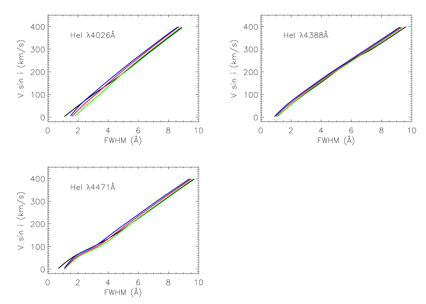
Figure 4: Calibration of synthetic FWHM versus stellar projected roational velocity for sample He i lines specified in the figure. The calculations of synthetic He i profiles adopted model atmospheres with $T_{\rm eff}$= 15,000K (black curve); $T_{\rm eff}$=20,000K (green curve) $T_{\rm eff}$=25,000K (red curve) and $T_{\rm eff}$=30,000K (blue curve). The calculations adopted an instrumental broadening corresponding to R=50,000.

The synthetic FWHM of the He i line profiles for the 4 grid effective temperatures are listed in Table 2. In Figure  4 we show the variation of these theoretical FWHM as a function of $v\sin i$; all calculations presented in this figure adopted R=50,000 as the broadening of the instrumental profile because this value corresponds roughly to the resolution of our data. We note that whilst the curves for $T_{\rm eff}$=20,000, 25,000, and 30,000 K (green, red and blue curves, respectively) run nearly paralell to each other, the black curve for $T_{\rm eff}$=15,000 K presents a different behaviour as this curve crosses the curves for the higher temperatures. This effect probably results from the fact that, for the three He i lines studied here, the line intensity as a function of spectral type reaches its maximum for B2V (Didelon, 1982), which corresponds to roughly an effective temperature of $\sim$20,000 K.

For the sake of completeness, we also calculated results for R=10,000. As expected, diagrams of $v\sin i$ versus FWHM calculated for an instrumental resolution of R=10,000 are very similar to the ones for R=50,000, with significant differences appearing only for $v\sin i$$\leq$50 ${\rm kms}^{-1}$. For a higher $v\sin i$, the rotational broadening becomes more important than the instrumental broadening and dominates the line profile. Thus, for moderate to high rotation, the $v\sin i$ values derived from the medium- and high-resolution calibrations are virtually the same. For example, considering $T_{\rm eff}$=25,000 K and a measured FWHM of 2 Å for the line 4026Å, one would obtain $v\sin i$ of 17 and 31 ${\rm kms}^{-1}$ for R=10,000 and 50,000, respectively. For a measured FWHM$\sim$3 Å, the derived $v\sin i$  from both calibrations is $\sim$90 ${\rm kms}^{-1}$.

It should be noted that our calculations ignore the flattening of the stellar photosphere and gravitational darkening, which is a flux reduction toward the equator due to the decrease of the local $T_{\rm eff}$ from the pole to the equator. These mechanisms were carefully re-analysed recently by Townsend, Owocki, & Howarth (2004) and Frémat et al. (2005), among others. For instance, Table 2 of the Townsend, Owocki, & Howarth (2004) paper shows that for $i=90^{\arcdeg}$ and $ve/vc=0.95$, where $ve$ is the equatorial rotational velocity and $vc$ is the velocity at which centrifugal forces balance Newtonian gravity at the equator, $v\sin i$ determinations that neglect these effects can be underestimated by 12 to 33% (depending on the spectral type) when the He i $\lambda$4471Å line is used. These effects rapidly become negligible as the rotational rate decreases, and only three of the stars in our sample have projected rotational velocities that exceed 300 ${\rm kms}^{-1}$ or equivalently about three-quarters of the critical velocity in the mass range surveyed here. Therefore, the effects of gravity darkening and flattening of the photosphere should be neglible for the vast majority of stars in our sample. While one should not employ our calibration for a sample of very rapidly rotating stars, such as Be-type stars, it can be safely used in a sample of OB stars like the one analyzed in this study.

One interesting application of the gravity darkening effect is the analysis of widhts of lines formed at different temperatures and thus in different latitudes over the stellar disk. As a result, the lines produced by ions with higher ionization potentials tend to form closer to the poles (Frémat et al., 2004). In practice, the lines formed in different latitudes, implying in different inclination angles $i$, present different widths, for the same $v\sin i$ value. An example of such analysis can be found in Stoeckley & Buscombe (1987), who compared He i $\lambda$4471Å to Mg ii $\lambda$4481Å and derived both $v\sin i$ and the inclination angle for a sample of 19 rapidly rotating B stars. The He lines selected for the present study, however, do not allow a similar analysis once they all present similar ionization potentials and thus probably formed over a narrow range of latitutes.

The values of $v\sin i$ achieved with our calibration, as well as a comparison among both metods and also with previous results from the literature (whenever possible) are in the next section.

5 $v\sin i$ Results

The FWHM of the three studied He i lines were measured in the same way as the theoretical He i profiles in all target star spectra. The stellar $v\sin i$ values obtained using the calibration discussed in this study are presented in Table 1: we list the sample stars with their respective clusters or associations in the first two columns and their estimated effective temperatures in column 3 (from Daflon & Cunha 2004 and references therein). The $v\sin i$’s derived from the synthesis of metal lines are listed in column 4. Columns 5-10 give the FWHM’s measured from the observed He i lines plus the respective $v\sin i$ derived using the He i calibration; and in column 11 we list the average $v\sin i$ for each star $<V\sin i_{He}>$ with the dispersions, which were computed from the individual He i lines measurements.

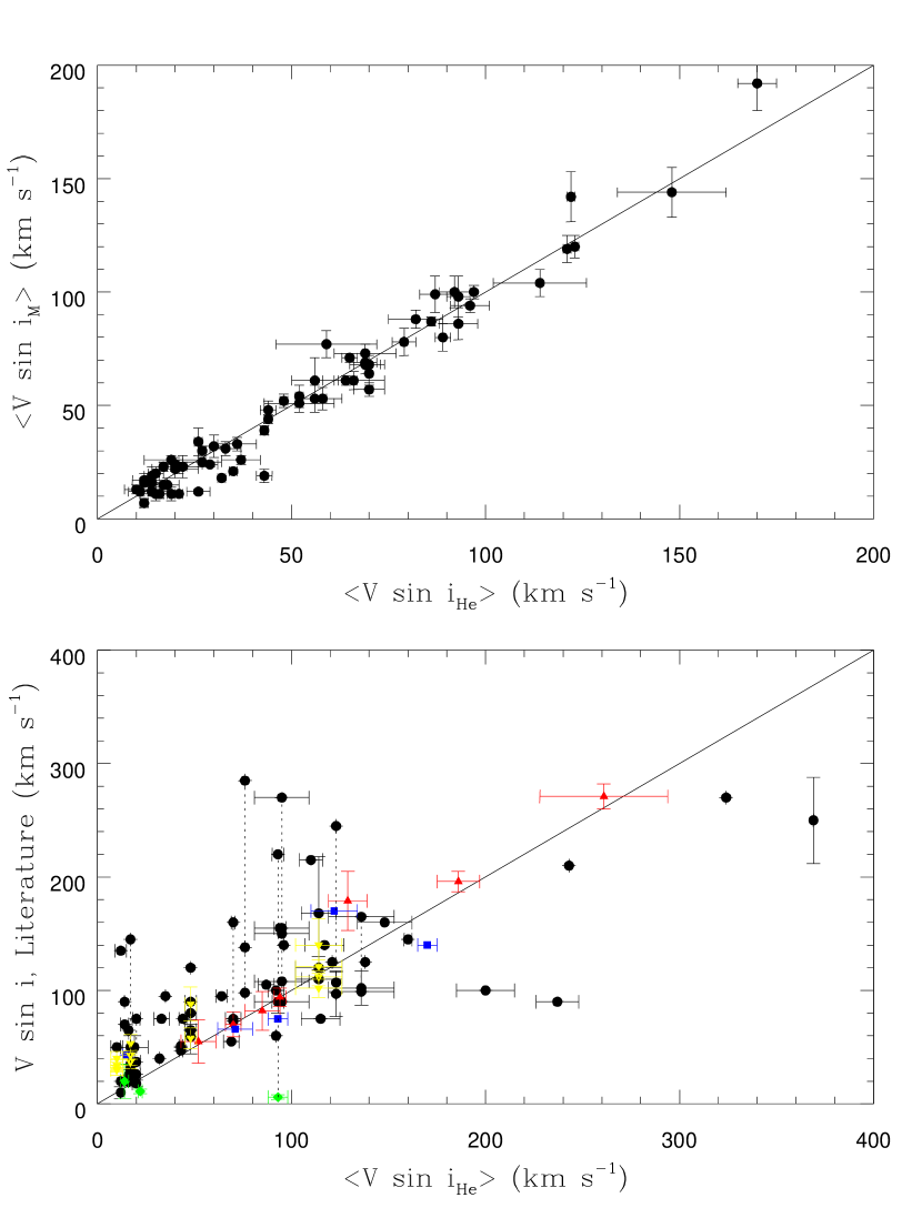
Figure 5: Top: Comparison between $v\sin i$ derived from metal and He i lines. Bottom: Comparison between mean $v\sin i$ from He i lines and values from the literature. Black crosses are for Glebocki & Stawikowski (2000); green diamonds, Gummersbach et al. (1998); red triangles, Huang & Gies (2006a); blue squares, Dufton et al. (2006); and yellow upsidedown triangles, Simón-Díaz & Herrero (2007).

A comparison of the $v\sin i$’s obtained with the two methods discussed in this paper (from synthesis of weak metal lines and using the calibration of synthetic FWHM of He i lines) is shown for the sharp lined star sample in the top panel of Figure 5. The $v\sin i$ values are in excellent agreement with no systematic differences between the two sets of results: the mean difference between $<v\sin i_{M}>$ and $<v\sin i_{He}>$ is $-0.4\pm 7.7$ ${\rm kms}^{-1}$. Considering each He i line separetely, the worst agreement with $<v\sin i_{M}>$ is found for the He i line at 4026Å, which deviates from $<V\sin i_{M}>$ by roughly +3 ${\rm kms}^{-1}$. This result might perhaps suggest that is preferable to use only the He i lines at 4388Å  and at 4471Å  in $v\sin i$ estimates. Another recent study also evaluated the differences between $v\sin i$’s obtained from the metal lines and He i profiles. Simón-Díaz & Herrero (2007) used the Fourier method and FWHM of metal and helium lines in order to determine $v\sin i$ and found that the widths of He lines tend to produce higher $v\sin i$ values than the metal lines by a factor of 10-20%. Our methods for deriving $v\sin i$, however, yield good agreement between the different indicators.

A comparison with other $v\sin i$ results from the literature is shown in the bottom panel of Figure 5. The different studies from the literature use different methods to obtain $v\sin i$ and these probably have different levels of accuracy. The $v\sin i$ values from the Fourier method and FWHM by Simón-Díaz & Herrero (2007, yellow upsidedown triangles) are on average slightly higher than ours, with a mean difference of the order of 18 ${\rm kms}^{-1}$. Gummersbach et al. (1998; green diamonds) did an abundance analysis for a sample of sharp lined stars and we have 3 stars in common with that study: the comparison with our results is good for two stars, but for BD$-$13°4921, we found $<v\sin i_{M}>=86\pm 7$ ${\rm kms}^{-1}$ and $<V\sin i_{He}>=93\pm 5$${\rm kms}^{-1}$ and they find $v\sin i$= 6 ${\rm kms}^{-1}$. Dufton et al. (2006, blue squares) also analyzed this star and found $v\sin i$= 75 ${\rm kms}^{-1}$. Other stars in Dufton et al.’s study are also in good agreement with our results. A comparison with the results from Huang & Gies (2006; red triangles), who analyzed the same He i lines as here, also indicates good agreement: $<$This study $-$ Huang & Gies $>$ = 10.0 $\pm$ 18.3 ${\rm kms}^{-1}$. Many stars in our sample have $v\sin i$ values in the recent compilation by Glebocki & Stawikowski (2000); these stars are represented as black crosses in the bottom panel of Figure 5. Since some sample stars have multiple entries in the Glebocki & Stawikowski catalogue, the different $v\sin i$ estimates in each case are connected by the dashed vertical lines in the figure. It is clear that the different values in the catalogue are sometimes quite discrepant: for example, for HD101436 the catalogue lists $v\sin i$=98 , 138 and 235 ${\rm kms}^{-1}$  and we find a $v\sin i$ value of 76 ${\rm kms}^{-1}$. In general, the $v\sin i$ results from the studies based on profile fitting agree reasonably well with our $v\sin i$ determinations while the most discrepant points in the figure are from the the compilation of Glebocki & Stawikowski, including results obtained with different methods and from spectra of different resolutions, which probably lead to the large scatter in the multiple results for a given star.

The uncertainties in the $v\sin i$ values derived from the He i lines can be estimated by considering the errors in the measurements of FWHM and from evaluating the effects of variations in the adopted effective temperature. In order to estimate the uncertainties in the $v\sin i$’s, we varied each parameter while keeping the other constant. For a given $T_{\rm eff}$=25,000K and a FWHM=6 Å, the changes in $v\sin i$  resulting from variations of 10% in the measured full-width at half maximum are similar for the three studied He i lines: about 10-12%. Considering FWHM=4 Å and changing $T_{\rm eff}$ from 20,000 to 25,000K, we found that the obtained $v\sin i$’s are increased by 11%, 3% and 8%, for the 3 He i lines, respectively.

The helium profiles are sensitive to surface gravity, being broader for larger values of $\log g$. Since our calibration was derived for a fixed $\log g$=4.0, we studied the effects of different $\log g$ values for a given $T_{\rm eff}$=25,000K. We computed profiles for a complementary grid with $\log g$=3.5 and 4.5 and measured their FWHM consistently. Considering a FWHM=$\sim$3Å, the differences among $v\sin i$ values obtained from profiles with $\log g=4.0\pm 0.3$ dex are negligible and reach 10–15% for $\delta\log g=0.5$ dex. This result suggests that our calibration can be safely used for main sequence stars with $\log g$=3.7–4.3. We note, however, that for the sharpest He lines the effect of gravity on the determination of $v\sin i$ may be larger, especially for the line 4026Å: for this line, in the worst case, the derived $v\sin i$’s can differ $\sim$50% for $\delta\log g=0.5$ dex. Thus, the use of our calibration results for stars with very sharp lines and gravities outside the range 3.7 $<\log g<$ 4.3 is not recomended.

6 Discussion

6.1 The Sample $v\sin i$ Distribution

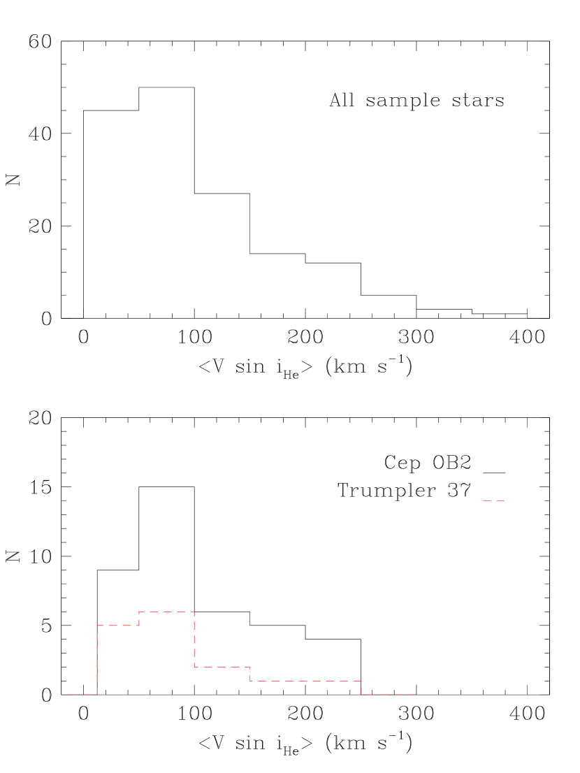
Figure 6: Top: The distributions of $v\sin i$ values for our sample. The $v\sin i$’s were obtained with a calibration of synthetic FWHM of He i lines versus stellar projected rotational velocities. Bottom: Distribution of $v\sin i$ for the 40 stars in Cep OB2 association (black histogram) and the open cluster Tr 37 (red histogram).

The histogram with the $v\sin i$ distribution for the sample of OB stars studied in this paper (belonging to a variety of clusters and associations) is shown in the top panel of Figure 6. The $v\sin i$’s shown in the histogram were all obtained from the He i lines. It is important to note, however, that the main purpose for the observed sample analyzed here was to construct an abundance database for the study of metallicity gradients in the Milky Way disk. In this context, Daflon & Cunha (2004) tried to maximize the number of targets with sharp lines, as much as possible, by conducting searches in $v\sin i$ catalogues for OB stars with low values of rotational projected velocities before the observing runs. Our observed sample is therefore not representative of a randomly selected sample of OB stars in clusters and associations and is biased by having a larger number of stars with small projected rotational velocities. Even so, the average $v\sin i$ for our whole sample of 101$\pm$76 ${\rm kms}^{-1}$is only slightly lower (but still consistent within the standard deviations) than the mean $v\sin i$ obtained by Abt, Levato & Grosso (2002) for a sample of main sequence B0-B2 stars: 127$\pm$8 ${\rm kms}^{-1}$. This agreement is probably the result of the fact that the the latter sample included mainly field stars and members of unbound associations, two groups that also contain large numbers of slowly rotating stars (Wolff et al., 2007).

6.2 The Cep OB2 Association

The Cep OB2 association merits a separate discussion in this study because the observations conducted for this association are fairly complete down to magnitude V=10 and are without any bias in the selection of targets. We observed 40 targets between spectral types O9-B3 representing all the main-sequence stars (within these spectral types) listed in Garmany & Stencel (1992). Two stars have been discarded from our sample due to the very high $T_{\rm eff}$ ($>\sim$35,000K) obtained. The lines for two double-lined spectroscopic binaries (HD 208905 and HD 239738) could be resolved, resulting in $v\sin i$ determinations for the two components in each system, which were considered separately. Three B stars out of our original list are not included in Table 1 because a defect in the detector prevented measurement of He i 4471 Å and the measurements of the He i 4388 Å are rather uncertain, due to bad quality data. (The He line at 4026Å is not covered in the spectra of the northern sample). In order to have a complete sample for comparison with data in the literature on other clusters and associations we have estimated approximate $v\sin i$ values from He i 4388 Å as follows: HD 204827, 102 ${\rm kms}^{-1}$; HD 206081, 245 ${\rm kms}^{-1}$; HD 239869, 229 ${\rm kms}^{-1}$. Our final sample thus comprises 40 stars: 16 stars belong to the youngest cluster Trumpler 37, the nucleus of the OB association (with an age of 11 Myr, Dias et al. 2002) and 24 stars are from a larger area which includes the more sparse cluster NGC 7160 (with an age of 19 Myr, Dias et al. 2002).

The histograms in the bottom panel of Figure 6 show the $v\sin i$ distributions of the stars in the Cep OB2 association (represented by the black histogram) and in Tr 37 (represented by the red histogram). The two distributions are not significantly different, especially given the small number of stars in each sample.

A recent paper has presented evidence that the $v\sin i$ distribution in clusters depends on the environment in which the stars formed, with the differences being much larger at low velocities. The sense of the difference is that a larger fraction of stars with low rotation are found in low density regions as compared with stars formed in high density regions (Wolff et al., 2007). The proportion of slow rotators among field stars is still higher.

If we assume that Cep OB2 occupies the region within l=96 – 108$\arcdeg$ and b=$-$1 – +12$\arcdeg$ with a distance from the Sun of 615 pc (de Zeeuw et al., 1999), the median radius of the association is 64 pc. The total mass of stars earlier than B3 is $4\times 10^{3}M_{\sun}$ (Simonson, 1968) and the stellar density in Cep OB2 is thus 0.02 $M_{\sun}pc^{-3}$. According to these parameters and following (Wolff et al., 2007), Cep OB2 can be classified as an unbound stellar ensemble, as already suggested by Kun (1986). Figure 7 compares the cumulative distribution of $v\sin i$ for all of the stars in Cep OB2, Trumpler 37, and NGC 7160 combined with the distributions for stars in low density, unbound associations and high density, bound clusters taken from Wolff et al. (2007). For this comparison, we have eliminated the five stars in Table 1 that are hotter than the temperature range included in the Wolff et al. survey. As the figure shows, the distribution for Cep OB2 is similar to that of the stars in low density regions. A K-S test indicates that the probability that the distributions for Cep OB2 and the open associations are drawn from the same parent sample is 0.60. For both groups, more than 20% of the stars have projected rotational velocities that are less than 50 ${\rm kms}^{-1}$ and about 50% have apparent rotational velocities less than 100 ${\rm kms}^{-1}$. However, a K-S test shows that there is also a 9% probability that the distribution for Cep OB2 is drawn from the same parent sample as the bound clusters in Fig. 7. Given the large intrinsic spread in the distribution of $v\sin i$ in any group of B stars, a sample even as large as we have observed in Cep OB2 is not enough to make a definitive test of a potential relationship between environment and rotation. (The probability that the distributions for the stars in low and high density regions shown in Fig. 7 are drawn from the same parent population is only 0.001. The difference between these two groups is more significant than the difference between Cep OB2 and the high density group because of the much larger sample size of the stars in low density regions–141 stars in low density regions and only 35 stars in Cep OB2.)

6.3 Summary and Conclusions

We present $v\sin i$ values for a sample of 156 main sequence OB stars in the Galactic disk. The $v\sin i$’s were derived from a calibration for the FWHM of theoretical profiles of He i lines at $\lambda\lambda$4026, 4388, and 4471 Å as a function of the stellar rotation. For a subsample of 69 sharp-lined stars, we also derived $v\sin i$ from non-LTE synthesis of metal lines. The $v\sin i$ values obtained from metal and helium lines show good agreement, and the values we derive are in good agreement with published rotational velocities. Thus, we conclude that our calibration is an useful and rapid tool for estimating the projected rotational velocities for O9 to B5 main-sequence stars that are rotating at $v\sin i$ up to about 300${\rm kms}^{-1}$. For most of the stars in this study, our distribution of $v\sin i$ is biased toward low $v\sin i$ and is not representative for main sequence B stars sampled randomly. This effect is related to the selection criteria originally imposed in order to study abundance gradients in the Galactic disk. The one exception is the association, Cep OB2, where all the main sequence stars earlier than B3 were observed. The distribution of $v\sin i$ for this unbound association is consistent with the distribution for stars in other unbound associations studied by Wolff et al. (2007), thereby adding support for the hypothesis that the distribution of rotational velocities for early B stars depends on the environment in which they formed.

Figure 1: Observed profiles of He i lines at $\lambda\lambda$4026, 4388 and 4471 Å for star Sh2-47 3.

Figure 2: Comparison between observed and non-LTE synthetic profiles for one of the spectral regions containing the O ii line at 4943 Å. The observed spectrum is for the target star Sh 2-47 3 and the synthetic profiles were calculated for different sets of parameters. Top: on the left panel we show synthetic profiles calculated for five values of oxygen abundances (indicated in the figure). The best fit oxygen abundance is derived for $\log\epsilon(O)$=8.45 (represented by the solid line). In the right panel we present the variation of $\chi^{2}$ as a function of oxygen abundance. Bottom: same for different values of $v\sin i$ varying from 5.5 to 25.5 ${\rm kms}^{-1}$.

Figure 3: Theoretical profiles non-convolved for rotation of He i lines at $\lambda\lambda$4026, 4388 and 4471Å, computed for $T_{\rm eff}=$25,000 K, $\log g$=4.0 and $\xi$=5.0 ${\rm kms}^{-1}$.

Figure 7: Comparison of the cumulative distribution of $v\sin i$ for 35 B stars in Cep OB2 (filled circles) with the distribution for 141 stars in low density regions (crosses) and 268 stars in high density regions (triangles). The distribution of $v\sin i$ for the stars in Cep OB2 is more similar to the distribution of stars formed in low density regions but the distinction is only marginally significant because of the relatively small number of stars in Cep OB2.

Table 1: $V\sin i$ Results

Cluster	Star	$T_{\rm eff}$	$<V\sin i_{M}>$	W4026	$V\sin i_{4026}$	W4387	$V\sin i_{4387}$	W4471	$V\sin i_{4471}$	$<V\sin i_{He}>$
		(K)	(km s-1)		(km s-1)		(km s-1)		(km s-1)	(km s-1)
Ara OB1	HD 149065	21540	24$\pm$1	$\cdots$	$\cdots$	1.5	31	1.5	28	29$\pm$2
	HD 153106	25510	$\cdots$	4.5	180	4.0	163	4.5:	161	168$\pm$10
Cen OB1	HD 100368	22000	$\cdots$	$\cdots$	$\cdots$	1.2:	14	1.2:	9	11$\pm$4
	HD 101794	23970	$\cdots$	5.4	227	5.7	231	5.5	207	224$\pm$15
	HD 102415	30290	$\cdots$	7.0:	318	$\cdots$	$\cdots$	7.6	317	318$\pm$1
	HD 102463	20000	$\cdots$	2.8	65	2.3	72	2.7	78	72$\pm$6
Cep OB2	HD 203374	30000	$\cdots$	$\cdots$	$\cdots$	5.5:	234	$\cdots$	$\cdots$	234
	HD 204150	26450	$\cdots$	$\cdots$	$\cdots$	3.6	145	4.2	147	146$\pm$2
	HD 205794	26890	12$\pm$2	$\cdots$	$\cdots$	1.4	16	1.2	12	14$\pm$3
	HD 205948	24350	144$\pm$11	$\cdots$	$\cdots$	3.9	157	4.1	138	148$\pm$14
	HD 206183	33310	16$\pm$2	$\cdots$	$\cdots$	1.0	12	$\cdots$	$\cdots$	12
	HD 206267A	33330	$\cdots$	$\cdots$	$\cdots$	2.7:	105	2.6:	85	95$\pm$14
	HD 206267C	26760	$\cdots$	$\cdots$	$\cdots$	4.2	174	4.8	178	176$\pm$3
	HD 206267D	26100	44$\pm$2	$\cdots$	$\cdots$	1.6	43	1.7	45	44$\pm$1
	HD 206327	21900	15$\pm$3	$\cdots$	$\cdots$	1.3	20	1.3	15	18$\pm$3
	HD 207017	19410	$\cdots$	$\cdots$	$\cdots$	4.8	194	4.8	167	181$\pm$19
	HD 207308	23250	$\cdots$	$\cdots$	$\cdots$	4.8:	198	5.7	216	207$\pm$13
	HD 207538	32190	39$\pm$2	$\cdots$	$\cdots$	1.5	42	1.6	44	43$\pm$1
	HD 207951	20650	87$\pm$2	$\cdots$	$\cdots$	2.5	86	$\cdots$	$\cdots$	86
	HD 208266	24840	$\cdots$	$\cdots$	$\cdots$	3.2:	124	3.5:	110	117$\pm$10
	HD 208440	26470	$\cdots$	$\cdots$	$\cdots$	2.5	92	3.1	96	94$\pm$3
	HD 208905a	27460	$\cdots$	$\cdots$	$\cdots$	1.4	33	1.6	41	37$\pm$5
	HD 208905b	27460	$\cdots$	$\cdots$	$\cdots$	1.7	54	2.0:	62	58$\pm$6
	HD 209339	31250	98$\pm$9	$\cdots$	$\cdots$	2.5	96	2.8	91	93$\pm$3
	HD 209454	25460	$\cdots$	$\cdots$	$\cdots$	4.2:	173	$\cdots$	$\cdots$	173
	HD 213023	26050	$\cdots$	$\cdots$	$\cdots$	2.5	91	3.1:	96	94$\pm$3
	HD 213757	20000	$\cdots$	$\cdots$	$\cdots$	4.1	162	4.7	159	160$\pm$2
	HD 235618	27180	100$\pm$3	$\cdots$	$\cdots$	2.6	97	3.1	97	97$\pm$0
	HD 239649	20000	$\cdots$	$\cdots$	$\cdots$	3.8	148	4.8	164	156$\pm$11
	HD 239676	24720	$\cdots$	$\cdots$	$\cdots$	2.6:	95	3.3:	102	98$\pm$5
	HD 239681	26830	142$\pm$11	$\cdots$	$\cdots$	3.1	121	3.7	123	122$\pm$1
	HD 239710	21900	64$\pm$5	$\cdots$	$\cdots$	2.2	70	2.4	70	70$\pm$0
	HD 239712	18870	$\cdots$	$\cdots$	$\cdots$	5.9:	243	$\cdots$	$\cdots$	243
	HD 239724	24790	34$\pm$6	$\cdots$	$\cdots$	1.3	26	$\cdots$	$\cdots$	26
	HD 239725	20540	$\cdots$	$\cdots$	$\cdots$	3.3	125	4.1	130	127$\pm$4
	HD 239729	28450	99$\pm$8	$\cdots$	$\cdots$	2.3	84	2.8	89	87$\pm$4
	HD 239738a	21060	$\cdots$	$\cdots$	$\cdots$	$\cdots$	$\cdots$	2.0:	54	54
	HD 239738b	21060	$\cdots$	$\cdots$	$\cdots$	2.0	58	1.9	50	54$\pm$6
	HD 239742	22470	30$\pm$2	$\cdots$	$\cdots$	1.4	27	$\cdots$	$\cdots$	27
	HD 239743	21580	17$\pm$3	$\cdots$	$\cdots$	1.2	14	1.2	10	12$\pm$3
	HD 239745	27340	61$\pm$2	$\cdots$	$\cdots$	1.9	62	2.1	66	64$\pm$3
	HD 239748	27480	68$\pm$4	$\cdots$	$\cdots$	2.0	67	2.3	73	70$\pm$4
	HD 239767	29940	$\cdots$	$\cdots$	$\cdots$	2.6:	100	$\cdots$	$\cdots$	100
Cep OB3	BD +62°2125	23480	48$\pm$4	$\cdots$	$\cdots$	1.7	45	1.7	42	44$\pm$2
	BD +62°2127	22630	$\cdots$	$\cdots$	$\cdots$	2.6	92	$\cdots$	$\cdots$	92
	HD 217657	27950	13$\pm$2	$\cdots$	$\cdots$	1.1	13	1.1	8	10$\pm$3
	HD 218342	30020	31$\pm$3	$\cdots$	$\cdots$	1.3	30	1.5	37	33$\pm$4
Cyg OB3	BD +35°3956	24840	$\cdots$	$\cdots$	$\cdots$	6.5	273	$\cdots$	$\cdots$	273
	HD 191566	27290	$\cdots$	$\cdots$	$\cdots$	2.6	96	$\cdots$	$\cdots$	96
	HD 191567	22520	$\cdots$	$\cdots$	$\cdots$	1.6	20	$\cdots$	$\cdots$	20
	HD 227460	27060	11$\pm$3	$\cdots$	$\cdots$	1.5	19	$\cdots$	$\cdots$	19
	HD 227586	27830	21$\pm$1	$\cdots$	$\cdots$	1.6	35	$\cdots$	$\cdots$	35
	HD 227621	23230	$\cdots$	$\cdots$	$\cdots$	2.8	103	$\cdots$	$\cdots$	103
	HD 227696	29100	120$\pm$5	$\cdots$	$\cdots$	3.1	123	$\cdots$	$\cdots$	123
	HD 227757	32480	26$\pm$2	$\cdots$	$\cdots$	1.3	15	1.3	24	19$\pm$7
	HD 227877	23260	$\cdots$	$\cdots$	$\cdots$	3.7	147	$\cdots$	$\cdots$	147
	HD 228199	29870	104$\pm$6	$\cdots$	$\cdots$	2.7	105	3.0	122	114$\pm$12
Cyg OB7	BD +44°3594	30620	$\cdots$	$\cdots$	$\cdots$	4.6	195	$\cdots$	$\cdots$	195
	HD 197512	23570	12$\pm$2	$\cdots$	$\cdots$	1.5	14	$\cdots$	$\cdots$	14
	HD 198931	23410	$\cdots$	$\cdots$	$\cdots$	8.7:	369	$\cdots$	$\cdots$	369
	HD 199579	32930	$\cdots$	$\cdots$	$\cdots$	2.0	70	2.1	69	70$\pm$1
	HD 201666	19900	$\cdots$	$\cdots$	$\cdots$	3.6	138	$\cdots$	$\cdots$	138
	HD 202163	18560	$\cdots$	$\cdots$	$\cdots$	4.7	189	$\cdots$	$\cdots$	189
	HD 202253	22750	52$\pm$3	$\cdots$	$\cdots$	1.8:	48	$\cdots$	$\cdots$	48
	HD 202347	23280	119$\pm$6	$\cdots$	$\cdots$	3.2	121	$\cdots$	$\cdots$	121
IC 2944	HD 101070	29550	$\cdots$	2.7	87	2.1	75	2.9:	92	85$\pm$9
	HD 101084	26750	$\cdots$	3.7	136	$\cdots$	$\cdots$	3.7	123	129$\pm$10
	HD 101223	30800	$\cdots$	2.4:	71	1.9	65	2.2	73	70$\pm$4
	HD 101413	28430	$\cdots$	3.4	124	3.6	148	$\cdots$	$\cdots$	136$\pm$17
	HD 101436	33270	$\cdots$	$\cdots$	$\cdots$	$\cdots$	$\cdots$	2.3:	76	76
	HD 308810	26400	51$\pm$4	2.1	43	1.8	54	2.0	60	52$\pm$9
	HD 308813	33320	$\cdots$	4.4	183	4.2	177	5.1	198	186$\pm$11
	HD 308817	22940	57$\pm$3	2.7	68	2.1	66	2.5	74	70$\pm$4
	HD 308833	23340	$\cdots$	6.5	284	5.7:	237	$\cdots$	$\cdots$	261$\pm$33
Lac OB1	HD 214167	26720	18$\pm$1	$\cdots$	$\cdots$	1.4	32	$\cdots$	$\cdots$	32
	HD 214680	33690	23$\pm$2	$\cdots$	$\cdots$	1.1	17	$\cdots$	$\cdots$	17
	HD 216916	23520	11$\pm$2	$\cdots$	$\cdots$	1.2	16	$\cdots$	$\cdots$	16
	HD 217227	19000	15$\pm$2	$\cdots$	$\cdots$	1.3	17	$\cdots$	$\cdots$	17
	HD 217811	19070	7$\pm$2	$\cdots$	$\cdots$	1.2	12	$\cdots$	$\cdots$	12
	HD 218674	18840	$\cdots$	$\cdots$	$\cdots$	7.8	324	$\cdots$	$\cdots$	324
Mon OB2	HD 46106	29150	$\cdots$	3.2:	114	2.7	104	3.6:	122	114$\pm$9
	HD 46202	31500	24$\pm$3	$\cdots$	$\cdots$	1.1	19	1.3	22	20$\pm$2
	HD 46966	30230	$\cdots$	2.0	44	1.6	48	1.7	51	48$\pm$3
	HD 47360	26250	$\cdots$	5.3	226	5.6	237	6.3	248	237$\pm$11
	HD 47417	31550	$\cdots$	3.4	128	3.2	129	3.7	129	129$\pm$1
	HD 259105	27750	$\cdots$	4.6	190	4.5	188	5.0	190	189$\pm$1
NGC 1893	S2R2N43	24020	54$\pm$5	$\cdots$	$\cdots$	1.8	52	$\cdots$	$\cdots$	52
	S2R3N09	26160	11$\pm$3	$\cdots$	$\cdots$	1.2	18	1.2	13	15$\pm$4
NGC 2414	LS 400	30000	$\cdots$	5.0	216	5.3	226	5.4	213	218$\pm$7
	LS 404	23260	32$\pm$5	2.0	26	1.5	33	1.5	25	30$\pm$4
	LS 427a	28790	$\cdots$	3.4	124	3.2	128	3.6:	121	125$\pm$3
	LS 427b	28790	$\cdots$	3.8	147	3.6	147	4.0:	142	145$\pm$3
	LS 428	28140	33$\pm$3	1.9	32	1.4	34	1.6	42	36$\pm$5
	LS 531	26070	$\cdots$	4.5	181	4.5	181	4.8	177	181$\pm$5
NGC 2439	CD -32°4257a	28560	$\cdots$	$\cdots$	$\cdots$	5.0	212	5.5	215	213$\pm$3
	CD -32°4257b	28560	$\cdots$	$\cdots$	$\cdots$	6.2	264	6.5	263	263$\pm$1
	CPD -33°1682	33210	$\cdots$	2.3	64	2.0:	70	2.0	65	67$\pm$3
	HD 61851	28060	$\cdots$	4.0:	157	3.7:	151	4.1	145	151$\pm$5
	LS 709	31410	$\cdots$	4.5	191	4.8	204	5.8	231	209$\pm$20
NGC 3576	HD 97499	28590	$\cdots$	4.9	208	4.8	203	5.0:	191	201$\pm$8
NGC 4755	CPD -59°4532	23610	71$\pm$2	2.6	64	2.1	67	2.2	65	65$\pm$2
	CPD -59°4535	22930	68$\pm$4	2.7	68	2.1	66	2.5	74	69$\pm$4
	CPD -59°4544	24330	69$\pm$5	2.6	66	2.1	68	2.4	72	69$\pm$3
	CPD -59°4557	23240	$\cdots$	3.7	127	2.9	108	4.0	131	122$\pm$12
	CPD -59°4560	22390	192$\pm$12	4.5	172	4.4	174	4.7	164	170$\pm$5
NGC 6031	NGC 6031 12	19050	$\cdots$	1.9	17	$\cdots$	$\cdots$	1.4	24	21$\pm$5
	NGC 6031 40	19010:	$\cdots$	3.5	108	$\cdots$	$\cdots$	3.3	98	103$\pm$6
	NGC 6031 74	21600:	$\cdots$	2.2:	34	$\cdots$	$\cdots$	1.6	34	34$\pm$0
NGC 6204	CPD -46°8206	15000:	$\cdots$	1.8:	39	1.3:	22	1.1:	26	29$\pm$9
	HD 150627	29620	$\cdots$	3.8	149	3.6	148	4.0	143	147$\pm$3
	LS 3719	24120	77$\pm$6	2.3	50	1.8	52	2.5	74	59$\pm$13
NGC 6604	BD -12°4978	27750	61$\pm$4	2.3	58	2.0	68	2.3	73	66$\pm$8
NGC 6611	BD -12°5074	26210	19$\pm$3	2.1	41	1.6	43	1.7	45	43$\pm$2
	BD -13°4921	29540	86$\pm$7	$\cdots$	$\cdots$	2.4	90	3.0	97	93$\pm$5
	BD -13°4929	30600	$\cdots$	2.6:	80	2.0	70	1.9	62	71$\pm$9
	BD -13°4930	30830	20$\pm$3	$\cdots$	$\cdots$	1.1	17	1.2	13	15$\pm$2
	BD -13°4934	30970	80$\pm$6	$\cdots$	$\cdots$	2.4	91	2.7	88	89$\pm$2
	HD 170452	29890	$\cdots$	3.2:	116	$\cdots$	$\cdots$	3.4	114	115$\pm$2
NGC 6231	CPD -41°7723	24920	26$\pm$2	2.1	37	1.6	42	1.5	31	37$\pm$5
	CPD -41°7730	24670	12$\pm$1	1.9	23	1.4	30	1.4	24	26$\pm$3
	HD 326332	27030	23$\pm$3	1.7	21	1.2	20	1.4	27	21$\pm$5
	HD 326364	29610	19$\pm$4	1.6	13	1.1	16	1.2	13	14$\pm$2
Pismis 20	Pismis 20 6	27650	$\cdots$	$\cdots$	$\cdots$	$\cdots$	$\cdots$	2.4	76	76
R 105	HD 144900	27340	$\cdots$	3.0:	103	2.9:	112	3.5:	114	110$\pm$6
	HD 144970	30760	$\cdots$	3.2	116	3.1	125	3.2	105	115$\pm$10
R 103	CPD -50°9216	20040	$\cdots$	$\cdots$	$\cdots$	5.6	230	$\cdots$	$\cdots$	230
Sct OB2	BD -08°4617	31410	$\cdots$	3.1	111	2.8	110	2.9	95	105$\pm$9
	BD -08°4634	29360	$\cdots$	2.4	69	2.2	80	2.5	82	77$\pm$7
	HD 172367	28640	$\cdots$	5.3:	229	5.7	242	6.2:	249	240$\pm$10
	HD 172427	26360	53$\pm$5	2.3	52	1.9	60	2.0	60	58$\pm$5
	HD 172488	26530	100$\pm$7	2.9	89	2.6	97	2.9	90	92$\pm$4
	HD 173637	31950	$\cdots$	4.5	190	5.0	211	$\cdots$	$\cdots$	200$\pm$15
Sh 2-16	LS 4381	22500	$\cdots$	3.3:	100	$\cdots$	$\cdots$	2.9	86	93$\pm$10
Sh 2-29	HD 166192	28010	$\cdots$	3.7	139	3.2:	127	3.5:	115	127$\pm$12
Sh 2-32	HD 166033	27290	73$\pm$4	2.4	63	2.0	67	2.5	78	69$\pm$8
	HD 314031	27650	94$\pm$3	2.9	93	2.5	93	3.2	102	96$\pm$5
Sh 2-47	Sh 2-47 3	29870	16$\pm$2	1.6	13	1.1	16	1.2	13	14$\pm$2
Sh 2-247	Sh 2-247 1	31560	23$\pm$5	1.7	22	1.2	23	1.3	22	22$\pm$1
Sh 2-253	LS 45	22830	22$\pm$4	$\cdots$	$\cdots$	1.4	25	1.3	16	20$\pm$6
	LS 51	32630	$\cdots$	6.1	273	6.6:	282	7.9:	275	277$\pm$5
Sh 2-284	HD 48691	27870	53$\pm$6	2.2	52	1.8	57	1.9	58	56$\pm$3
Sh 2-285	BD -00°1491	29480	12$\pm$2	$\cdots$	$\cdots$	1.0	9	1.2	13	11$\pm$3
Sh 2-289	Sh 2-289 2	25060	$\cdots$	$\cdots$	$\cdots$	2.3	80	2.4	74	76$\pm$5
	Sh 2-289 4	24560	$\cdots$	$\cdots$	$\cdots$	2.2	74	1.2	58	66$\pm$11
Sh 2-301	LS 212	21980	$\cdots$	5.0	200	5.9	245	5.7	214	219$\pm$23
Stock 16	CPD -61°3576	29100	$\cdots$	2.6:	80	2.3:	85	2.9:	93	86$\pm$7
	CPD -61°3579	27840	78$\pm$6	2.6	76	2.2	78	2.6	83	79$\pm$3
	CPD -61°3581	25810	$\cdots$	5.9:	257	6.3:	266	6.9:	279	267$\pm$11
Tr 27	LS 4257	29460	88$\pm$4	2.5	76	2.2	80	2.8	89	82$\pm$7
	LS 4264	22360	$\cdots$	3.1	88	2.9:	107	3.7:	115	103$\pm$13
	LS 4271	32190	61$\pm$10	2.1	51	1.7	54	2.0	64	56$\pm$6
Vul OB1	BD +24°3880	30410	11$\pm$1	$\cdots$	$\cdots$	1.1	21	$\cdots$	$\cdots$	21
	BD +24°3843	23250	$\cdots$	$\cdots$	$\cdots$	4.1	166	3.4	131	148$\pm$25
	HD 344783	31010	25$\pm$2	1.7	22	1.3	30	1.4	30	27$\pm$5
	NGC 6823 Hoag6	31550	$\cdots$	$\cdots$	$\cdots$	2.2	81	2.6	85	83$\pm$3
…	RL 41	20350	$\cdots$	$\cdots$	$\cdots$	2.9	104	3.3	96	100$\pm$6

Table 2: Full-Widths at Half Maximum of theoretical He profiles (in Å), for R=50,000

V $\sin i$	4026Å	4388Å	4471Å	4026Å	4388Å	4471Å
(km s-1)
		$T_{\rm eff}$=15,000 K			$T_{\rm eff}$=20,000 K
0	1.04	1.02	0.65	1.74	0.99	1.09
50	2.01	1.90	1.59	2.54	1.89	1.93
100	3.01	2.86	3.03	3.43	2.82	3.42
150	4.10	3.92	4.38	4.25	3.84	4.53
200	5.11	4.94	5.49	5.08	4.92	5.49
250	6.05	6.02	6.55	5.98	6.07	6.51
300	7.01	7.34	7.61	6.92	7.22	7.55
350	7.99	8.51	8.66	7.90	8.36	8.60
400	8.99	9.64	9.77	8.87	9.48	9.68
		$T_{\rm eff}$=25,000 K			$T_{\rm eff}$=30,000 K
0	1.55	0.91	1.06	1.44	0.86	1.05
50	2.30	1.74	1.82	2.08	1.63	1.69
100	3.16	2.70	3.25	2.91	2.59	3.07
150	4.01	3.73	4.31	3.80	3.63	4.11
200	4.87	4.81	5.31	4.71	4.71	5.13
250	5.79	5.95	6.33	5.65	5.86	6.18
300	6.74	7.12	7.37	6.63	7.00	7.22
350	7.71	8.25	8.45	7.62	8.14	8.32
400	8.71	9.36	9.54	8.65	9.27	9.42

References

- Abt, Levato & Grosso (2002) Abt, H. A., Levato, H. & Grosso, M. 2002, ApJ 573, 359
- Barnard, Cooper & Shamey (1969) Barnard, A. J., Cooper, J., & Shamey, L. J. 1969, A&A, 1, 28
- Becker & Butler (1988) Becker, S. R. & Butler, K. 1988, A&A 201, 232
- Becker & Butler (1989) Becker, S. R. & Butler, K. 1989, A&A 209, 244
- Becker & Butler (1990) Becker, S. R. & Butler, K. 1990, A&AS 84, 95
- Butler & Giddings (1985) Butler, K., & Giddings, J. R. 1985, in Newsletter on Analysis of Astronomical Spectra, No. 9 (London: Univ. London)
- Daflon, Cunha & Becker (1999) Daflon, S., Cunha, K., & Becker, S. 1999, ApJ 522, 950
- Daflon et al. (2001a) Daflon, S., Cunha, K., Becker, S., & Smith, V. V. 2001a, ApJ 552, 309
- Daflon et al. (2001b) Daflon, S., Cunha, K., Butler, K., & Smith, V. V. 2001b, ApJ 563, 325
- Daflon et al. (2003) Daflon, S., Cunha, K., Smith, V. V., & Butler, K. 2003, A&A 399, 525
- Daflon, Cunha, & Butler (2004a) Daflon, S., Cunha, K., & Butler, K. 2004a, ApJ 604, 362
- Daflon, Cunha, & Butler (2004b) Daflon, S., Cunha, K., & Butler, K. 2004b, ApJ 606, 514
- Daflon & Cunha (2004) Daflon, S. & Cunha, K. 2004, ApJ 617, 1115
- de Zeeuw et al. (1999) de Zeeuw, P. T., Hoogerwerf, R., de Bruijne, J. H. J., Brown, A. G. A. & Blaauw, A. 1999, 1999 AJ 117, 354
- Dias et al. (2002) Dias, W. S., Alessi, B. S., Moitinho, A. & Lépine, J. R. D. 2002, A&A 389, 871
- Didelon (1982) Didelon, P. 1982, A&AS 50, 199
- Dufton et al. (1986) Dufton, P. L., Brown, P. J. F., Lennon, D. J. & Lynas-Gray, A. E. 1986, MNRAS 222, 713
- Dufton et al. (2006) Dufton, P. L., Smartt, S. J., Lee, J. K., Ryans, R. S. I., Hunter, I., Evans, C. J., Herrero, A., Trundle, C., Lennon, D. J., Irwin, M. J, and Kaufer, A. 2006, A&A 457, 265
- Eber & Butler (1988) Eber, F. & Butler, K. 1988, A&A 202, 153
- Frémat et al. (2004) Frémat, Y., Zorec, J., Hubert, A.-M., Floquet, M., Leister, N., Levenhagen, R., Chauville, J., & Ballereau, D. 2003, in IAU Symp. 215, Stellar Rotation, ed. A. Maeder & P. Eenens (San Francisco:ASP), 23
- Frémat et al. (2005) Frémat, Y., Zorec, J., Hubert, A.-M., & Floquet, M. 2005, A&A 440, 305
- Garmany & Stencel (1992) Garmany, C. D. & Stencel, R. E. 1992, A&AS 94, 211
- Giddings (1981) Giddings, J. R. 1981, Ph.D. Thesis, Univ. London
- Glebocki & Stawikowski (2000) Glebocki, R. & Stawikowski, A. 2000, Acta Astronomica 50, 509
- Gummersbach et al. (1998) Gummersbach, C. A., Kaufer, A., Schaefer, D. R., Szeifert, T., & Wolf, B. 1998, A&A 338, 881
- Howarth et al. (1997) Howarth, I. D., Siebert, K. W., Hussain, G. A. J. & Prinja, R. K. 1997, MNRAS 284, 265
- Huang & Gies (2006a) Huang, W. & Gies, D. R. 2006, ApJ 648, 580
- Huang & Gies (2006b) Huang, W. & Gies, D. R. 2006, ApJ 648, 591
- Kun (1986) Kun, M. 1986, Ap&SS 125, 13
- Kurucz, (1993) Kurucz, R. L. 1993, Kurucz CD-ROM No. 13 (Cambridge, Mass.: Smithsonian Astrophysical Observatory)
- Nieva & Przybilla (2007) Nieva, M. F. & Przybilla, N. 2007, A&A 467, 295
- Przybilla et al. (2001) Przybilla, N., Butler, K., Becker, S. R. & Kudritzki, R.P. 2001, A&A
- Przybilla (2005) Przybilla, N. 2005, A&A 443, 293
- Shamey (1969) Shamey, L.J. 1969, Ph.D. Thesis, University of Colorado.
- Simón-Díaz & Herrero (2007) Simón-Díaz, S. & Herrero A. 2007, A&A 468, 1063
- Simonson (1968) Simonson, S. C. 1968, ApJ 154, 928
- Slettebak et al. (1975) Slettebak, A., Collins, G. W., II, Parkinson, T. D., Boyce, P. B., & White, N. M. 1975, ApJS 29, 137
- Slettebak (1982) Slettebak, A. 1982, ApJS 50, 55
- Stoeckley & Buscombe (1987) Stoeckley, T. R. & Buscombe, W. 1987, MNRAS 227, 801
- Townsend, Owocki, & Howarth (2004) Townsend, R. H. D., Owocki, S. P., & Howarth, I. D. 2004, MNRAS 350, 189
- Vrancken, Butler & Becker (1996) Vrancken, M., Butler, K & Becker, S. R. 1996, A&AS 311, 661
- Wade & Rucinski (1985) Wade, R. A., Rucinski, S. M. 1985, A&ASS, 60, 471
- Wolff et al. (2007) Wolff, S. C., Strom, S. E., Dror, D. & Venn, K. 2007, AJ 133, 1092