Branching ratio measurement of $K_{S}\rightarrow\gamma\gamma$ decay using a pure $K_{S}$ beam in the KLOE detector

Abstract

We have analyzed 1.62 fb^-1 of $e^{+}e^{-}$ collisions at a center of mass energy $\sim M_{\phi}$ collected by the KLOE experiment at DA$\Phi$NE. This sample corresponds to a production of $\sim$ 1.7 billion of $K_{S}$ $K_{L}$ pairs which allowed us to search for the rare $K_{S}\to\gamma\gamma$ decay. $K_{S}$ are tagged by the $K_{L}$ interaction in the calorimeter and the signal is searched for by requiring two additional prompt photons. Strong kinematic requirements reduce the initial 0.5$\times 10^{6}$ events to 2300 candidates from which we extract a signal of 600 $\pm$ 35 events. By normalizing to the $\mbox{$K_{S}$}\ \to 2\pi^{0}$ decays counted in the same sample, the measured value of BR($\mbox{$K_{S}$}\to\gamma\gamma$) is (2.27 $\pm 0.13(stat.)^{+0.03}_{-0.04}(syst.))\times 10^{-6}$, in agreement with $O(P^{4})$ Chiral Perturbation Theory predictions.

, , , , , , , , , , , , , , , , , , , , , , , , , , , , , , , , , , , , , , , , , , , , , , , , , , , , , , , , , , , , , , , , , , , , , , , , , , , , , , , , ,

1 Introduction

A precise measurement of the $K_{S}\to\gamma\gamma$ decay rate is an important test of Chiral Perturbation Theory ($\chi PT$) predictions. The decay amplitude of $K_{S}\to\gamma\gamma$ has been evaluated at the leading order of $\chi PT$ [1], $O(P^{4})$, providing the estimate of the corresponding branching ratio, $BR(KS\rightarrow\gamma\gamma)=2.1\times 10^{-6}$, with a few percent precision. This result is in agreement with the experimental measurement of NA31, that obtained $BR(K_{S}\rightarrow\gamma\gamma)=(2.4\pm 0.9)\times 10^{-6}$ [2]. The last precise determination of this $BR(K_{S}\rightarrow\gamma\gamma)$ of $2.71\times 10^{-6}$, with a total uncertainty below 3%, comes from NA48 [3]. The last mentioned result differs from $\chi PT$ $O(P^{4})$ prediction of about 30%, indicating possible contributions from higher order corrections.

In this paper, we show our search based on a data sample of 1.62 fb^-1 of $e^{+}e^{-}$ collisions collected with the KLOE detector [4] - [7] at DA$\Phi$NE [8], the Frascati $\phi$-factory. DA$\Phi$NE is an $e^{+}e^{-}$ collider which operates at a center of mass energy, $W$, of $\sim 1020$ MeV, the mass of the $\phi$-meson. Equal-energy positron and electron beams collide at an angle of ($\pi$ - 25 mrad) producing $\phi$-mesons nearly at rest. $\phi$-mesons decay 34% of the time into nearly collinear $K^{0}\overline{K}^{0}$ pairs. Since $J^{PC}(\phi)=1^{--}$, these pairs are in an antisymmetric state so the final state is always $K_{S}K_{L}$. All these imply that detection of a $K_{L}$ guarantees the presence of a $K_{S}$ of given momentum and direction. KLOE takes advantage of this to identify $K_{S}$-mesons independent of the decay mode. We refer to it as $K_{S}$ tagging.

The data sample analyzed corresponds to a production of $\sim$ 1.7 billions of $K_{S}K_{L}$ pairs. In the analysis an equivalent statistics of simulated events for the background was produced, as well as a sample with simulation of the signal with a factor $\sim$ 15 larger. Using these samples allow us to reach a statistical error of 5.6% on the signal. While this accuracy is statistically inferior to the most precise NA48 result, this new measurement, having completely different background composition and origin of systematics, as well as from a pure $K_{S}$ beam, can help to clarify whether $O(P^{6})$ contribution are present.

2 The KLOE detector

The KLOE detector consists of a large cylindrical drift chamber, DC [4], of 4 m diameter and 3.3 m length with an helium-based gas mixture, surrounded by a lead-scintillating fiber electromagnetic calorimeter, EMC [5]. A superconducting coil around the EMC provides a 0.52 T field. Permanent quadrupoles for beam focusing are inside the apparatus and are surrounded by two compact tile calorimeters with veto purposes, QCAL [6]. In this analysis, only the calorimeter system is used.

The calorimeter is divided into a barrel and two endcaps covering 98% of the solid angle. The modules are read out at both ends by photomultipliers with a $\sim$ 4.4$\times$4.4 cm² readout granularity, for a total of 2440 cells. Both amplitude and time signals are time signals collected at the two ends. The amplitude gives a measure of the energy deposited in the modules and the time signal yields both the arrival time of particles and the position in three dimensions of the energy deposits. Cells close in time and space are grouped into a ”calorimeter cluster”. The ”cluster energy” $E$ is the sum of the cell energies. The cluster time $T$ and position $\vec{R}$ are energy-weighted averages. Energy and time resolutions are $\sigma_{E}/E=5.7\%/\sqrt{E\ {\rm(GeV)}}$ and $\sigma_{t}=57\ {\rm ps}/\sqrt{E\ {\rm(GeV)}}\oplus 50\ {\rm ps}$ respectively.

The QCAL detector comprises two tile calorimeters of $\sim 5X^{0}$ placed thickness close to the IP, surrounding the focusing quadrupoles. Each calorimeter consists of a sampling structure of lead and scintillator tiles arranged in 16 azimuthal sectors. The readout is done via wavelength shifter (WLS) fibers coupled to mesh photomultipliers. The special arrangement of WLS fibers allows also the measurement of the longitudinal coordinate by time differences. The tiles are assembled to maximize efficiency for photons coming from the $K_{L}$ decays, yet retaining a high efficiency also for photons coming from the IP. The QCAL solid angle coverage is $0.94<|cos\theta|<0.99$.

The standard KLOE trigger [7] uses calorimeter and chamber information. For this analysis only the calorimeter signals are relevant. Two energy deposits with $E>50$ MeV for the barrel and $E>150$ MeV for the endcaps are required. Identification and rejection of cosmic-ray events are also done at the trigger level.

3 Search of $K_{S}\to\gamma\gamma$ with a pure $K_{S}$ beam

3.1 $K_{S}$ tagging

At the center of mass energy of $M_{\phi}$, the mean decay lengths of the $K_{S}$ and $K_{L}$ are $\lambda_{S}\sim 0.6$ cm and $\lambda_{L}\sim 340$ cm respectively. About 50 % of $K_{L}$’s reach the calorimeter before decaying. $K_{S}$’s are tagged with high efficiency ($\sim 30\%$) by identifying a $K_{L}$ interaction, which we call ”$K_{L}$-crash”. This ”$K_{L}$-crash” has a very distinctive signature in the calorimeter, given by a late ($\beta_{K}=0.2)$ high-energy cluster un-associated to any track. The ”$K_{L}$-crash” provides a clean $K_{S}$ tag. In this analysis the fake-tag contribution is essentially negligible. The average value of the center of mass energy $W$, is obtained with a precision of 30 keV for each 100 nb^-1 running period, by reconstructing large angle Bhabha scattering events. The value of $W$ and the ”$K_{L}$-crash” cluster position allow us to establish, for each event, the trajectory of the $K_{S}$ with an angular resolution of 1^∘ and a momentum resolution of $\sim$ 2 MeV.

We use for normalization the measurement of the dominant neutral decay mode of the $\mbox{$K_{S}$}\to 2\pi^{0}$, always tagged by ”$K_{L}$-crash”.

In the analyzed sample, we have $\sim$ 480 $\times 10^{6}$ $K_{S}$ tagged events. Using the most precise value of $BR{KS}\rightarrow{\gamma\gamma}$, we expect $\sim 1300$ $K_{S}\to\gamma\gamma$ events to be produced and tagged. The advantage of the present measurement is that, by tagging, we can completely neglect the $K_{L}\to\gamma\gamma$ background, which is the major contamination in NA48 analysis.

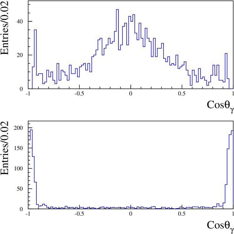
Figure 1: Angular distribution of the generated photons for $K_{S}\to 2\pi^{0}$ events after ”$K_{L}$-crash” tagging: photons reconstructed by the EMC calorimeter (top), lost photons (bottom).

3.2 Simulation of background and signal

The main expected background in this search are $K_{S}\rightarrow 2\pi^{0}$ events with two lost photons. Such losses can be due to photons 1) either out of acceptance, not reconstructed by the calorimeter or 2) merged together. For the simulation of the background Monte Carlo, MC, we use a production of $\phi\to K_{S}K_{L}$ decays corresponding to an equivalent statistics of $\sim$ 1.1 fb^-1. For the MC signal we used instead, a production equivalent to $\sim$ 18 fb^-1.

The photon properties in the simulation (resolutions and detection-efficiency) have been tuned with data using a large sample of tagged photons in $\phi\to\pi^{+}\pi^{-}\pi^{0}$ events [9] selected using only drift chamber information. The presence of additional clusters in the events due to accidental overlap with machine background, dafbkg, clusters has been taken into account by inserting these events in the MC at hit level in the simulation. The dafbkg insertion includes its rate dependence along the running period, and all other basic running conditions, such as beam parameters ($W,\overline{P}_{\phi},\overline{X}_{\phi}$) which vary run by run. The interaction of the $K_{L}$ in the calorimeter is also properly simulated.

3.3 Event preselection

After tagging, we select events by counting the number of prompt photons, $N_{\gamma}$, i.e. neutral clusters in the EMC having a time of flight consistent with a particle with $\beta=1$ coming from the interaction point. For signal counting we require $N_{\gamma}=2$, while for normalization purposes we require $N_{\gamma}=4$. A tight constraint on $\beta$ is imposed to reduce the effect of event losses due to accidental clusters from dafbkg. Moreover, to improve the rejection of the main background, $K_{S}\to 2\pi^{0}$ with two lost photons, we accept clusters with energy above 7 MeV and produced in a large angular acceptance, $|cos(\theta)|<0.93$. After this acceptance selection, the distribution of the lost photons for the background is peaked in the forward direction, as shown by the simulation in Fig. 1.

To improve the background rejection we require a veto from the QCAL calorimeter. This veto consists of rejecting events having at least one hit in QCAL with energy above the pedestal and in time with collisions. In Fig. 2, the data distribution of the difference, $\Delta T_{Q}$, between the reconstructed time of the QCAL hits, $T_{Q}$, and their expected time of flight, $TOF_{Q}$, is shown for all tagged events with $N_{\gamma}=2$. The flat distribution of hits due to machine background events shows clearly separated peaks bunched with the RF period. The sharp in-time peak observed is instead due to the lost photons from the process $K_{S}\to 2\pi^{0}$ impinging on QCAL. We veto all events in a time window, TW, defined as $|\Delta T_{Q}|<5$ ns. The QCAL veto successfully rejects $\sim 70$ % of the background while retaining a very high efficiency ($\sim 99.96$ %) on the signal.

Since we have not simulated the dafbkg events in QCAL , when applying the veto on data we should correct for the losses due to the accidental coincidence of these background hits in the time window used. A data-calibrated correction, $C_{Q}=1-P^{TW}_{Q}$, has been developed by determining $P^{TW}_{Q}$ i.e. the probability to find a spurious hit in TW. To estimate it we use two out-of-time windows one before, early, and one after, late, the collision time. The average value of the probability in these two control windows provides a first evaluation of the correction. Furthermore, to assign a systematic error to this determination, we have measured these losses also in a control sample with a ”$K_{L}$-crash” and a well reconstructed $K_{S}\to\pi^{+}\pi^{-}$ decay. This last sample does not have any photons impinging on QCAL, thus allowing us to calculate directly the losses in TW. The $\Delta T_{Q}$ distribution for these events is almost flat as shown by the overlapped distribution (points) in Fig. 2. We finally determine this probability to be: $P^{TW}_{Q}=(3.51\pm 0.04_{stat}\pm 0.26_{syst.})\%$.

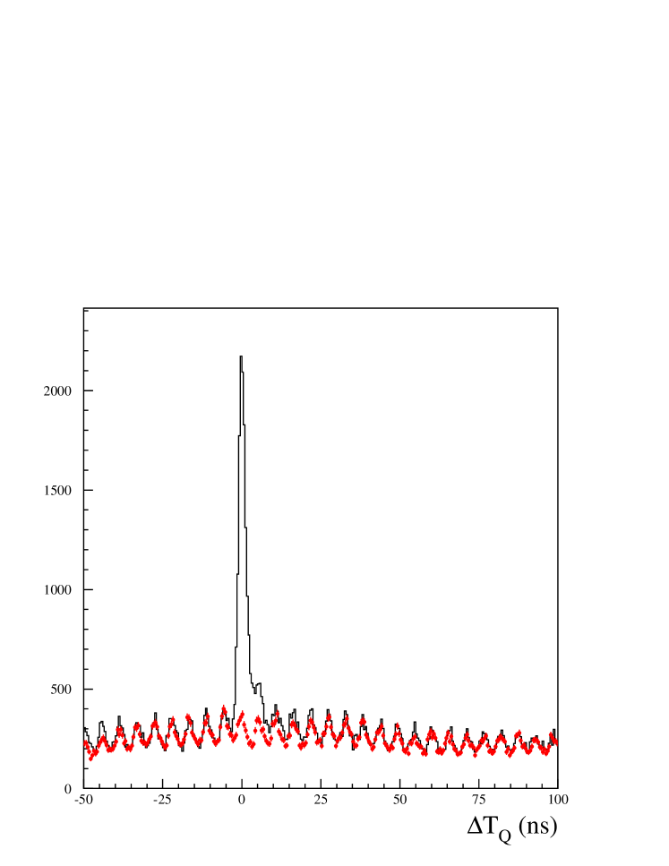
Figure 2: Inclusive distribution of the difference between the measured arrival time and the expected time of flight of prompt photons in QCAL. All hits for events tagged by a $K_{L}$-crash with $N_{\gamma}=2$ (black solid line) or with a reconstructed $K_{S}\to\pi^{+}\pi^{-}$ decay (points).

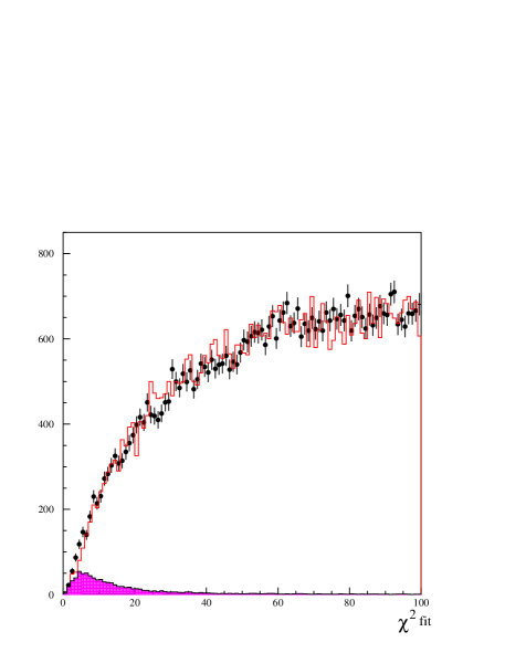
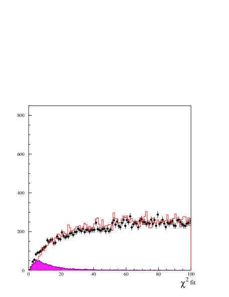
Figure 3: Distributions of $\chi^{2}_{FIT}$ for all events after tagging and $N_{\gamma}=2$ requirement: before (left) and after (right) the application of the QCAL Veto.

At the end of the acceptance and QCAL veto selection, we count 157 $\times 10^{3}$ events in data.

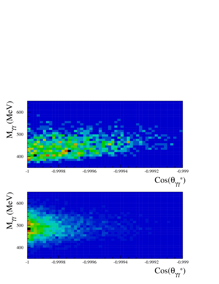
Figure 4: Scatter plot of $M_{\gamma\gamma}$ vs $cos(\theta^{*}_{\gamma\gamma})$ for simulated events: background (top) and signal (bottom).

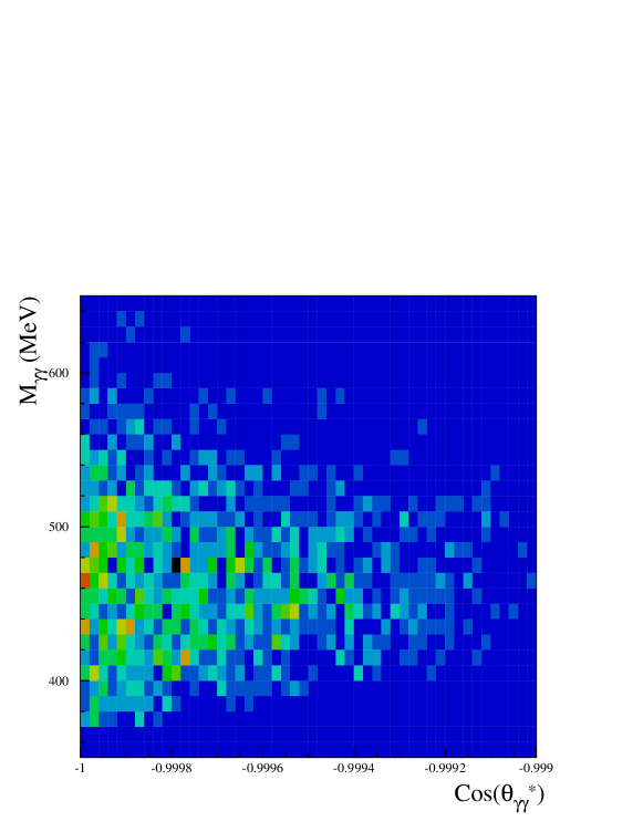
Figure 5: Scatter plot of $M_{\gamma\gamma}$ vs $cos(\theta^{*}_{\gamma\gamma})$ for data after acceptance selection, QCAL veto and $\chi^{2}_{FIT}$ cut.

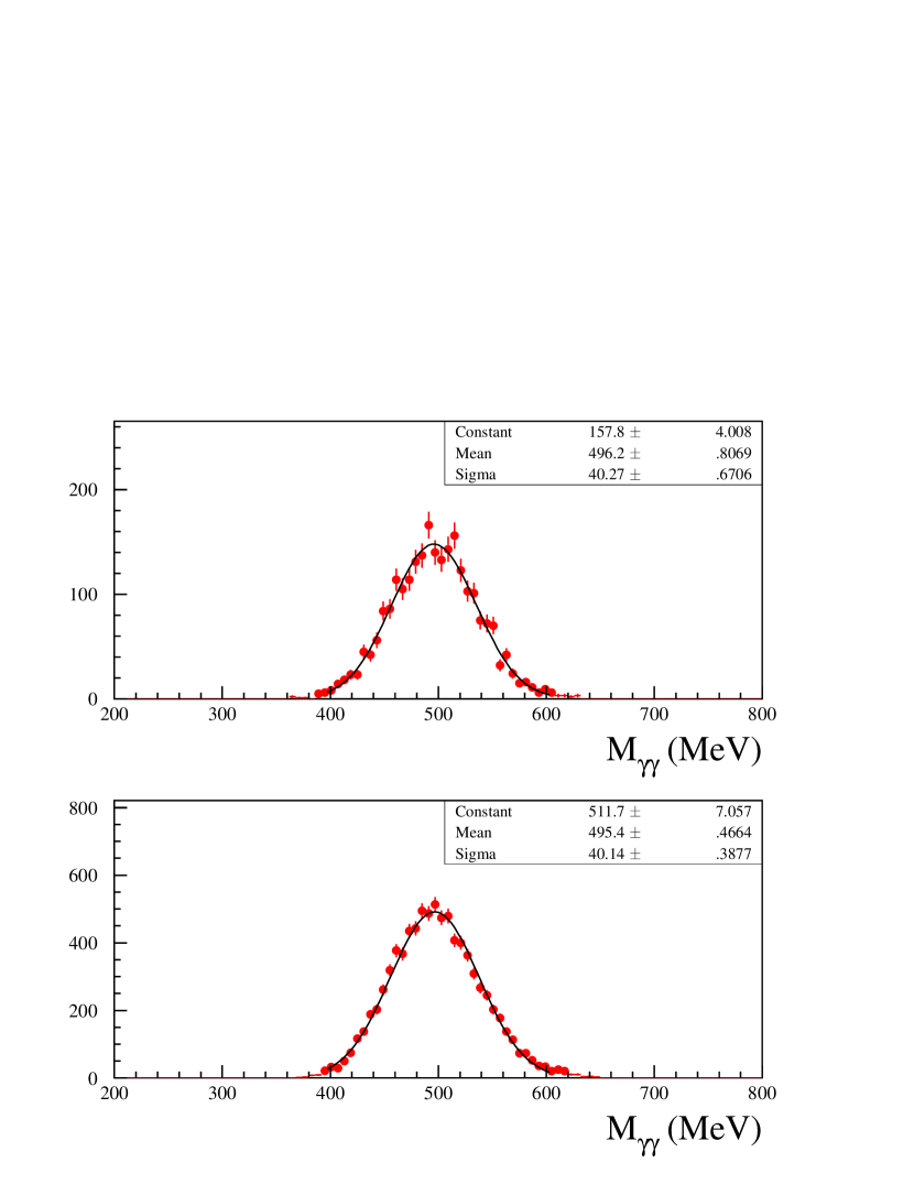
Figure 6: Distribution of the invariant mass of two photons, $M_{\gamma\gamma}$ (MeV), for the $K_{L}\to\gamma\gamma$ control sample with a neutral vertex in the fiducial region below the DC: data (top), MC samples (bottom).

3.4 Kinematic fitting and event counting

To improve the signal over background ratio (S/B), we apply a kinematic fit procedure which imposes the conservation of the $\phi$ 4-momentum at the origin, the $K_{S}$ mass and $\beta=1$ for each photon (Ndof$=$7). The fit uses the knowledge of the $K_{L}$ 4-momentum provided by the ”$K_{L}$-crash” position, W and $\overline{P_{\phi}}$. In Figs. 3.left(.right) the distribution of the $\chi^{2}$ of this procedure, $\chi^{2}_{FIT}$, is shown for data and MC after acceptance selection without (with) the application of the QCAL veto. A large amount of the background is distributed at high $\chi^{2}_{FIT}$ values while the signal is contained in the low $\chi^{2}_{FIT}$ region. In the following, we retain events by cutting at $\chi^{2}_{FIT}<20$. The Monte Carlo estimates that the signal (background) efficiency of this cut is 63.3 % (0.5%). The S/B greatly improves, from 1/500 to 1/3.

Two other variables with a high discriminating power against background are the invariant mass of the two photons, $M_{\gamma\gamma}$, and the opening angle between the two photons in the $K_{S}$ center of mass system, $\theta^{*}_{\gamma\gamma}$. Since the kinematic fit imposes the $K_{S}$  $K_{L}$ direction and the $K_{S}$ mass, we use the reconstructed variables before fit constraining. In Fig. 4.top(bottom) the 2D-plot of $M_{\gamma\gamma}$ as a function of $cos(\theta^{*}_{\gamma\gamma})$ is shown for background (signal) events. In Fig. 5, the distribution of the same scatter-plot for data is also shown.

Before fitting the data with MC shapes, we have tested our simulation ability of reproducing the signal by comparing with data a control sample of $K_{L}\to\gamma\gamma$ decaying near the beam pipe and tagged by $K_{S}\to\pi^{+}\pi^{-}$ events. Around 200 pb^-1 of data and 450 pb^-1 of Monte Carlo have been used. A kinematic fit-procedure, similar to the one of the $K_{S}\to\gamma\gamma$ sample, has been applied. The background is reduced to a negligible quantity by retaining only the events with $\chi^{2}_{FIT}({\rm KL})<20$. A gaussian fit to the $M_{\gamma\gamma}$ distribution of this control sample provides a central value of (496.2 $\pm$ 0.8) MeV in data and of (488.7 $\pm$ 0.5) MeV in Monte Carlo. This corresponds to an average energy-scale shift of $\sim$ 1% in the simulation. This motivated an in-depth data-MC comparison of energy response and resolution as a function of the incident photon energy. This study has been carried out by looking at the energy pulls of the kinematic fit with a sample of $\sim 80$ pb^-1 of $K_{S}\to 2\pi^{0}$ spread out over the entire data taking period. An ad-hoc correction has been applied to better calibrate the simulation versus the data. After applying this correction, the comparison between data and MC for the $K_{L}\to\gamma\gamma$ control sample is improved as shown by the fit to the $M_{\gamma\gamma}$ distributions shown in Fig. 6. This control sample has been also used to make a data-MC comparison for the $\chi^{2}_{FIT}({\rm KL})$ distribution. A good agreement is also observed for this variable.

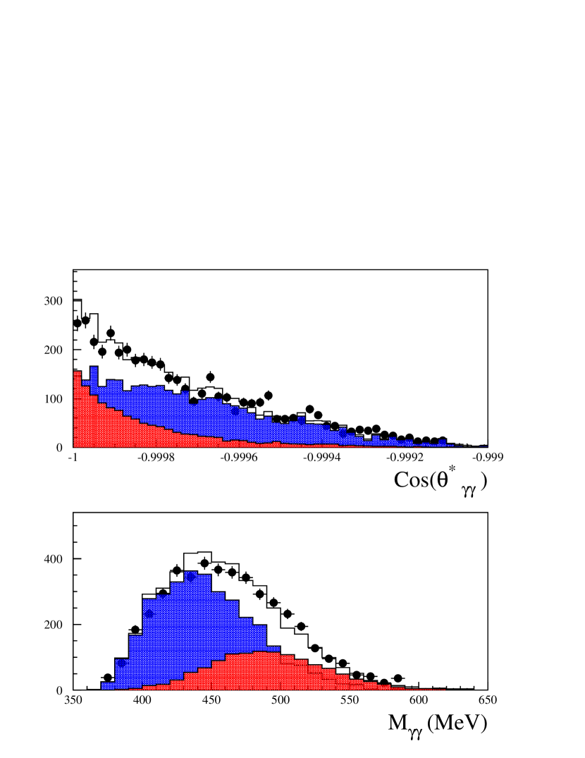
Figure 7: Distributions of data (black points) after tagging, acceptance selection and $\chi^{2}_{FIT}$ cut : cos$(\theta^{*}_{\gamma\gamma})$ (top), $M_{\gamma\gamma}$ (bottom). The superimposed colored distributions are signal and background MC shapes. Solid line is the sum of the MC shapes after fitting.

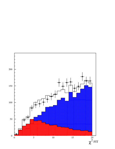
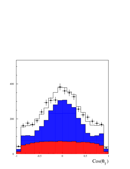
Figure 8: Distributions of data (black points) after tagging, acceptance selection and $\chi^{2}_{FIT}$ cut : $\chi^{2}_{FIT}$ (left) and inclusive cos($\theta_{\gamma}$) for the two photons in the event (right). The superimposed colored distributions are signal and background MC shapes. Solid line is the sum of MC shapes after fitting.

For the $K_{S}$-tagged events, a binned maximum-likelihood fit to the 2D $cos(\theta^{*}_{\gamma\gamma})$, $M_{\gamma\gamma}$ distribution on data is performed relying on the MC signal and background shapes. The likelihood function properly takes into account data and MC statistics of the distributions. The resulting $\chi^{2}/{\rm Ndof}$ of the fit is 1.2. The quality of the fit is shown in Fig. 7 by comparing with data the simulated shapes for mass and angular projections as weighed by the fit procedure. As expected, the $cos(\theta^{*}_{\gamma\gamma})$ distribution shows a signal shape which is much more peaked than the background to $-1$. The $M_{\gamma\gamma}$ distribution shows a well identified gaussian shape around the $K_{S}$ mass for the signal, while the background has an asymmetric shape peaked at lower mass values. We count $N(2\gamma)=600\pm 35$ signal events out of 2280 events in the 2D plot.

At the end of the analysis chain and as an independent check of the quality of the fit weights found, we show in Fig. 8.left the $\chi^{2}_{FIT}$ distribution for data and MC as weighed by the scalar factors previously determined. A similar comparison is done also for the inclusive angular photon distribution (see Fig. 8.right). The latter distribution clearly indicates the need for a flat angular dependence as expected by the uniform decay of a spin 0 particle in two photons.

4 Branching ratio evaluation and systematics

The branching ratio is evaluated with respect to the BR($K_{S}\to 2\pi^{0})$ by counting the $K_{L}$-crash tagged events with $N_{\gamma}=4$ in the same sample as follows:

$$BR(K_{S}\to 2\gamma)=\frac{N(2\gamma)}{N(2\pi^{0})}\times\frac{\varepsilon_{TOT}(2\pi^{0}|tag)}{\varepsilon_{TOT}(2\gamma|tag)}\times BR(K_{S}\to 2\pi^{0}),$$ (1)

where the total efficiencies have been evaluated by MC after $K_{S}$ tagging. We have assumed that the ratio of trigger, event classification and tagging efficiencies between the two decays is one. The signal total efficiency is the product of the efficiencies for the acceptance selection, the QCAL cut and the $\chi^{2}$ cut. Each single one has been evaluated as conditioned efficiency.

The acceptance selection efficiency for the signal, after tagging, is

$$\varepsilon_{sel}(2\gamma)=(83.2\pm 0.2_{stat}\pm 0.1_{syst})\%,$$ (2)

this large efficiency is due to the angular coverage of the calorimeter, the low energy threshold used and the flat angular distribution of the decay products. The systematic error assigned to this efficiency has been found by varying the data-MC correction curves of the cluster reconstruction efficiency. The efficiency of the QCAL cut, after tagging and acceptance, is found by MC to be $\sim$ 99.96 % . However, on data we have to apply the corrections due to accidental losses described in sec. 3.3 to obtain:

$$\varepsilon_{Q}=\varepsilon_{Q}^{MC}\times C_{Q}=(96.45\pm 0.04_{stat.}\pm 0.26_{syst.})\%.$$ (3)

The MC efficiency of the applied $\chi^{2}_{FIT}$ cut is $\varepsilon_{\chi^{2}}=(63.3\pm 0.7)\%.$ To evaluate a systematic error due to the data-MC difference in the $\chi^{2}_{FIT}$ scale, we have looked at the $K_{L}\to\gamma\gamma$ control sample by requiring loose $\chi^{2}_{FIT}$(KL) and angular cuts. A few percent contamination exists. By building $\chi^{2}_{FIT}$ cumulative distributions for data and MC and calculating their ratio at the applied cut value, a systematic error, $\Delta\varepsilon_{\chi^{2}}/\varepsilon_{\chi^{2}}$ of -0.4% is assigned to this effect.

Source	+$\Delta BR/BR$ (%)	-$\Delta BR/BR$ (%)
Signal acceptance	0.12	0.12
QCAL losses	0.02	0.26
$\chi^{2}$ scale	–	0.41
Normalization sample	0.15	0.15
QCAL TW change	0.88	0.44
$\chi^{2}$ change	0.44	0.44
2D-Fit binning	0.88	0.44
MC Energy scale	–	1.32
Total	1.33	1.61

Table 1: Contributions to the total systematic error on the BR. The first three contributions have been evaluated directly as systematics related to the signal efficiency for a given cut. The fourth contribution regards the systematics on efficiency for the normalization sample. The last four contributions have been evaluated by repeating the BR measurement while varying analysis conditions or cuts.

For the normalization we have counted $K_{S}\to 2\pi^{0}$ tagged events with $N_{\gamma}=4$. An efficiency of

$$\varepsilon_{sel}(4\gamma)=(65.0\pm 0.2_{stat}\pm{0.1}_{syst})\%$$ (4)

is found by Monte Carlo. The systematics has been evaluated, as done for the signal, by varying the data-MC correction curves of the cluster reconstruction efficiency. After correcting for $\varepsilon_{sel}(4\gamma)$, a total number of $(159.8\pm 0.5)\times 10^{6}$ $K_{S}\to 2\pi^{0}$ tagged events is obtained. Another systematic uncertainty related to accidental overlap of dafbkg clusters, shower fragmentation and merging of nearby clusters has been evaluated by repeating the measurement in an inclusive way and counting tagged events with 3, 4 and 5 photons. We get an efficiency corrected counting of $159.5\times 10^{6}$ events which agrees at $\sim 2.5$ per mil level with the number obtained with the exclusive counting.

For the BR($K_{S}\to\gamma\gamma$) we use the latest PDG [10] value of BR($K_{S}\to 2\pi^{0}$) which is $(30.69\pm 0.05)$%. The systematics connected to the counting has been evaluated by repeating the analysis in different ways. We first tested the stability of the branching ratio when modifying the width of the time window used for the QCAL veto or the applied value of the $\chi^{2}_{FIT}$ cut. In Fig. 9.left the BR changes as a function of the applied $\chi^{2}_{FIT}$ cut is shown. We then repeated the fit by applying the residual energy scale shift of +0.4% to the MC distributions and varied the bin size used in the 2D plot for fitting. In all cases, the maximum variation of the BR is used as systematic error and shown in Tab. 1. The sum in quadrature of all entries in the table is used as total systematic error. We obtain:

$$BR(K_{S}\to\gamma\gamma)=(2.27\pm 0.13(stat.)^{+0.03}_{-0.04}(syst.))\times 10^{-6}.$$ (5)

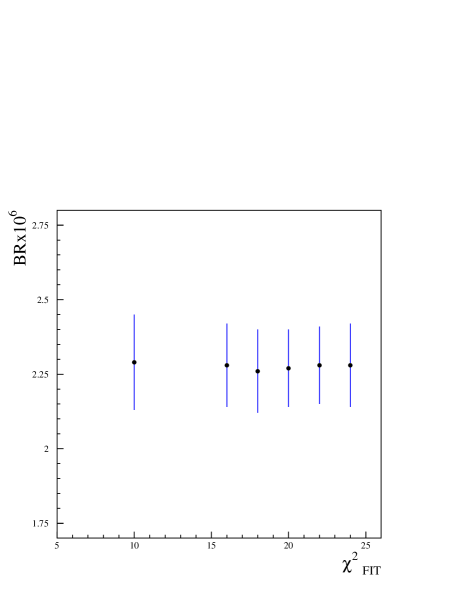
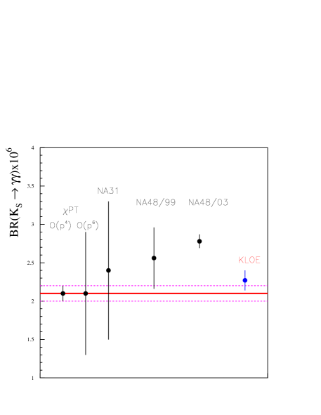
Figure 9: Variation of BR result as a function of the applied $\chi^{2}_{FIT}$ cut (left). Comparison of our measurement of BR$(K_{S}\to\gamma\gamma)$ with the other existing measurements and $O(P^{4})$ $\chi$PT predictions (right).

5 Conclusion

With a sample of 1.62 fb^-1 of $e^{+}e^{-}$ collisions at $\sqrt{s}\sim M_{\phi}$ collected with KLOE at DA$\Phi$NE, we have measured the $BR(K_{S}\to\gamma\gamma)$ with a 5.6% statistical uncertainty and a $\sim 1.5$ % systematic error. We obtain a BR result which deviates by 2.9 $\sigma$’s from the previous best precise determination, as shown in Fig. 9.right. Our measurement is also consistent, within errors, with $O(P^{4})$ $\chi PT$ predictions.

References

- [1] G. D’Ambrosio, D. Espriu, Phys. Lett. B175 (1986).
- [2] G. D. Barr, at al., Phys. Lett. B493 (1995).
- [3] J. R. Batley, at al., Phys. Lett. B551 (2003).
- [4] KLOE collaboration, M. Adinolfi et al., Nucl. Inst. Meth. A 488 (2002), 51.
- [5] KLOE collaboration, M. Adinolfi et al., Nucl. Inst. Meth. A 482 (2002), 364.
- [6] KLOE collaboration, M. Adinolfi et al., Nucl. Inst. Meth. A 483 (2002), 649.
- [7] KLOE collaboration, M. Adinolfi et al., Nucl. Inst. Meth. A 492 (2002), 134.
- [8] S. Guiducci, in: P. Lucas, S. Weber (Eds.), Proceedings of the 2001 Particle Accelerator Conference, Chicago, Il., USA, 2001.
- [9] KLOE collaboration, F. Ambrosino et al., Nucl. Inst. Meth. A 534 (2004), 403.
- [10] W.M.Yao et al., Journal of Physics G 33, (2006), 1.