Negative phase velocity in nonlinear oscillatory systems
—mechanism and parameter distributions

Abstract

Waves propagating inwardly to the wave source are called antiwaves which have negative phase velocity. In this paper the phenomenon of negative phase velocity in oscillatory systems is studied on the basis of periodically paced complex Ginzbug-Laundau equation (CGLE). We figure out a clear physical picture on the negative phase velocity of these pacing induced waves. This picture tells us that the competition between the frequency $\omega_{out}$ of the pacing induced waves with the natural frequency $\omega_{0}$ of the oscillatory medium is the key point responsible for the emergence of negative phase velocity and the corresponding antiwaves. $\omega_{out}\omega_{0}>0$ and $|\omega_{out}|<|\omega_{0}|$ are the criterions for the waves with negative phase velocity. This criterion is general for one and high dimensional CGLE and for general oscillatory models. Our understanding of antiwaves predicts that no antispirals and waves with negative phase velocity can be observed in excitable media.

I Introduction

A kind of novel waves, waves propagating inwardly to the corresponding wave sources, were predicted theoretically in sixties of the last centuryveselago , and were experimentally discovered at the beginning of this centurysmith ; vanag1 . Throughout this paper, we call this special kind of waves antiwaves (AW) for short, which have negative phase velocity, and call waves propagating forwardly from the wave source normal waves (NW). The phenomenon of negative phase velocity exists in both linearsmith and nonlinearvanag1 systems. So far, linear optical antiwaves have attracted great attention and have been introduced to applied scienceslhm ; topten1 ; aydin ; smith2 ; pendry ; topten2 ; grigorenko . While nonlinear antiwaves have been much less. Till now, scientists have found only antispirals in nonlinear systemsvanag2 ; yang ; gong ; bar ; kim . In contrast to normal spiral waves, antispiral waves propagate inwardly to the spiral tips, which serve as the sources of the waves. In some recent works, several models have been suggested to understand antispiralsvanag1 ; vanag2 . Gong and Christini have put forward an empirical criterion for the emergence of antispiralsgong . Bär et. al. have explained antispirals from the changes of the sign of $\omega$ (spiral frequency) and $k$ (spiral wave number) with the model of CGLEhagan . While these studies illuminated some aspects of antispiral waves, the mechanism and the general physical picture of antiwaves are still not completely clear. With antispiral waves in mind, some questions emerge naturally: Are there general antiwaves exist (beside antispirals) which propagate toward the wave sources? If yes, is there any common mechanism underlying these antiwaves?

This paper will deal with the above problems. The paper is organized as follows. In Section 2, we specify our nonlinear model to produce travelling nonlinear AWs by certain local periodic pacing. In Section 3, we analyze the mechanism of general nonlinear AWs, including antispirals and planar travelling antiwaves as their special cases. In Section 4, we specify the parameter regions for emergence of AWs in CGLE. The CGLE system serve as a simple example showing applications of our understanding on nonlinear AWs. Since our analysis does not depend on the detail dynamics of CGLE, we expect that the analysis in this paper is generally valid for oscillatory media. We conclude our results and give some remarks in Section 5.

II Model and nonlinear waves with negative phase velocity

Oscillatory and excitable media are two kinds of media extensively investigated in nonlinear dynamics. But antispirals are found only in oscillatory mediagong . CGLE is a typical and well known oscillatory system. Here we use 1D CGLE with local pacingzhang to explore nonlinear antiwaves.

$$\frac{\partial A}{\partial t}=A - (1+i\alpha)|A|^{2}A+(1+i\beta)\nabla^{2}A+\delta(\Omega)Fe^{-i\omega_{in}t}$$ (4)

$$\delta(\Omega)=\left\{\begin{array}[]{l@{\quad}l}1&x\in\Omega\\ 0&\mbox{otherwise}\\ \end{array}\right.$$

We conduct simulations in an aray of $N(N=256)$ sites with $\Delta x=1.0$ space discretization. Free boundary condition is used throughout the paper. Numerically, we add the periodic signal to the left boundary site of the 1D system. We fix $F=1.0$ for all simulations of this paper. The sign of the input frequency $\omega_{in}$ in Eq.(1) denotes the rotating direction of the forcing in complex plane, “+” clockwise and “-” anticlockwise. System (1) supports periodic travelling waves

$$A = \sqrt{1-k^{2}}e^{i(-\omega t+kx)}$$ (2a)

$$\omega = \alpha+(\beta-\alpha)k^{2}$$ (2b)

Equation (2b) together with the condition $0\leq k^{2}\leq 1$ define the constraint of $\omega$,

$$\alpha\leq\omega\leq\beta\mbox{ or }\beta\leq\omega\leq\alpha$$ (2c)

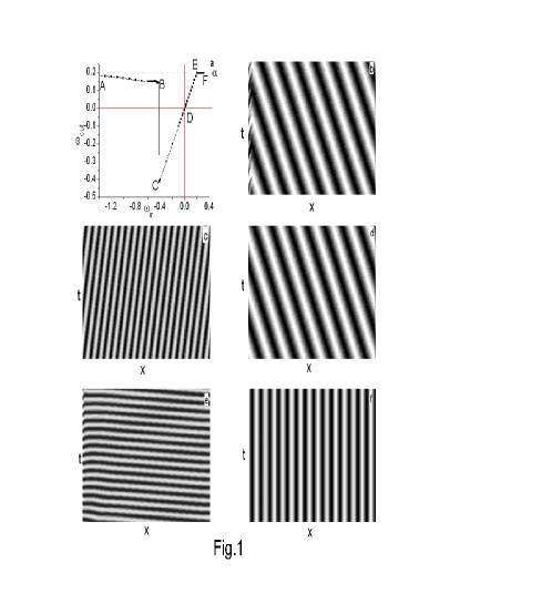
Figure 1: Numerical results of Eq.(1). $\alpha=0.2,\beta=-1.4,F=1$. (a) Input-output frequency relation. In AB and EF region, constraint Eq.(2b) forbids the complete drift $\omega_{out}=\omega=\omega_{in}$, and the system motion is governed by the local dynamics, $\omega_{out}\approx\alpha$ and $|k|\ll 1$. CE region corresponds 1:1 resonant output $\omega_{out}=\omega_{in}$. (b)-(f) Spatiotemporal patterns of the system for different parameter sets. (b) $\omega_{in}=-0.5$ (AB region), antiwaves. (c) $\omega_{in}=-0.15$ (CD region), normal waves. (d) $\omega_{in}=0.15$ (DE region), antiwaves. (e) $\omega_{in}=0.21$ (EF region). $\omega_{out}\approx\alpha=0.2$ and $k\approx 0$, practically homogeneous oscillation. (f) $\omega_{out}=\omega_{in}=0$, stationary Turning pattern.

In Fig.1(a) we plot the input-output frequency relationstamp for $\beta=-1.4,\alpha=0.2$. There are four parameter domains in Fig.1(a), corresponding to different response behaviors of the system to the local pacing. When $\omega_{in}<-0.41$, the system cannot follow the pacing frequency due to too fast pacing frequency, the output frequency of the system is thus much lower than $\omega_{in}$ and also lower than the natural frequency $(\omega_{0}=\alpha)$, $|\omega_{out}|<|\omega_{0}|$. We observe antiwaves asymptotically (see segment AB in Fig.1(a) and the evolution pattern in $t-x$ plane of Fig.1(b)). When $-0.41<\omega_{in}<0$, the system oscillates with the input frequency $\omega_{out}=\omega_{in}$ resonantly and the waves propagate normally (CD segment in Fig.1(a) and Fig.1(c)). When $0<\omega_{in}<0.2$, the system oscillates also with the input frequency $\omega_{in}$ while waves propagate inwardly to the wave source, i.e., one observes negative phase velocity (DE segment in Fig.1(a) and Fig.1(d)). When $\omega_{in}>0.2$, the system approaches asymptotically to nearly homogeneous oscillation, i.e. $k\ll 1$, $\omega_{out}\lesssim\omega_{0}=\alpha$ (antiwaves with very large phase velocity, EF segment in Fig. 1(a) and Fig.1(e)). An interesting point in Fig.1 is that we can produce both NWs and AWs with the same parameter set of $(\alpha,\beta)$ by changing the pacing frequency only. There is a special case of $\omega_{in}=0$, which locates at the boundary between NWs and AWs. We expect that this local constant force produces neither normal waves nor antiwaves. Indeed we observe in Fig.1(f) a pacing induced stationary Turning pattern.

The above numerical results demonstrate that local pacing with suitable frequency can produce AWs in nonlinear oscillatory systems indeed. These results show that nonlinear NWs and AWs are determined by the competition between the output frequency $\omega_{out}$ and the local natural frequency $\omega_{0}$ ($\omega_{0}=\alpha$ for CGLE) of oscillatory media. In summary, if $\omega_{out}$ and $\omega_{0}$ have the same sign while the absolute value of $\omega_{out}$ is smaller than that of $\omega_{0}$, we have

$$\omega_{out}\omega_{0}>0\mbox{ and}|\omega_{0}|>|\omega_{out}|\mbox{ \ \ \ Antiwaves}$$ (3a)

In other two cases we have

$$\omega_{out}\omega_{0}>0\mbox{ and }|\omega_{0}|<|\omega_{out}|$$    Normal waves (3b)

$$\omega_{out}\omega_{0}<0$$     Normal waves (3c)

It is thus the competition between $\omega_{out}$ and $\omega_{0}$ that makes the system to select the correct sign of $k$ in the dispersion relation Eq.(2b), and to determine positive ($k\omega>0$) or negative ($k\omega<0$) phase velocity (or, say, normal or anti waves).

It is emphasized that in Eq.(3) we use frequency relation between $\omega_{out}$ and $\omega_{0}$, not $\omega_{in}$ and $\omega_{0}$. Here $\omega_{out}$ is the actual frequency of the system motion. In certain cases, the oscillatory system is completely driven by the pacing and we have $\omega_{out}=\omega_{in}$. Then $\omega_{in}$ can be used instead of $\omega_{out}$ for classifying the cases of Eqs.3(a), (b) and (c) (see regions CD and DE in Fig.1(a)). In some other cases, the system cannot follow the rotation frequency of the pacing, and the asymptotic state of the system has frequency $\omega_{out}\neq\omega_{in}$, then all the above analysis describes how the competition between $\omega_{out}$ and $\omega_{0}$ produces normal and anti waves in oscillatory media. This is what happens in the segments AB and EF of Fig.1(a).

III Mechanism underlying nonlinear antiwaves

Now we try to understand the phenomena of negative phase velocity and antiwaves in CGLE. Firstly we begin with the analysis of the local dynamics of the system. Without the coupling and forcing terms the local dynamics of CGLE reads

$$\frac{dA}{dt}=A-(1+i\alpha)|A|^{2}A$$ (4)

Representing complex variable $A$ by $A=Re^{i\theta}$, we can transform Eq.(4) to

$$\left\{\begin{array}[]{l@{\quad}l}\frac{dR}{dt}=R(1-R^{3})\\ \frac{d\theta}{dt}=-\alpha R^{2}\\ \end{array}\right.$$ (7)

Eq.(5) is a typical limit cycle system with frequency $\alpha$. Every grid of system (1) is a rotator $e^{-i\alpha t}$ who rotates clockwise (anticlockwise) in complex plane if $\alpha$ is positive (negative). Therefore, Eq.(1) is an oscillatory medium, and we call $\alpha$ the local natural frequency of the system, denoted as $\omega_{0}=\alpha$.

When we force the left boundary of the system, the grids near the left boundary are driven by the pacing, and they can quickly reach their asymptotic rotation with the output frequency $\omega_{out}$. Due to the diffusion coupling, the perturbation from the left boundary can stimulate the grids distance away from the left boundary, and make these grids rotate with their natural frequency $\omega_{0}$ in the first evolution stage. In the next evolution stage, the grids away from the pacing source will be synchronized to the asymptotic frequency $\omega_{out}$, because the coupling restricts the phase difference between these grids and the grids near the left boundary. It is just the initial phase arrangement of different grids by $\omega_{out}$ and $\omega_{0}$ plays the key role in determining the sign of the phase velocity.

Figure 2: Spatial phase distribution responding the perturbation from the wave source. Frequency $\omega_{0}$ is supposed in clockwise direction. (a) $\omega_{out}\omega_{0}>0$ and $|\omega_{out}|>|\omega_{0}|$. Given a space site (with frequency $\omega_{out}$), the sites farther away from the pacing, having frequencies (near $\omega_{0}$) larger than $\omega_{out}$, rotate faster than the given site. When these sites are synchronized to the frequency $\omega_{out}$, they must have phases more advanced than the phase of the given site. This phase distribution results in negative phase velocity and AWs. (b) $\omega_{out}\omega_{0}>0$, $|\omega_{out}|>|\omega_{0}|$ and (c) $\omega_{out}\omega_{0}<0$. By the same argument as (a), the sites farther away from the pacing source have phase delay with respect to the given site. We can observe positive phase velocity and NWs.

Now we analyze the three types of Eq.(3). First, we suppose that the pacing generated frequency $\omega_{out}$ is in the same direction with the local natural frequency $\omega_{0}$ and we have $|\omega_{0}|>|\omega_{out}|$ (case Eq. (3a)). The grids near the left boundary rotate initially slower than its neighbor grids farther away from the pacing source. When synchronization of all these grids are reached the phase of the latter must be more in advance than that of the former. One thus observes phase propagation towards to the pacing source, an interesting phenomenon of negative phase velocity. This kind of phase setting is shown in Fig.2(a).

Second, if $\omega_{out}$ and $\omega_{0}$ have the same sign while $|\omega|>|\omega_{0}|$ (case Eq.(3b)), the initial phase distribution of the grids is such prepared for the asymptotical travelling waves that any grid in the 1D chain must have some phase delay in comparison with its neighbor grids nearer the pacing source as shown in Fig.2(b). In this case one can observe normal forward propagating waves. Third, if the two frequencies $\omega_{out}$ and $\omega_{0}$ have opposite rotation directions ($\omega_{0}\omega_{out}<0$, case Eq.(3c)), one can observes phase distribution of grids of Fig.2(c) yielding normal forward waves.

Now we can give some clear conclusions on the problem of antiwaves and negative phase velocity. These conclusions are valid not only for CGLE systems, but also for general oscillatory systems. We suppose that a system is oscillatory with local dynamics having bulk frequency $\omega_{0}$ vanag1 ; gong and the medium supports periodic waves with frequency $\omega_{out}$ generated by an arbitrary perturbation source. If $\omega_{out}$ and $\omega_{0}$ have the same sign and $|\omega_{out}|<|\omega_{0}|$, we can surely produce antiwaves, and we can produce normal waves in all other cases, except two no generic critical cases: $k=0$ (producing homogeneous oscillations) and $\omega_{out}=0$ (producing stationary Turning patterns). It is emphasized that our analysis based on the pictures of Fig.2 does not use any special dynamic structure of CGLE, and thus does not need the requirement that the system is near Hopf bifurcation condition. This generality has never been explored in previous analysis on the problems of negative phase velocity. In our analysis, local oscillation (i.e., nonzero $\omega_{0}$) is a necessary condition for negative phase velocity. If the local dynamics of a medium does not have oscillation, we have $\omega_{0}=0$. It is clear from Eq.(3) that the system with $\omega_{0}=0$ can support only normally propagating waves. All excitable media have local frequency $\omega_{0}=0$, and we can therefore answer a previously raised question about antispirals in excitable mediagong : antiwaves (including antispirals) can never be found in excitable media. We have numerically computed CGLE for many other parameter sets, and computed different chemical reaction diffusion models with oscillatory and excitable local dynamics, the above conclusions have been fully confirmed.

IV Parameter domain for antiwaves in CGLE system

The analysis of Eq.(3) and the physical mechanism of Fig.2 are valid for general oscillatory systems. CGLE is a kind of oscillatory system universally appearing around Hopf bifurcation from a homogeneous stationary states to homogeneous oscillation. It is thus interesting to classify parameter domains for normal and anti waves of CGLE. In this section we focus on specifying the domain of antiwaves of CGLE in $(\alpha,\beta,\omega_{out})$ parameter space.

The motion of periodically forced CGLE can be periodic, quasiperiodic and chaotic. Here we are interested only in periodic travelling wave states. Far away from the pacing boundary, travelling waves must have solution of Eq.(2a) and the frequency $\omega_{out}$ must obey condition Eq.(2c). This condition is required for all periodic travelling waves, including both NW and AW. On the other hand, the conditions of Eq.(3) can be used to classify NW and AW. Eqs.(2c) and (3) together completely determine the parameter domains of NW and AW of CGLE.

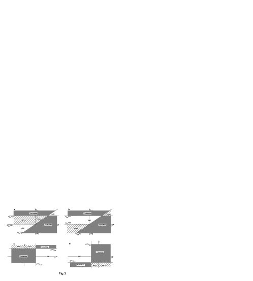
Figure 3: Schematic figures of phase diagrams of CGLE, which are drawn, based on Eq.(2c) and (3). (a) Phase diagram in $\omega_{out}-\alpha$ plane with $\beta>0$ fixed. In the grey regions marked “Forbidden”, travelling waves cannot be realized due to the condition of Eq.(2c). The blank region marked AW is antiwave region, characterized by Eq.(3a). The shadowed region marked NW1 (NW2) is a part of normal wave region, characterized by Eq.(3b) (by Eq.(3c)). (b) The same as (a) with $\alpha>0$ fixed and the distribution of various characteristic domains is plotted in $\beta-\omega_{out}$ plane. (c) The same as (a) with $\omega_{out}>0$ fixed and the domain distribution is plotted in $\alpha-\beta$ plane. (d) The same as (c) with $\omega_{out}<0$. (d) and (c) are symmetric against the symmetry center $(\alpha,\beta)=(0,0)$.

In Fig.3(a) we present domain distribution of NWs and AWs in $\alpha-\omega_{out}$ plane with $\beta$ fixed. In the parameter region marked “Forbidden”, the parameters do not satisfy the constraint of Eq.(2c), and no periodic travelling wave exists in this domain. In the blank region (the blow-left and up-right parts), the parameters satisfy Eq.(2c) and the conditions of Eq.(3a), we can observe AWs. In the shadowed region marked NW1 (NW2), the parameters satisfy Eq.(2c) and Eq.(3b) (and Eq.(3c)), and NWs are produced. In Figs.3(b) and 3(c) we do exactly the same as Fig.3(a) with $\alpha$ and $\omega$ fixed, respectively. Figs. 3(a), 3(b) and 3(c) are obtained for arbitrary positive $\beta$, $\alpha$ and $\omega_{out}$. For negative $\beta$, $\alpha$ and $\omega_{out}$ we can directly obtain domain distribution diagrams from Fig.3(a), 3(b) and 3(c), replacing $\alpha$, $\omega_{out}$; $\beta$, $\omega_{out}$; and $\alpha$, $\beta$ by $-\alpha$, $-\omega_{out}$; $-\beta$, $-\omega_{out}$; and $-\alpha$, $-\beta$, respectively (e.g., see Fig.3(d)).

V Conclusion

In conclusion, we have found interesting phenomenon of negative phase velocity (antiwaves) induced by local pacing, and revealed the common mechanism underlying antiwaves: the competition between the actual system frequency $\omega_{out}$ and the local natural frequency $\omega_{0}$ selects the correct sign of the wave number $k$ in the dispersion relation Eq.(2b) to produce either normal waves or antiwaves. If condition $\omega\omega_{0}>0$ and $|\omega|<|\omega_{0}|$ are satisfied, antiwaves can emerge definitely. To our best knowledge, it is the first time to emphasize that both signs and values of $\omega$ and $\omega_{0}$ play essential roles in producing antiwaves. This understanding gives a convincing answer to the problem why no antispirals and antiwaves have been observed in excitable media. The criterion of antiwaves (Eq.(3a) and Fig.2(a)) is expected to be valid for general oscillatory systems, and this goes again beyond the previous results of negative phase velocity of CGLE.

References

- (1) V. G. Veselago, Sov. Phys. Usp. 10, 509 (1968).
- (2) R. A. Shelby, D. R. Smith, and S. Schultz, Science 292, 77 (2001).
- (3) V. K. Vanag and I. R. Epstein, Science 294, 835 (2001).
- (4) C. G. Parazzoli, D. B. Brock, and S. Schultz, Phys. Rev. Lett. 90, 107401 (2003).
- (5) The News and Editorial Staffs, The Runners-Up, Science 302, 2043 (2003).
- (6) K. Aydin, I. Bulu, and E. Ozbay, Opt. Express 13, 8753 (2005).
- (7) D. R. Smith, J. B. Pendry, M. C. K. Wiltshire, Science 305, 788 (2004).
- (8) J. B. Pendry, Science 306, 1353 (2004).
- (9) P. V. Parimi, W. T. Lu, P. Vodo and S. Sridhar, Nature 426, 404 (2003).
- (10) A. N. Grigorenko, A. K. Geim, H. F. Gleeson, Y. Zhang, A. A. Firsov, I. Y. Khrushchev and J. Petrovic, Nature 438, 17 (2005).
- (11) V. K. Vanag and I. R. Epstein, Phys. Rev. Lett. 87, 228301 (2001); Phys. Rev. Lett. 88, 088303 (2002).
- (12) L. Yang, M. Dolnik, A. M. Zhabotinsky, and I. R. Epstein, J. Chem. Phys. 117, 7259 (2002).
- (13) Y. Gong and D. J. Christin, Phys. Rev. Lett. 90, 088302 (2003); Phys. Lett. A 331, 209 (2004).
- (14) L. Brusch, E. M. Nicola, and M. Bär, Phys. Rev. Lett. 92, 089801 (2004); E. M. Nicola, L. Brusch, and M. Bär, J. Phys. Chem. B 108 14733 (2004).
- (15) P. Kim, T. Ko, H. Jeong, and H. Moon, Phys. Rev. E 70, R065201 (2004).
- (16) P. S. Hagan, SIAM J. Appl. Math. 42, 762 (1982).
- (17) H. Zhang, B. Hu, G. Hu, Q. Ouyang, and J. Kurths, Phys. Rev. E 66 046303 (2002); H. Zhang, Z. Cao, N. Wu, H. Ying and G. Hu, Phys. Rev. Lett. 94, 188301 (2005).
- (18) I. S. Aranson, and L. Kramer, Rev. Mod. Phys 74, 99 (2002).
- (19) A. T. Stamp, and G. V. Osipov, Chaos 12, 931 (2002).