Spectropolarimetric signatures
of Earth–like extrasolar planets

Abstract

We present results of numerical simulations of the flux (irradiance), $F$, and the degree of polarization (i.e. the ratio of polarized to total flux), $P$, of light that is reflected by Earth–like extrasolar planets orbiting solar–type stars, as functions of the wavelength (from 0.3 to 1.0 $\mu$m, with 0.001 $\mu$m spectral resolution) and as functions of the planetary phase angle. We use different surface coverages for our model planets, including vegetation and a Fresnel reflecting ocean, and clear and cloudy atmospheres. Our adding-doubling radiative transfer algorithm, which fully includes multiple scattering and polarization, handles horizontally homogeneous planets only; we simulate fluxes and polarization of horizontally inhomogeneous planets by weighting results for homogeneous planets. Like the flux, $F$, the degree of polarization, $P$, of the reflected starlight is shown to depend strongly on the phase angle, on the composition and structure of the planetary atmosphere, on the reflective properties of the underlying surface, and on the wavelength, in particular in wavelength regions with gaseous absorption bands. The sensitivity of $P$ to a planet’s physical properties appears to be different than that of $F$. Combining flux with polarization observations thus makes for a strong tool for characterizing extrasolar planets. The calculated total and polarized fluxes will be made available through the CDS.

keywords: techniques: polarimetric – stars: planetary systems – polarization

1 Introduction

Polarimetry has been recognized as a powerful technique for enhancing the contrast between a star and an exoplanet, and hence for the direct detection of exoplanets, because, integrated over the stellar disk, the direct light of a solar type star can be considered to be unpolarized (see Kemp et al. 1987), while the starlight that has been reflected by a planet will generally be polarized because it has been scattered within the planetary atmosphere and/or reflected by the surface (if there is any). The degree of polarization of the reflected starlight (i.e. the ratio of the polarized to the total flux) is expected to be especially large around a planet’s quadrature (i.e. when the planet is seen at a phase angle of 90^∘), where the angular separation between a star and its exoplanet is largest, and which is thus an excellent phase angle for the direct detection of light from an exoplanet.

Besides from detecting exoplanets, polarimetry can also be used to characterize exoplanets, because the planet’s degree of polarization as a function of wavelength and/or planetary phase angle is sensitive to the structure and composition of the planetary atmosphere and underlying surface. This application of polarimetry is well-known from remote-sensing of solar system planets, in particular Venus (see Hansen & Hovenier 1974a, b, for a classic example), but also the outer planets (see Shkuratov et al. (2005) for recent, Hubble Space Telescope polarization observations of Mars, and Joos et al. (2005) and Schmid et al. (2006) for Earth-based polarimetry of Uranus and Neptune). Note that Venus is much more favourable to observe with Earth-based polarimetry than the outer solar system planets, because as an inner planet, Venus can be observed from small to large phase angles (including quadrature), whereas the outer planets are always seen at small phase angles, where the observed light is mostly backscattered light and degrees of polarization are thus usually small (see Stam et al. (2004) for examples of the phase angle dependence of the degree of polarization of starlight reflected by gaseous exoplanets).

The strengths of polarimetry for exoplanet detection and characterization have been recognized and described before, for example by Seager et al. (2000); Saar & Seager (2003); Hough & Lucas (2003); Stam (2003); Stam et al. (2003, 2004, 2005), who presented numerically calculated fluxes and degrees of polarization of gaseous exoplanets. Note that Seager et al. (2000); Saar & Seager (2003), and Hough & Lucas (2003) concentrate on polarization signals of exoplanets that are spatially unresolvable from their star, in other words, the polarized flux of the planet is added to a huge background of unpolarized stellar flux, while Stam (2003) and Stam et al. (2003, 2004, 2005) aim at spatially resolvable planets, which are observed with a significantly smaller unpolarized, stellar background signal. Polarization signals of spatially unresolved non-spherical planets were presented by Sengupta & Maiti (2006). Note that their calculations include only single scattered light, and not all orders of scattering (like those of Seager et al. (2000) and Stam et al. (2004)), which, except for planetary atmospheres with a very thin scattering or a very thick absorption optical thickness, significantly influences the predicted degree of polarization, because multiple scattered light usually has a (much) lower degree of polarization than singly scattered light.

Examples of ground-based telescope instruments that use polarimetry for exoplanet research are PlanetPol, which aims at detecting spatially unresolved gaseous exoplanets (see Hough et al. 2006a, b, and references therein) and SPHERE (Spectro-Polarimetric High-contrast Exoplanet Research) (see Beuzit et al. 2006, and references therein) which aims at detecting spatially resolved gaseous exoplanets. SPHERE is being designed and build for ESO’s Very Large Telescope (first light is expected in 2010) and has a polarimeter based on the ZIMPOL (Zürich Imaging Polarimeter) technique (see Schmid et al. 2005; Gisler et al. 2004, and references therein). Polarimetry is also a technique used in SEE-COAST (the Super Earths Explorer – Coronographic Off-Axis Telescope), a space-based telescope for the detection and the characterization of gaseous exoplanets and large rocky exoplanets, so called ’Super-Earths’, (Schneider et al. 2006), that has been proposed to ESA in response to its 2007 Cosmic Vision call.

The design and development of instruments for the direct detection of (polarized) light of exoplanets requires sample signals, i.e. total and polarized fluxes as functions of the wavelength and as functions of the planetary phase angle. Previously (see e.g. Stam et al. 2004), we presented numerically calculated flux and polarization spectra of light reflected by giant, gaseous exoplanets, integrated over the illuminated and visible part of the planetary disk, for various phase angles. In this paper, we present similar spectra but now for light reflected by Earth–like exoplanets. Our radiative transfer calculations fully include single and multiple scattering and polarization. The model atmospheres contain either only gaseous molecules or a combination of gas and clouds. The clouds are modeled as horizontally homogeneous layers of scattering (liquid water) particles, which allows surface features to show up in the reflected light even if the planet is fully covered. We show results for surfaces with wavelength independent albedos ranging from 0.0 to 1.0, as well as for surface albedos representative for vegetation, and ocean. The ocean surface includes Fresnel reflection.

Our disk integration method is based on the expansion of the radiation field of the planet into generalized spherical functions (Stam et al. 2006), and pertains to horizontally homogeneous planets only (the planetary atmospheres can be vertically inhomogeneous). The main advantage of this method, compared to more conventional integration of calculated fluxes and polarization over a planetary disk is that the flux and polarization of a planet can be rapidly obtained for an arbitrary number of planetary phase angles, without the need of new radiative transfer calculations for every new phase angle. This is indeed an important advantage, because polarization calculations are generally very computing time consuming compared to mere flux calculations. The disadvantage of our method is obviously its inability to handle horizontally inhomogeneous planets. In this paper, we will approximate the light reflected by horizontally inhomogeneous planets by using weighted sums of light reflected by horizontally homogeneous planets. With such quasi horizontally inhomogeneous planets, we can still get a good impression of the influence of horizontal inhomogeneities on the reflected signals. When in the future direct observations of Earth-like exoplanets become available, the more conventional disk integration method can straightforwardly be applied.

Our numerical simulations cover the wavelength region from 0.3 to 1.0 $\mu$m, thus from the UV to the near-infrared. The spectral resolution of our simulations is 0.001 $\mu$m, which is high enough for spectral features due to absorption of atmospheric gases to be clearly visible in the flux and polarization spectra. Such high spectral resolution observations of Earth-like exoplanets will not be possible for years to come; our spectra, however, show the potential information content of high spectral resolution spectra, and they can be convolved with instrument response functions to simulate observations by instruments with a lower spectral resolution. To allow the use of our flux and polarization spectra for such applications, they will be made available at the CDS.

Flux spectra of light reflected by Earth-like exoplanets have been presented before (e.g. by Tinetti et al. 2006b, a, c; Montañés-Rodríguez et al. 2006; Turnbull et al. 2006). New in this paper are flux spectra with the corresponding polarization spectra. Numerically calculated degrees and directions of polarization of exoplanets are not only useful for the design and building of polarimeters for exoplanet research, as described above, but also for the design, building, and use of instruments that aim at measuring only fluxes of exoplanets. Namely, unless carefully corrected for, the optical components of such instruments will be sensitive to the state of polarization of the observed light. Consequently, the measured fluxes will depend on the state of polarization of the observed light. Provided an instrument’s polarization sensitivity is known, our simulations can help to estimate the error that arises in the measured fluxes. Note that in order to actually correct measured fluxes for instrumental polarization sensitivity, knowing the polarization sensitivity of an instrument does not suffice; the state of polarization of the incoming light should be measured along with the flux (see e.g. Stam et al. 2000b, for a discussion on flux errors in remote-sensing due to instrumental polarization sensitivity).

Stam & Hovenier (2005) discuss another reason to include polarization into numerical simulations of light reflected by exoplanets: neglecting polarization induces errors in numerically calculated fluxes (thus also in e.g. the planet’s albedo). The reason for these errors is that light can only be fully described by a 4-vector (see Sect. 2.1), and a scattering process is only fully described by a $4\times 4$ matrix. Consequently, the flux resulting from the scattering of unpolarized light differs usually from the flux resulting from the scattering of polarized light. Because the unpolarized starlight that is incident on a planet is usually polarized upon its first scattering, second and higher orders of scattering induce errors in the fluxes when polarization is neglected (see also Lacis et al. 1998; Mishchenko et al. 1994). For gaseous exoplanets, with their optically thick atmospheres, the flux errors due to neglecting polarization can reach almost 10 $\%$ (Stam & Hovenier 2005). For Earth-like exoplanets, with optically thinner atmospheres, we show in this paper that the errors are smaller: typically a few percent at short wavelengths ( 0.4 $\mu$m) and they decrease with wavelength (see Sect. 5).

This paper has the following structure. In Sect. 2, we describe how we define and calculate flux vectors and polarization for extrasolar planets. In Sect. 3, we describe the atmospheres and surfaces of our Earth–like model extrasolar planets. In Sect.4, we present the numerically calculated fluxes and degrees of polarization of starlight that is reflected by our Earth-like model planets for both horizontally homogeneous planets and the so–called quasi horizontally inhomogeneous planets, i.e. weighted mixtures of light reflected by horizontally homogeneous planets. Section 5, finally, contains the summary and discussion of our results.

2 Describing and calculating reflected starlight

2.1 Flux vectors and polarization

The flux (irradiance) and state of polarization of stellar light that is reflected by a planet can fully be described by a flux (column) vector ${\bf F}$ as follows

$${\bf F}=\left[F,Q,U,V\right].$$ (1)

Here, $F$ is the total reflected flux divided, $Q$ and $U$ describe the linearly polarized flux, and $V$ the circularly polarized flux (see e.g. Hansen & Travis 1974; Hovenier et al. 2004). The fluxes $F$, $Q$, $U$, and $V$ in Eq. 1 have the dimension W m^-2 m^-1.

Fluxes $Q$ and $U$ are defined with respect to a reference plane, for which we, unless stated otherwise, chose the so-called planetary scattering plane, i.e. the plane through the centers of the star and the planet, that also contains the observer. We define $F_{\rm x^{\circ}}$ as the flux that is measured through a polarization filter oriented perpendicular to the direction of propagation of the light, and with its optical axis making an angle of $x^{\circ}$ with the reference plane. The angle is measured rotating from the reference plane to the filter’s optical axis in the anti–clockwise direction when looking in the direction of propagation of the light (see Hansen & Travis 1974; Hovenier et al. 2004). The so–called (linearly) polarized fluxes, $Q$ and $U$, can then in principle be obtained with the following flux measurements

$$Q = F_{0^{\circ}}-F_{90^{\circ}},$$ (2)

$$U = F_{45^{\circ}}-F_{135^{\circ}}.$$ (3)

Expressed in the fluxes of Eqs. 2 and 3, the total flux, $F$, is simply equal to either $F_{0^{\circ}}+F_{90^{\circ}}$ or $F_{45^{\circ}}+F_{135^{\circ}}$. Note that modern polarimetry has much more options available than polarization filters, such as various types of modulators (see e.g. Gandorfer et al. 2004; Gisler et al. 2004; Schmid et al. 2005; Keller 2006).

Flux vectors can be transformed from one reference plane to another, e.g. from the planetary scattering plane (which depends on the location of the planet on the sky with respect to its star) to the optical plane of a polarimeter, by multiplying them with a so–called rotation matrix ${\bf L}$ that is given by (see Hovenier et al. 2004)

$${\bf L}(\beta)=\left[\begin{array}[]{cccc}1&0&0&0\\ 0&\cos{2\beta}&\sin{2\beta}&0\\ 0&-\sin{2\beta}&\cos{2\beta}&0\\ 0&0&0&1\end{array}\right].$$ (4)

Angle $\beta$ is the angle between the two reference planes, measured rotating in the anti–clockwise direction from the old to the new plane when looking in the direction of propagation of the light ($\beta~{}\geq~{}0$).

The direction of linear polarization with respect to the reference plane is given by angle $\chi$, which can be found using

$$\tan 2\chi=U/Q,$$ (5)

where the convention is to choose $\chi$ such that $0\leq\chi<\pi$, and such that $\cos 2\chi$ and $Q$ have the same sign (see Hansen & Travis 1974; Hovenier et al. 2004). In particular, when $\chi=90^{\circ}$ ($\chi=0^{\circ}$), $Q<0$ ($Q>0$), and the direction of polarization is perpendicular (parallel) to the reference plane, i.e. perpendicular (parallel) to the imaginary line connecting the centers of the star and the planet as seen from the observer.

The degree of polarization of the reflected starlight is defined as

$$P=\frac{\sqrt{Q^{2}+U^{2}+V^{2}}}{F}.$$ (6)

Note that $P$ as defined in Eq. 6 is independent of the choice of reference plane. Assuming that the planet is mirror–symmetric with respect to the planetary scattering plane, and assuming the incoming starlight is unpolarized, the disk–integrated Stokes parameters $U$ and $V$ will equal zero because of symmetry (the incoming starlight is unpolarized). In that case, we can use an alternative definition of the degree of polarization (see also Eq. 2), namely

$$P_{\rm s}=-\frac{Q}{F}=-\frac{F_{0^{\circ}}-F_{90^{\circ}}}{F_{0^{\circ}}+F_{90^{\circ}}}.$$ (7)

For $P_{\rm s}>0$, the light is polarized perpendicular to the reference plane (i.e. $\chi=90^{\circ}$), and for $P_{\rm s}>0$, the light is polarized parallel to the reference plane (i.e. $\chi=0^{\circ}$). The subscript $s$ (from ”sign”) in $P_{\rm s}$ thus indicates that the direction of polarization is included in the definition of the degree of polarization.

2.2 Computing reflected starlight

Given a spatially unresolved spherical planet with radius $r$, the flux vector ${\bf F}$ (see Eq. 1) of stellar light with wavelength $\lambda$ that has been reflected by the planet and that arrives at an observer at a distance $d$ (with $d\gg r$) can be written as (see also Stam et al. 2006)

$${\bf F}(\lambda,\alpha)=\frac{r^{2}}{d^{2}}\hskip 2.27626pt\frac{1}{4}{\bf S}(\lambda,\alpha)\hskip 2.27626pt\pi{\bf F}_{0}(\lambda).$$ (8)

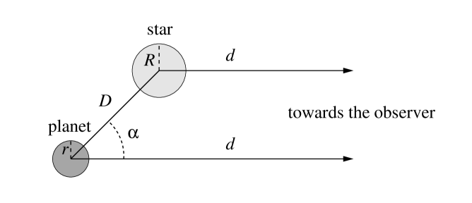
Figure 1: Top-view sketch of the geometries involved in observing extrasolar planets: $D$ is the distance between the star and the planet, $R$ is the radius of the star, $d$ is the distance between the planetary system and the observer, $r$ is the radius of the planet, and $\alpha$ is the planetary phase angle. We assume that $D\gg R$ and that $d\gg r$.

Here, $\alpha$ is the planetary phase angle, i.e. the angle between the star and the observer as seen from the center of the planet. Note that $\alpha=180^{\circ}-\Theta$, with $\Theta$ the total scattering angle of the incoming starlight. A sketch of the geometries is given in Fig. 1.

Furthermore in Eq. 8, ${\bf S}$ is the $4\times 4$ planetary scattering matrix (see below and Stam et al. 2006), and ${\bf F}_{0}$ represents the flux (column) vector describing the stellar light that is incident on the planet, with $\pi F_{0}$ the stellar flux that arrives at the planet (in W m^-2 m^-1) measured perpendicular to the direction of propagation of the stellar light. Integrated over the stellar disk, the stellar light of a solar–type star can be assumed to be unpolarized (Kemp et al. 1987), hence in the following we will use ${\bf F}_{0}(\lambda)=F_{0}(\lambda)[1,0,0,0]=F_{0}(\lambda){\bf 1}$, with ${\bf 1}$ the unit column vector. We assume that the starlight is unidirectional when it arrives at the planet.

The planetary scattering matrix, ${\bf S}$, depends on the planetary phase angle, $\alpha$, and on the wavelength, $\lambda$. The relation between ${\bf S}$ and $\alpha$ and $\lambda$ depends on the composition and structure of the planetary atmosphere and on the planetary surface. This dependence will be further described in Sect. 3. Using the planetary scattering plane as the reference plane, and assuming the planet is mirror–symmetric with respect to this reference plane, matrix ${\bf S}$ is given by (see Stam et al. 2006, 2004)

$${\bf S}(\lambda,\alpha)=\left[\begin{array}[]{cccc}a_{1}(\lambda,\alpha)&b_{1}(\lambda,\alpha)&0&0\\ b_{1}(\lambda,\alpha)&a_{2}(\lambda,\alpha)&0&0\\ 0&0&a_{3}(\lambda,\alpha)&b_{2}(\lambda,\alpha)\\ 0&0&-b_{2}(\lambda,\alpha)&a_{4}(\lambda,\alpha)\end{array}\right].$$ (9)

Matrix element $a_{1}$ is usually called the planetary phase function. Matrix ${\bf S}$ is normalized such that the average of $a_{1}$ over all directions equals the planet’s (monochromatic) Bond albedo, $A_{\rm B}$, which is the fraction of the incident stellar flux that is reflected by the planet in all directions, i.e.

$$\frac{1}{4\pi}\int_{4\pi}a_{1}(\lambda,\alpha)\hskip 2.27626ptd\omega=\frac{1}{2}\int_{0}^{\pi}a_{1}(\lambda,\alpha)\hskip 2.27626pt\sin\alpha\hskip 2.27626ptd\alpha\equiv A_{\rm B}(\lambda),$$ (10)

where $d\omega$ is an element of solid angle. The (monochromatic) geometric albedo, $A_{\rm G}$, of a planet is the ratio of the flux reflected by the planet at $\alpha=0^{\circ}$, to the flux reflected by a Lambertian surface subtending the same solid angle (i.e. $\pi r^{2}/d^{2}$) on the sky. Thus,

$$A_{\rm G}(\lambda)=\frac{F(\lambda,0^{\circ})}{F_{0}(\lambda)}\hskip 2.27626pt\hskip 2.27626pt\frac{d^{2}}{\pi r^{2}}=\frac{1}{4}~{}a_{1}(\lambda,0^{\circ}).$$ (11)

From Eqs. 8 and 9 it is clear that with unpolarized incident stellar light, the observable total flux, $F$, of starlight that is reflected by a planet is given by

$$F(\lambda,\alpha)=\frac{r^{2}}{d^{2}}\hskip 2.27626pt\frac{1}{4}a_{1}(\lambda,\alpha)\hskip 2.27626pt\pi F_{0}(\lambda),$$ (12)

and the observable polarized flux, $Q$, by

$$Q(\lambda,\alpha)=\frac{r^{2}}{d^{2}}\hskip 2.27626pt\frac{1}{4}b_{1}(\lambda,\alpha)\hskip 2.27626pt\pi F_{0}(\lambda).$$ (13)

With unpolarized incident stellar light and a planet that is mirror-symmetric with respect to the planetary scattering plane, it follows from Eqs. 12 and 13 that the degree of polarization $P_{\rm s}$ of the starlight that is reflected by the planet can simply be rewritten as (cf. Eq. 7)

$$P_{\rm s}(\lambda,\alpha)=-\frac{b_{1}(\lambda,\alpha)}{a_{1}(\lambda,\alpha)}.$$ (14)

The degree of polarization of the reflected light then thus solely depends on the planetary scattering matrix elements $a_{1}$ and $b_{1}$. Because both $P$ (Eq. 6) and $P_{\rm s}$ (Eqs. 7 and 14) are relative measures, they are independent of the radii $r$ and $R$, the distances $D$ and $d$, which is very convenient when analyzing direct observations of extrasolar planets at unknown distances.

To calculate the flux and degree of polarization of light reflected by a given Earth-like model planet (see Sect. 3) across a given wavelength region and for a given planetary phase angle, we have to calculate elements of the planetary scattering matrix ${\bf S}$ (Eq. 9). For this we use the algorithm as described in Stam et al. (2006), which combines an accurate adding-doubling algorithm (van de Hulst 1980; de Haan et al. 1987) to compute the radiative transfer through a locally plane-parallel planetary model atmosphere, and a fast, numerical, disk-integration algorithm, to integrate the reflected flux vectors across the illuminated and visible part of the planetary disk.

Our disk-integration algorithm (Stam et al. 2006) is very efficient, and its computing time depends only little on the number of planetary phase angles for which the disk-integrated flux vectors are calculated. The disadvantage of the current version of the algorithm is that it can only handle horizontally homogeneous planets (which are mirror-symmetric with respect to the reference plane). Thus, while a planetary model atmosphere can be inhomogeneous in the vertical direction, it varies neither with latitude nor with longitude. Calculated flux and polarization spectra of horizontally homogeneous planets are presented in Sects. 4.1 and 4.2. In this paper, we will approximate horizontally inhomogeneous planets by using weighted sums of horizontally homogeneous planets. The flux vector of such a quasi horizontally inhomogeneous planet is calculated according to

$${\bf F}(\lambda,\alpha)=\sum_{n=1}^{N}f_{n}{\bf F}_{n}(\lambda,\alpha)\hskip 14.22636pt\mbox{with}\hskip 5.69046pt\sum_{n=1}^{N}f_{n}=1,$$ (15)

with $N$ the number of horizontally homogeneous planets. Calculated flux and polarization spectra of quasi horizontally inhomogeneous planets are presented in Sect. 4.3.

2.3 Atmospheric extinction and instrumental response

The flux vector ${\bf F}$ as described in Eq. 8 includes neither extinction in the terrestrial atmosphere, nor the response of an instrument. It thus pertains to the flux vector as it can be observed in space. Adding atmospheric extinction and/or instrumental effects is straightforward by multiplying vector ${\bf F}$ from Eq. 8 with the matrix describing atmospheric extinction, and/or with the matrix describing the instrumental response.

Atmospheric extinction usually affects only the flux of the directly transmitted light, not its state of polarization, and can then simply be described by the scalar $\exp({-\tau})\cos^{-1}(\theta_{0})$, with $\tau$ the (wavelength dependent) extinction optical thickness of the atmosphere between the observer and space, and $\theta_{0}$ the zenith angle of the observed exoplanet.

Since most instruments not only affect the flux of the light that enters the instrument, but also its state of polarization, (see e.g. Stam et al. 2000b, regarding polarization sensitive Earth-observation instruments) an instrumental response matrix can be quite complicated. With a polarization sensitive instrument, the flux that is measured will not only depend on the flux $F$ (see Eq. 12) of the light that is reflected by the planet, but also on its state of polarization. Of course, a polarization sensitive instrument will usually also change the state of polarization of the observed light. Thus, when analyzing flux and/or polarization observations of starlight that is reflected by an exoplanet, one has to properly account for the polarization sensitivity of one’s instrument.

In this paper, we will ignore both atmospheric extinction and instrumental effects (apart from the spectral resolution of 0.001 $\mu$m), and thus limit ourselves to the total flux and degree of polarization as they can be observed in space. Since the calculated total and polarized fluxes will be made available through the CDS, the atmospheric extinction and/or instrumental effects that particular observations require can be applied.

3 The model planets

The atmospheres of our Earth-like model planets are described by stacks of homogeneous layers containing gaseous molecules and, optionally, cloud particles. Each model atmosphere is bounded below by a flat, homogeneous surface. In the next subsections, we will describe the composition, structure, and optical properties of our model atmospheres (Sect. 3.1), and the reflection properties of our model surfaces (Sect. 3.2).

3.1 The model atmospheres

All of our model atmospheres consist of 16 homogeneous layers. For the radiative transfer calculations, we need to know for each atmospheric layer: its optical thickness, $b$, and the single scattering albedo, $a$, and scattering matrix, ${\bf F}_{\rm sca}$, (see Hovenier et al., 2004) of the mixture of molecules and cloud particles.

An atmospheric layer’s optical thickness, $b$, is the sum of its molecular and cloud extinction optical thicknesses, $b^{\rm m}$ and $b^{\rm c}$, i.e.

$$b(\lambda)=b^{\rm m}(\lambda)+b^{\rm c}(\lambda)=b^{\rm m}_{\rm sca}(\lambda)+b^{\rm m}_{\rm abs}(\lambda)+b^{\rm c}_{\rm sca}(\lambda)+b^{\rm c}_{\rm abs}(\lambda).$$ (16)

Here, $b^{\rm m}_{\rm sca}$ and $b^{\rm m}_{\rm abs}$ are the molecular scattering and absorption optical thicknesses, respectively, and $b^{\rm c}_{\rm sca}$ and $b^{\rm c}_{\rm abs}$ are the cloud scattering and absorption optical thicknesses.

The molecular scattering optical thickness of each atmospheric layer, $b^{\rm m}_{\rm sca}$, is calculated as described in Stam et al. (2000a), and depends a.o. on the molecular column density (molecules per m²), the refractive index of dry air under standard conditions (Peck & Reeder 1972), and the depolarization factor of air, for which we adopt the (wavelength dependent) values provided by Bates (1984). The molecular column density depends on the ambient pressure and temperature, the vertical profile of which is given in Table 1 (McClatchey et al. 1972) (to avoid introducing too many variables, we use this mid-latitude summer vertical profile for each model atmosphere). In Table 1, we also give for each atmospheric layer $b^{\rm m}_{\rm sca}$ as we calculated at $\lambda=0.55~{}\mu$m.

The molecular absorption optical thickness of each atmospheric layer, $b^{\rm m}_{\rm abs}$, depends on the molecular column density, the mixing ratios of the absorbing gases, and their molecular absorption cross-section (in m² per molecule) (see Stam et al. 1999, 2000a, for the details). The terrestrial atmosphere contains numerous types of absorbing gases. In the wavelength region of our interest, i.e. between 0.3 $\mu$m and 1.0 $\mu$m, the main gaseous absorbers (and the only absorbers we take into account here) are ozone (O₃), oxygen (O₂) and water (H₂O). Unless stated otherwise, the mixing ratio of O₂ is 2.1$\cdot$10⁴ ppm (parts per million) throughout each model atmosphere. The altitude dependent mixing ratios of the trace gases O₃ and H₂O are given in Table 1. We calculate the molecular absorption cross–sections of O₂, O₃, and H₂O using absorption line data from Rothman et al. (2005). Because the absorption cross–sections of O₂ and H₂O are rapidly varying functions of the wavelength, we have transformed them into so–called $k$-distributions (see Lacis & Oinas 1991; Stam et al. 2000a), using a wavelength spacing of 0.001 $\mu$m, a spectral resolution of 0.001 $\mu$m, 20 Gaussian abscissae per wavelength interval of 0.001 $\mu$m, and a block-shaped instrumental response function. The absorption cross–sections of O₃ vary only gradually with wavelength (at least between 0.3 $\mu$m and 1.0 $\mu$m); we assume them to be constant across each wavelength interval of 0.001 $\mu$m. Molecular absorption cross–sections in general not only depend on the wavelength, but also on the ambient pressure and temperature. For the purpose of this paper, i.e. presenting flux and polarization spectra of Earth-like extrasolar planets and addressing the occurence of spectral features in them, we use the absorption cross–sections calculated for the lowest atmospheric layer (see Table 1) throughout our model atmospheres.

For each wavelength and each atmospheric layer, the cloud scattering and absorption optical thicknesses, $b^{\rm c}_{\rm sca}$ and $b^{\rm c}_{\rm abs}$, are calculated from the user-defined cloud particle column density (in cloud particles per m²), and the extinction cross–section and the single scattering albedo of the cloud particles. The only cloud particles we will consider in this paper are spherical, homogeneous, watercloud droplets. These droplets are distributed in size according to the standard size distribution described by Hansen & Travis (1974), with an effective radius of 2.0 $\mu$m and an effective variance of 0.1. The refractive index is chosen to be wavelength independent and equal to $1.33+0.0001$. We calculate the extinction cross–section, single scattering albedo, and the scattering matrix, ${\bf F}^{\rm c}_{\rm sca}$, of the cloud droplets for wavelengths between 0.3 $\mu$m and 1.0 $\mu$m using Mie-theory (see van de Hulst 1957; de Rooij & van der Stap 1984). Unless stated otherwise, we assume a cloud with an optical thickness, $b^{a}$, of 10 at $\lambda=0.55~{}\mu$m, with its bottom at 802 hPa and its top at 628 hPa (according to Table 1, it thus extends vertically from 2 km to 4 km). Because of the wavelength dependence of the droplets’ extinction cross-section, the cloud’s optical thickness varies with wavelength. In particular, at $\lambda=0.3~{}\mu$m, $b^{\rm c}=9.6$, and at $\lambda=1.0~{}\mu$m, $b^{\rm c}=10.7$.

The single scattering albedo of the mixture of gaseous molecules and cloud particles in an atmospheric layer is calculated according to

$$a(\lambda)=\frac{b^{\rm m}_{\rm sca}(\lambda)+b^{\rm c}_{\rm sca}(\lambda)}{b^{\rm m}_{\rm sca}(\lambda)+b^{\rm m}_{\rm abs}(\lambda)+b^{\rm c}_{\rm sca}(\lambda)+b^{\rm c}_{\rm abs}(\lambda)},$$ (17)

and the scattering matrix (see Hovenier et al. 2004) of the mixture according to

$${\bf F}_{\rm sca}(\Theta,\lambda)=\frac{b^{\rm m}_{\rm sca}(\lambda){\bf F}^{\rm m}_{\rm sca}(\Theta,\lambda)+b^{\rm c}_{\rm sca}(\lambda){\bf F}^{\rm c}_{\rm sca}(\Theta,\lambda)}{b^{\rm m}_{\rm sca}(\lambda)+b^{\rm c}_{\rm sca}(\lambda)},$$ (18)

where $\Theta$ is the scattering angle (with $\Theta=0^{\circ}$ indicating forward scattering), and ${\bf F}^{\rm m}_{\rm sca}$ and ${\bf F}^{\rm c}_{\rm sca}$ are the scattering matrices of, respectively, the molecules and the cloud particles. The scattering matrix ${\bf F}^{\rm m}_{\rm sca}$ of the gaseous molecules is calculated as described by Stam et al. (2002), using the (wavelength dependent) depolarization factor of air (Bates 1984). We do not explicitly account for rotational Raman scattering, an inelastic molecular scattering process (see e.g. Grainger & Ring 1962; Aben et al. 2001; Stam et al. 2002; van Deelen et al. 2005; Sromovsky 2005), which gives rise to a slight ”filling-in” of high-spectral resolution features in reflected light spectra, such as stellar Fraunhofer lines and gaseous absorption bands. Each scattering matrix is normalized such that the average of the phase function, which is represented by scattering matrix element $F^{\rm 11}_{\rm sca}$, over all scattering directions is one (see Hansen & Travis 1974; Hovenier et al. 2004).

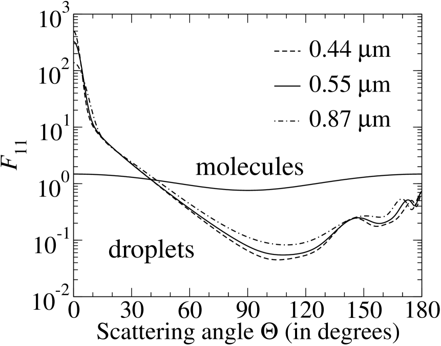
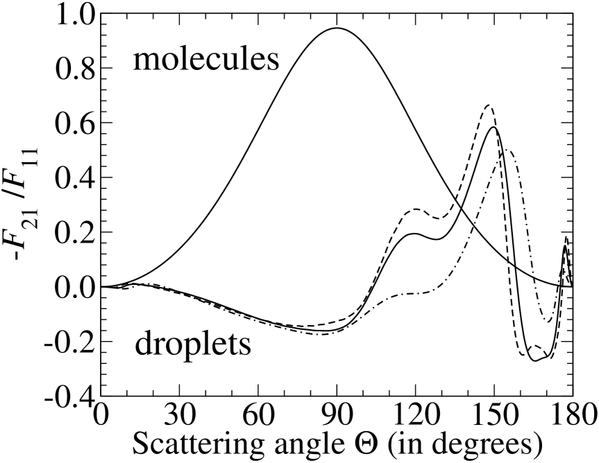
Figure 2: The phase function (scattering matrix element $F_{\rm 11}$) (on the left) and the degree of linear polarization (-$F_{\rm 21}/F_{\rm 11}$) (on the right) as functions of the scattering angle $\Theta$, for light singly scattered by gaseous molecules and cloud droplets. The wavelength of the light is 0.44 $\mu$m (dashed line, only for the cloud droplets), 0.55 $\mu$m (solid lines), and 0.87 $\mu$m (dotted line, only for the cloud droplets).

Figure 2a shows the phase functions of the gaseous molecules and the cloud droplets at $\lambda=0.55~{}\mu$m. To illustrate the wavelength dependence of the elements of the cloud droplets’ scattering matrix, we have also plotted curves for $\lambda=0.44~{}\mu$m and $\lambda=0.87~{}\mu$m (these particular wavelengths will be used again later on, in Sect. 4). For the same wavelengths, Fig. 2b shows the degree of linear polarization, $P_{\rm s}$ (Eq. 7), of light that is singly scattered by the molecules and the cloud droplets as functions of the single scattering angle, $\Theta$, assuming unpolarized incident light. The reference plane for this singly scattered light is the plane through the incoming and the scattered light beams. Note that the phase function and degree of polarization of light singly scattered by gaseous molecules depends on the wavelength, too, through the wavelength dependence of the depolarization factor (see Bates 1984), but only slightly so.

From Fig. 2, it is clear that both the phase function and the degree of polarization pertaining to single scattering by molecules vary smoothly with the single scattering angle $\Theta$. The degree of polarization, $P_{\rm s}$, of the light that is singly scattered by the molecules is positive (i.e. the direction of polarization is perpendicular to the reference plane) for all values of $\Theta$. Furthermore, $P_{\rm s}$ of this light is highest at $\Theta=90^{\circ}$. At this scattering angle, the light is not completely (i.e. 100 $\%$) polarized, but ”only” about 95 $\%$, because of the molecular depolarization factor (Bates 1984). Both for the light scattered by the molecules and for the light scattered by the cloud droplets, $P_{\rm s}$ vanishes for $\Theta=0^{\circ}$ and $\Theta=180^{\circ}$, because of symmetry.

The degree of polarization of the light scattered by the cloud droplets (Fig. 2b) changes sign (i.e. the direction of polarization changes with respect to the reference plane) a number of times between $\Theta=0^{\circ}$ and $\Theta=180^{\circ}$, and shows strong angular features, in particular in the backward scattering directions ($\Theta>90^{\circ}$). The peak in the polarization occuring at $\Theta=148^{\circ}$ for $\lambda=0.44~{}\mu$m, at $\Theta=150^{\circ}$ for $\lambda=0.55~{}\mu$m, and at $\Theta=155^{\circ}$ for $\lambda=0.87~{}\mu$m, pertains to what is commonly known as the primary rainbow, which is due to light that has been reflected inside the droplets once. The primary rainbow is seen in the flux phase functions (Fig. 2a), too, only less prominent than in $P_{\rm s}$. The angular features in $P_{\rm s}$ near $\Theta=120^{\circ}$ pertain to the secondary rainbow, which is due to light that has been reflected inside the the droplets twice. In the cloud droplets’ phase functions (Fig. 2a), only a hint of the secondary rainbow can be seen and only for $\lambda=0.44~{}\mu$m. The occurence of a rainbow in reflected light is a strong and well-known indicator for spherically shaped atmospheric particles, see e.g. Hansen & Travis (1974), and more recently Liou & Takano (2002) and references therein, and Bailey (2007).

3.2 The model surfaces

To describe the reflection of light by the homogeneous, locally flat surfaces below the atmospheres of our model planets, we have to specify the surface reflection matrix, ${\bf A}_{\rm s}$. The surface reflection matrix is normalized such that the average of matrix element (1,1) of ${\bf A}_{\rm s}$ over all reflection directions equals the surface albedo, i.e. the fraction of the incident stellar flux that the surface reflects in all directions. We’ll denote the surface albedo by $A_{\rm s}$.

The Earth’s surface is covered by numerous surface types with myriads of (wavelength dependent) albedos, many of which vary with e.g. their moistness and/or the season. To avoid making our model planets too detailed at this stage, we will compose the surfaces of our Earth-like model planets out of only two surface types: (deep) ocean and (green) vegetation. We assume that the surface that is covered by vegetation completely depolarizes all incident light, i.e. except for element element (1,1) of ${\bf A}_{\rm s}$, all elements of the vegetation’s surface reflection matrix equal zero. In addition, we assume that the reflection by the surface is isotropic, i.e. reflection matrix element (1,1) is independent of the directions of both the incoming and the reflected light; element (1,1) thus simply equals the surface albedo, $A_{\rm s}$. We thus describe a surface that is covered with vegetation as a Lambertian reflecting surface. In future studies, it will be interesting to include polarizing effects of vegetation, as presented by Wolstencroft et al. (2007).

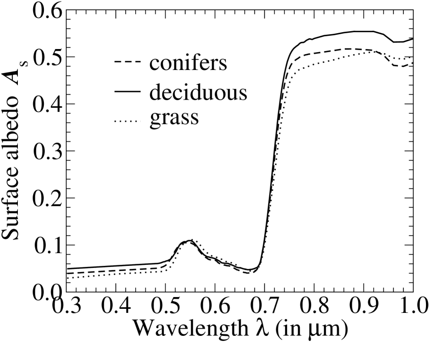
Figure 3: The measured albedos of three types of common terrestrial vegetation as functions of the wavelength: conifers (dashed line), deciduous forest (solid line), and grass (dotted line) (data from the ASTER spectral library). For our model planets, we use the albedo of deciduous forest to represent vegetated surfaces.

In Fig. 3, we have plotted measured, wavelength dependent albedos of three types of vegetation: conifers, deciduous forest, and grass These albedo spectra share the following characteristics: (1) a local maximum between 0.5 $\mu$m and 0.6 $\mu$m, that is mainly due to the presence of two absorption bands of chlorophyll, one near 0.45 $\mu$m and one near 0.67 $\mu$m, and (2) a high albedo at wavelengths longer than about 0.7 $\mu$m, that is related to the internal leaf and cell structure. The sudden increase of the surface albedo at wavelengths longer than 0.7 $\mu$m, is usually referred to as the red edge (for an elaborate description of the red edge, see Seager et al. 2005). The slight decrease in the albedo around 0.97 $\mu$m is due to absorption by water in the leaves. Stronger absorption bands of water occur at wavelengths longer than 1.2 $\mu$m. Because in this paper we do not study the effects of differences in the albedos of different types of vegetation on the light that is reflected by a planet, we will only use the wavelength dependent albedo of the deciduous forest to represent the reflectivity by vegetation on our model planets.

Whether vegetation on Earth-like extrasolar planets will have the same spectral features, in particular the red edge, as we find on Earth, is still an open question (see Wolstencroft & Raven 2002). Model studies for albedos of vegetation on Earth-like planets around M stars have been published by Kiang et al. (2007); Segura et al. (2005); Tinetti et al. (2006c). For our purpose, presenting flux and polarization spectra and in particular their differences and similarities without focussing on the detection of features, an Earth-like vegetation albedo is sufficient.

Although on Earth, deep oceans do show some color, especially in shallow regions where algae and other small organisms bloom, for the purpose of this paper it is safe to simply assume the oceans are black across the wavelength interval of our interest, i.e. from 0.3 to 1.0 $\mu$m. Even with an albedo $A_{\rm s}$ equal to zero, however, our model oceans do reflect a fraction of the light that is incident on them, because we include a specular (i.e. Fresnel) reflecting interface between the atmosphere and the black ocean. Specular reflection is anisotropic and generally leads to polarized reflected light. We use the specular reflection matrix as described by Haferman et al. (1997), with a (wavelength independent) index of refraction that is equal to 1.34. Our model ocean surface is flat, i.e. there are no waves. The influence of oceanic waves will be subject of later studies, using the wave distribution model by Cox & Munk (1954) (for a recent evaluation of this model, see Bréon & Henriot 2006), which can be included in our adding-doubling radiative transfer model (see e.g. Chowdhary et al. 2002). We neglect the contribution of whitecaps to the ocean albedo, which appears to be a valid assumption for average wind speeds measured on the Earth’s oceans (Koepke 1984).

4 Calculated flux and polarization spectra

In this section, we will present the numerically calculated total flux and degree of polarization of starlight that is reflected by Earth-like model planets as described in the previous section (Sect. 3). The reflected flux, $F$, is calculated according to Eq. 8. Unless stated otherwise, we assume that $r=1$, $d=1$, and $\pi F_{\rm 0}=1$, independent of $\lambda$. With unpolarized incident light, $F$ thus equals $\frac{1}{4}a_{\rm 1}$, which is the planet’s geometric albedo $A_{\rm G}$ in case planetary phase angle $\alpha=0^{\circ}$ (see Eq. 11). The degree of polarization is calculated according to Eq. 14, and thus includes the direction of polarization.

Tables containing elements $a_{1}$ and $b_{1}$ of the planetary scattering matrix ${\bf S}$ as functions of the wavelength, and as functions of the planetary phase angle, for the various horizontally homogeneous model planets that are presented in the following sections will be made available through the CDS. From the elements $a_{1}$ and $b_{1}$, and given distance $d$, planetary radius $r$, and the (wavelength dependent) incident stellar flux (e.g. in W m^-2 m^-1), the observable total flux, $F$, polarized flux, $Q$, and degree of polarization, $P_{\rm s}$, can be calculated using Eqs. 12, 13, and 14, respectively.

4.1 Clear planets with wavelength independent surface albedos

4.1.1 Wavelength dependence

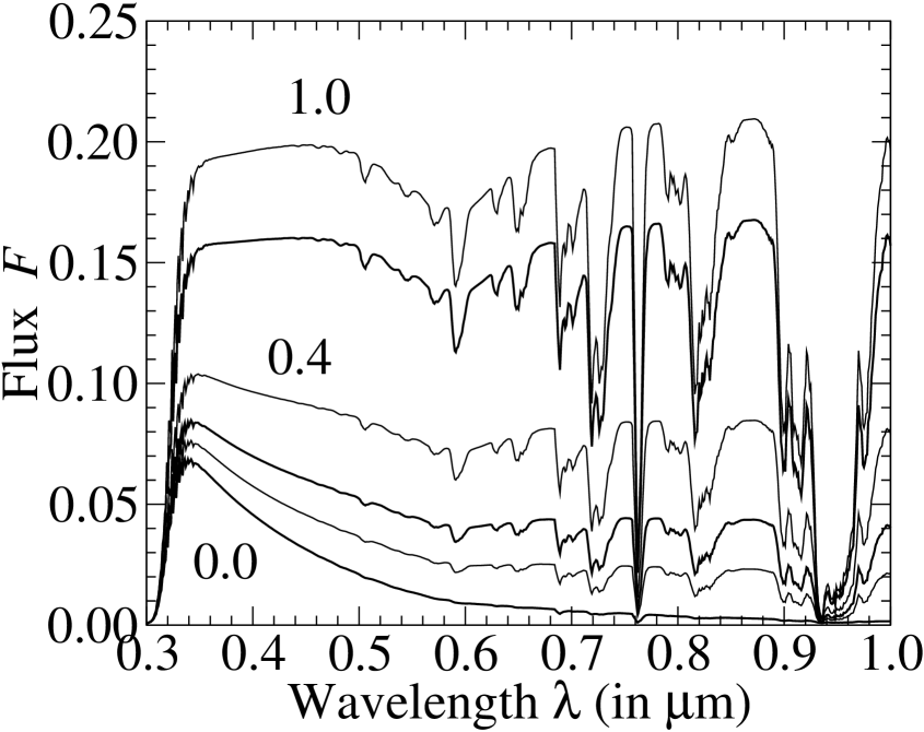
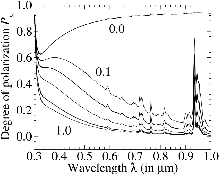
Figure 4: The flux $F$ (left) and the degree of linear polarization $P_{\rm s}$ (right) of starlight reflected by model planets with clear atmospheres and isotropically reflecting, completely depolarizing surfaces as functions of the wavelength, for various values of the (wavelength independent) surface albedo: 0.0, 0.1, 0.2, 0.4, 0.8, and 1.0. The planetary phase angle $\alpha$ is 90^∘.

Figure 4 shows the wavelength dependence of the total flux, $F$, and the degree of polarization, $P_{\rm s}$, of starlight that is reflected by six Earth–like model planets with similar, clear (i.e. cloudless) atmospheres, and Lambertian reflecting (i.e. isotropically reflecting and completely depolarizing) surfaces with wavelength independent albedos, $A_{\rm s}$, ranging from 0.0 to 1.0. The planetary phase angle, $\alpha$, is 90^∘, i.e. half of the observable planetary disk is illuminated by the star. As explained in Sect. 1, the probability to directly observe an exoplanet at or near this phase angle (quadrature) is relatively high (provided there is an observable exoplanet).

Each curve in Fig. 4 can be thought of to consist of a continuum with superimposed high–spectral resolution features. The continua of the flux and polarization curves are determined by the scattering of light by gaseous molecules in the atmosphere and by the surface albedo. The high–spectral resolution features are due to the absorption of light by the gases O₃, O₂, and H₂O (see below). Note that strength and shape of the absorption bands depend on the spectral resolution (0.001 $\mu$m) of the numerical calculations.

In the total flux curves (Fig. 4a), the contribution of light scattered by atmospheric molecules is largest around 0.34 $\mu$m; at shorter wavelengths, light is absorbed by O₃ in the so-called Huggins absorption band, and at longer wavelengths, the amount of starlight that is scattered by the atmospheric molecules decreases, simply because the atmospheric molecular scattering optical thickness decreases with wavelength, as $b^{\rm m}_{\rm sca}$ is roughly proportional to $\lambda^{-4}$ (see e.g. Stam et al. 2000a). For the planet with the black surface ($A_{\rm s}=0.0$), where the only light that is reflected by the planet comes from scattering by atmospheric molecules, the flux of reflected starlight decreases towards zero with increasing wavelength. For the planets with reflecting surfaces, the contribution of light that is reflected by the surface to the total reflected flux increases with increasing wavelength. Because the surface albedos are wavelength independent, the continua of the reflected fluxes become wavelength independent, too, at the longest wavelengths. This is not obvious from Fig. 4a, because of the presence of high-spectral resolution features.

The high–spectral resolution features in the flux curves of Fig. 4 are all due to gaseous absorption bands. As mentioned above, at the shortest wavelengths, light is absorbed by O₃. The so–called Chappuis absorption band of O₃ gives a shallow depression in the flux curves that is visible between about 0.5 $\mu$m and 0.7 $\mu$m, in particular in the curves pertaining to a high surface albedo. The flux curves contain four absorption bands of O₂, i.e. the $\gamma$-band around 0.63 $\mu$m, the $B$-band around 0.69 $\mu$m, the conspicuous $A$-band around 0.76 $\mu$m, and a weak band around 0.86 $\mu$m. These absorption bands, except the $A$-band, are difficult to identify from Fig. 4a, because they are located either next to or within one of the many absorption bands of H₂O (which are all the bands not mentioned previously).

The polarization curves (Fig. 4b) are, like the flux curves, shaped by light scattering and absorption by atmospheric molecules, and by the surface reflection. The contribution of the scattering by atmospheric molecules is most obvious for the planet with the black surface ($A_{\rm s}=0.0$), where there is no contribution of the surface to the reflected light. For this model planet and phase angle, $P_{\rm s}$ has a local minimum around 0.32 $\mu$m. At shorter wavelengths, $P_{\rm s}$ is relatively high because there the absorption of light in the Huggins band of O₃ decreases the amount of multiple scattered light, which usually has a lower degree of polarization than the singly scattered light. In general, with increasing atmospheric absorption optical thickness, $P_{\rm s}$ will tend towards the degree of polarization of light singly scattered by the atmospheric constituents (for these model planets: only gaseous molecules), which depends strongly on the single scattering angle $\Theta$ and thus on the planetary phase angle $\alpha$. From Fig. 2b, it can be seen that at a scattering angle of 90^∘, $P_{\rm s}$ of light singly scattered by gaseous molecules is about 0.95. This explains the high values of $P_{\rm s}$ at the shortest wavelengths in Fig. 4b. With increasing wavelength, the amount of multiple scattered light decreases, simply because of the decrease of the atmospheric molecular scattering optical thickness. Consequently, $P_{\rm s}$ of the planet with the black surface increases with wavelength, to approach its single scattering value at the smallest scattering optical thicknesses.

With a reflecting surface below the atmosphere, $P_{\rm s}$ also tends to its single scattering value at the shortest wavelengths, because with increasing atmospheric absorption optical thickness, the contribution of photons that have been reflected by the depolarizing surface to the total number of reflected photons decreases (both because with absorption in the atmosphere, less photons reach the surface and less photons that have been reflected by the surface reach the top of the atmosphere) (see e.g. Stam et al. 1999). In case the planetary surface is reflecting, $P_{\rm s}$ of the planet will start to decrease with wavelength, as soon as the contribution of photons that have been reflected by the depolarizing surface to the total number of reflected photons becomes significant. As can been seen in Fig. 4b, the wavelength at which the decrease of $P_{\rm s}$ starts depends on the surface albedo: the higher the albedo, the shorter this wavelength. It is also obvious that with increasing wavelength, the sensitivity of $P_{\rm s}$ to $A_{\rm s}$ decreases. This sensitivity clearly depends on the atmospheric molecular scattering optical thickness.

Like with the flux curves, the high–spectral resolution features in the polarization curves of Fig. 4b are all due to gaseous absorption. The explanation for the increased degree of polarization inside the O₂ and H₂O absorption bands is the same as that given above for the Huggins absorption band of O₃: with increasing atmospheric absorption optical thickness, the contribution of multiple scattered light to the reflected light decreases, and hence $P_{\rm s}$ increases towards the degree of polarization of light singly scattered by the atmospheric constituents, i.e. gaseous molecules. In case atmospheres contain aerosol and/or cloud particles, $P_{\rm s}$ both inside and outside the absorption bands will depend on the single scattering properties of those aerosol and/or cloud particles, too (see Stam et al. 1999, for a detailed description of $P_{\rm s}$ across gaseous absorption lines). Stam et al. (2004) and Stam (2003) show calculated polarization spectra of Jupiter-like extrasolar planets with gaseous absorption bands due to methane. An increase of the degree of polarization across gaseous asorption bands has been measured in so–called zenith sky observations on Earth (Stammes et al. 1994; Preusker et al. 1995; Aben et al. 1997, 1999), and, recently, in observations of Jupiter, Uranus and Neptune (Joos & Schmid 2007; Schmid et al. 2006; Joos et al. 2005), with methane as the absorbing gas.

It is interesting to note that the polarization spectrum of an extrasolar planet will generally be insensitive to absorption that takes place between the planet and the observer because it is a relative measure (see Eqs. 6 and 7). Thus, if the telescope were located on the Earth’s surface, the polarization features as shown in Fig. 4b would be unaffected by absorption within the Earth’s atmosphere; polarimetry would in principle allow the detection of e.g. O₂ in an extrasolar planetary atmosphere despite the O₂ in the Earth’s atmosphere (the number of photons received by the telescope, i.e. the flux, would of course be strongly affected by absorption in the Earth’s atmosphere).

4.1.2 Phase angle dependence

Figure 5 shows the phase angle dependence of the total flux, $F$, and the degree of polarization, $P_{\rm s}$, of the starlight that is reflected by three of the six Earth-like planets appearing in the previous section, namely, the planets with $A_{\rm s}=0.0$, 0.4, and 1.0. The phase angle dependence has been plotted for two wavelengths: 0.44 $\mu$m and 0.87 $\mu$m. Remember that the flux at phase angle $\alpha=0^{\circ}$ is just the planet’s geometric albedo $A_{\rm G}$ (Eq. 11). For $A_{\rm s}=0.0$, $A_{\rm G}=0.14$ at $\lambda=0.44~{}\mu$m, and $A_{\rm G}=0.011$ at $\lambda=0.87~{}\mu$m. For $A_{\rm s}=0.4$ and 1.0, we find, respectively, $A_{\rm G}=0.34$ (0.44 $\mu$m) and 0.27 (0.87 $\mu$m), and 0.72 (0.44 $\mu$m) and 0.67 (0.87 $\mu$m) (see Fig. 5a). The planets’ geometric albedos at $\lambda=0.87~{}\mu$m are close to $\frac{2}{3}\hskip 2.27626ptA_{\rm s}$, i.e. the geometric albedo of a planet with a Lambertian reflecting surface but without an atmosphere (see Stam et al. 2006), because at this wavelength, the scattering optical thickness of the model atmosphere is only 0.015. At 0.44 $\mu$m, this optical thickness is 0.24, and the light scattered within the model atmosphere does contribute significantly to the planet’s geometric albedo, especially when $A_{\rm s}$ is small.

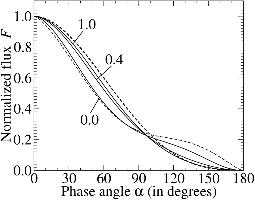
Figure 6: The fluxes of Fig. 5a, normalized to 1.0 at $\alpha=0^{\circ}$. For $\lambda=0.87~{}\mu$m (dashed lines), the curves for $A_{\rm s}=1.0$ and $A_{\rm s}=0.4$ are virtually indistinguishable, and follow the theoretical (normalized) curve expected for a Lambertian reflecting sphere (see van de Hulst 1980; Stam et al. 2006), i.e. $F(\alpha)=\frac{1}{\pi}\left(\sin\alpha+(\pi-\alpha)\cos\alpha\right)$, with $\alpha$ in radians.

The strong phase angle dependence of $F$ (Fig. 5a) is, for a given value of $A_{\rm s}$, largely due to the variation of the illuminated and visible fraction of the planetary disk with the phase angle. Other variations are related to the reflection properties of the surface and the scattering properties of the overlying atmosphere. These variations can be seen more clearly in Fig. 6, where we show the curves of Fig. 5a normalized at $\alpha=0^{\circ}$. The curves for $\lambda=0.87~{}\mu$m and $A_{\rm s}=0.4$ and $A_{\rm s}=1.0$ coincide with the theoretical (normalized) curve expected for Lambertian reflecting spheres (see van de Hulst 1980; Stam et al. 2006), because, as explained above, at this wavelength, the contribution of light scattered within the model atmosphere is almost negligible.

In Fig. 5b, we show the degree of polarization, $P_{\rm s}$, as a function of the phase angle. Like the reflected flux, $P_{\rm s}$ depends strongly on the phase angle. Note that for $\alpha=0^{\circ}$ and $\alpha=180^{\circ}$, $P_{\rm s}$ equals zero because of symmetry (the incoming starlight is unpolarized). For the planet with the black surface, $P_{\rm s}$ appears to be fairly symmetric around $\alpha=90^{\circ}$, mainly because the degree of polarization of light singly scattered by gaseous molecules is symmetric around $\Theta=90^{\circ}$ (see Fig. 2b). This symmetry is particularly apparent for $\lambda=0.87~{}\mu$m, where there is much less multiple scattering than for $\lambda=0.44~{}\mu$m. Across most of the phase angle range, $P_{\rm s}$ of the planet with the black surface is positive, indicating that the reflected light is polarized perpendicular to the scattering plane (i.e. perpendicular to the imaginary line connecting the planet and the star as seen by the observer). Only for the largest scattering angles, $P_{\rm s}~{}<~{}0$ (which is difficult to see in Fig. 5b for $\lambda=0.87~{}\mu$m). At these angles, the reflected light is thus polarized parallel to the scattering plane (i.e. parallel to the imaginary line connecting the planet and the star). The negative polarization is mainly due to second order scattered light: although this light comprises only a small fraction of the reflected light at these large phase angles, it does leave its traces in the polarization signature of the planet, because the degree of polarization of the first order scattered light (which is the main contributor to the reflected light) is close to zero. For $\lambda=0.44~{}\mu$m, $P_{\rm s}<0$ when $\alpha>164^{\circ}$, while for $\lambda=0.87~{}\mu$m, $P_{\rm s}<0$ only when $\alpha>174^{\circ}$, because with increasing wavelength, the amount of second order scattered light decreases, and with that the phase angle at which the second order scattered light changes the sign of $P_{\rm s}$ increases.

For the planets with the reflecting surfaces, the maximum degree of polarization occurs at phase angles larger than 90^∘ (see Fig. 5b). In particular, with increasing wavelength and/or increasing surface albedo, the maximum degree of polarization shifts to larger phase angles, because with increasing $\alpha$, the fraction of reflected light that has touched the depolarizing surface at least once, decreases. The contribution of light that has been polarized within the planetary atmosphere to the reflected light thus increases with increasing $\alpha$. This also explains why at the largest values of $\alpha$, $P_{\rm s}$ in Fig. 5b, is independent of $A_{\rm s}$.

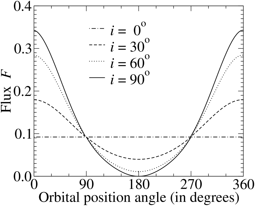
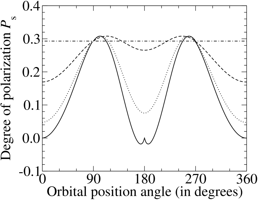
Figure 7: $F$ (left) and $P_{\rm s}$ (right) of starlight with $\lambda=0.44~{}\mu$m that is reflected by the model planet with $A_{\rm s}=0.4$ as functions of the orbital position angle for the following orbital inclination angles $i$: 0^∘ (dot-dashed lines), 30^∘ (dashed lines), 60^∘ (dotted lines), and 90^∘ (solid lines).

Figure 7 shows $F$ and $P_{\rm s}$ as functions of the planet’s orbital position angle for orbital inclination angles, $i$, ranging from 0^∘ (the orbit is seen face–on) to 90^∘ (the orbit is seen edge–on). Given an inclination angle $i$, an exoplanet can in principle be observed at phase angles, $\alpha$, ranging from $90^{\circ}-i$ to $90^{\circ}+i$. If the orbital position angle equals 0^∘ or 360^∘, $\alpha$ ranges from 90^∘ ($i=0^{\circ}$) to 0^∘ ($i=90^{\circ}$). If the orbital position angle equals 90^∘ or 270^∘, the planetary phase angle, $\alpha$, equals 90^∘ (independent of $i$). If the orbital position angle equals 180^∘, $\alpha$ ranges from 90^∘ ($i=0^{\circ}$) to 180^∘ ($i=90^{\circ}$). The curves in Fig. 7 clearly show that with increasing orbital inclination angle, the variation of $F$ and $P_{\rm s}$ along the planetary orbit increases. Interestingly, the orbital position angles where a planet is easiest to observe directly because it is furthest from its star (in angular distance) are those where $P_{\rm s}$ is largest (namely, at orbital position angles equal to 90^∘ and 270^∘) This emphasizes the strength of polarimetry for extrasolar planet detection and characterization. Incidentally, $P_{\rm s}$ is smallest for the inclination angles and orbital position angles where it is the most difficult or even impossible to directly observe the planet, i.e. at large inclination angles and orbital position angles equal to 0^∘, 180^∘, or 360^∘, when the planet is close to, or even in front of or behind its star.

4.2 Clear and cloudy planets with wavelength dependent surface albedos

4.2.1 Wavelength dependence

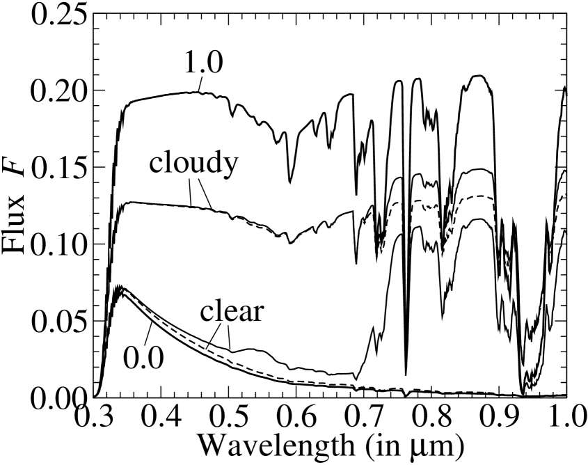
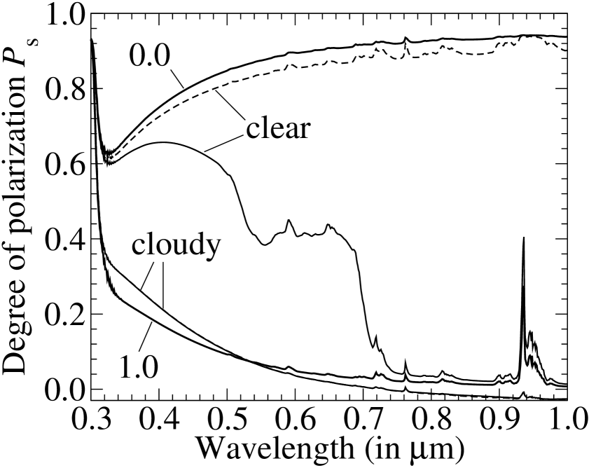
Figure 8: The wavelength dependent flux, $F$, (left) and degree of polarization, $P_{\rm s}$, (right) of starlight that is reflected by clear and cloudy horizontally homogeneous model planets with surfaces covered by deciduous forest (thin solid lines), a specular reflecting ocean (thin dashed lines). Note that the lines pertaining to $P_{\rm s}$ of the cloudy atmospheres are virtually indistinguishable from each other. For comparison, we have also included the spectra of the clear model planets with surface albedos equal to 0.0 and 1.0 (thick solid lines), shown before in Fig. 4. The planetary phase angle, $\alpha$, is 90^∘.

Figure 8 shows the wavelength dependence of the total flux, $F$, and degree of polarization, $P_{\rm s}$, of starlight that is reflected by planets that are completely covered by, respectively, ocean and deciduous forest, with atmospheres that are either clear, i.e. cloudless, or cloudy, i.e. that contain a homogeneous cloud layer. The cloud and the cloud particles have been described in Sect. 3.1. For comparison, we have also plotted $F$ and $P_{\rm s}$ of the clear white and black planets discussed in Sect. 4.1. The planetary phase angle, $\alpha$, is 90^∘. First, we will discuss $F$ and $P_{\rm s}$ of the planets with the clear atmospheres, and then those of the cloudy planets.

The surface albedo of the clear planet that is covered by ocean equals zero, regardless of wavelength (see Sect. 3.2). The differences between $F$ and $P_{\rm s}$ of the clear black planet and $F$ and $P_{\rm s}$ of the clear, ocean covered planet (see Fig. 8), are thus due to the specular reflecting interface between the model atmosphere and the ocean, which increases the total amount of light that is reflected back towards the observer. In Fig. 8a, the specular reflection increases $F$ in the continuum with about 10$\%$ at the short wavelengths and with about 20$\%$ at the long wavelengths (where more incoming starlight reaches the surface, because of the smaller atmospheric optical thickness). Although very difficult to see in Fig. 8a, the influence of the specular reflection on $F$ is small within the gaseous absorption bands, because at those wavelengths, little light reaches the surface and after a reflection there, the top of the atmosphere again.

As can be seen in Fig. 8b, the specular reflection decreases $P_{\rm s}$ in the continuum with a few percentage points, because with the specular reflection, a fraction of the light that is incident on the surface is reflected back towards the atmosphere, adding mainly to the unpolarized flux (at least at this phase angle). In gaseous absorption bands, the influence of the specular reflection on $P_{\rm s}$ is smaller than in the continuum, because at these wavelengths less light reaches the surface and after a reflection there, the top of the atmosphere again.

The wavelength variation of the continuum $F$ and $P_{\rm s}$ pertaining to the clear, forest–covered planet reflects the wavelength variation of the surface albedo (see Fig. 3) except at the shortest wavelengths. There, $F$ and $P_{\rm s}$ are mainly determined by the light that has been scattered by the gaseous molecules within the planet’s atmosphere, because (1) the atmospheric scattering optical thickness increases with decreasing wavelength, and (2) the surface albedo is only about 0.05 at the shortest wavelengths (see Fig. 3). At longer wavelengths, the characteristic reflection by chlorophyll (around 0.54 $\mu$m) and the red edge (longwards of 0.7 $\mu$m) can easily be recognized both in $F$ and in $P_{\rm s}$. The red edge in flux spectra of the Earth has been detected by instruments onboard the Galileo mission on its way to Jupiter (Sagan et al. 1993), and from the ground it has been observed and in some cases modeled by different research groups (see e.g. Hamdani et al. 2006; Montañés-Rodríguez et al. 2006; Tinetti et al. 2006b, a; Seager et al. 2005; Woolf et al. 2002; Arnold et al. 2002) in spectra of Earthshine, the sunlight that has first been reflected by the Earth and then by the moon, and that can be observed on the moon’s nightside. Interestingly, the reflection by chlorophyll leaves a much stronger signature in $P_{\rm s}$ than in $F$, because in this wavelength region $P_{\rm s}$ appears to be very sensitive to small changes in $A_{\rm s}$, as can also be seen in Fig. 4b.

Adding a cloud layer to the atmosphere of a planet covered with either vegetation or ocean, increases $F$ across the whole wavelength interval (see Fig. 8a). A discussion on the effects of different types of clouds on flux spectra of light reflected by exoplanets is given by Tinetti et al. (2006b, a). Our simulations show that although the cloud layers of the two cloudy planets have a large optical thickness (i.e. 10 at $\lambda=0.55$ $\mu$m, as described in Sect. 3.1) both cloudy planets in Fig. 8a are darker than the white planet with the clear atmosphere (the flux of which is also plotted in Fig. 8a). The cloud particles themselves are only slightly absorbing (see Sect. 3.1). Apparently, on the cloudy planets, a significant amount of incoming starlight is diffusely transmitted through the cloud layer (through multiple scattering of light) and then absorbed by the planetary surface (the albedos of the ocean and the forest are smaller than 1.0). Thus, even with an optically thick cloud, the albedo of the planetary surface still influences the light that is reflected by the planets, and approximating clouds by isotropically or anisotropically reflecting surfaces, without regard for what is underneath, as is sometimes done (see e.g. Montañés-Rodríguez et al. 2006; Woolf et al. 2002) is not appropriate. Assuming a dark surface beneath scattering clouds with non-negligible optical thickness (Tinetti et al. 2006b, a) will lead to too dark planets. The influence of the surface albedo is in particularly clear for the cloudy planet that is covered with vegetation: longwards of 0.7 $\mu$m, the continuum flux of this planet still shows the vegetation’s red edge. The visibility of the red edge through optically thick clouds strengthens the detectability of surface biosignatures in the visible wavelength range as discussed by (Tinetti et al. 2006b), whose numerical simulations showed that, averaged over the daily time scale, Earth’s land vegetation would be visible in disk-averaged spectra, even with cloud cover, and even without accounting for the red edge below the optically thick clouds. Note that the vegetation’s albedo signature due to chlorofyll, around 0.54 $\mu$m, also shows up in Fig. 8a, but hardly distinguishable.

The degree of polarization, $P_{\rm s}$, of the cloudy planets is low compared to that of planets with clear atmospheres, except at short wavelengths. The reasons for the low degree of polarization of the cloudy planets are (1) the cloud particles strongly increase the amount of multiple scattering of light within the atmosphere, which decreases the degree of polarization, (2) the degree of polarization of light that is singly scattered by the cloud particles is generally lower than that of light singly scattered by gaseous molecules, especially at single scattering angles around 90^∘ (see Fig. 2b), and (3) the direction of polarization of light singly scattered by the cloud particles is opposite to that of light singly scattered by gaseous molecules (see Fig. 2b). Thanks to the latter fact, the continuum $P_{\rm s}$ of the cloudy planets is negative (i.e. the direction of polarization is perpendicular to the terminator) at the longest wavelengths (about -0.03 or 3 $\%$ for $\lambda>0.73~{}\mu$m in Fig. 8b). At these wavelengths, the atmospheric molecular scattering optical thickness is negligible compared to the optical thickness of the cloud layer, and therefore almost all of the reflected light has been scattered by cloud particles.

Unlike in the flux spectra, the albedo of the surface below a cloudy atmosphere leaves almost no trace in $P_{\rm s}$ of the reflected light: the red edge of the vegetation hardly leads to a difference between $P_{\rm s}$ of the cloudy planets (Fig. 8b). In particular, at 1.0 $\mu$m, $P_{\rm s}$ of the cloudy, vegetation–covered planet is -0.030 (-3.0$\%$), while $P_{\rm s}$ of the cloudy, ocean–covered planet is -0.026 (-2.6$\%$). The reason of the insensitivity of $P_{\rm s}$ of these two cloudy planets to the surface albedo is that the light reflected by the surfaces in our models adds mainly unpolarized light to the atmosphere, in a wavelength region where $P_{\rm s}$ is already very low because of the clouds.

The cloud layer has interesting effects on the strengths of the absorption bands of O₂ and H₂O both in $F$ and in $P_{\rm s}$: because the cloud particles scatter light very efficiently, their presence strongly influences the average pathlength of a photon within the planetary atmosphere. At wavelengths where light is absorbed by atmospheric gases, clouds thus strongly change the fraction of light that is absorbed, and with that the strength of the absorption band. These are well-known effects in Earth remote-sensing; in particular the O₂ $A$-band is used to derive e.g. cloud top altitudes and/or cloud coverage within a ground pixel (see e.g. Kuze & Chance 1994; Fischer & Grassl 1991; Fischer et al. 1991; Saiedy et al. 1967; Stam et al. 2000b), because oxygen is well-mixed within the Earth’s atmosphere. In general, clouds will decrease the relative depth (i.e. with respect to the continuum) of absorption bands in reflected flux spectra (see Fig. 8a), because they shield the absorbing gases that are below them. However, because of the multiple scattering within the clouds, the absorption bands will be deeper than expected when using a reflecting surface to mimic the clouds. For example, the discrepancy between absorption band depths in Earth-shine flux observations and model simulations as shown by Montañés-Rodríguez et al. (2006), with the observation yielding e.g. a deeper O₂-A band than the model can fit, can be due to neglecting (multiple) scattering within the clouds, as Montañés-Rodríguez et al. (2006) themselves also remark.

Another source for differences between absorption band depths in observed and modeled flux spectra could be that when modeling albedo and/or flux spectra, the state of polarization of the light is usually neglected. Stam & Hovenier (2005) showed for Jupiter-like extrasolar planets that neglecting polarization can lead to errors of up to 10 $\%$ in calculated geometric albedos, and that in particular the depths of absorption bands are affected, because the error in the continuum is usually much larger than the error in the deepest part of the absorption band. In Sect. 5, we will show that neglecting polarization does not significantly change the depth of the absorption bands in the flux spectra of these Earth-like model planets.

In the polarization spectra (Fig. 8b), the effects of clouds on the strength of the absorption band features are more complicated than in flux spectra, because the absorption not only changes the amount of multiple scattering that takes place in the atmosphere, but also the altitude where the reflected light has obtained its state of polarization; in an inhomogeneous atmosphere, like a cloudy one, different particles at different altitudes can leave the light they scatter in different states of polarization (this also affects the scattered fluxes, but less so) (see e.g. Stam et al. 1999). In Fig. 8b, $P_{\rm s}$ slightly increases within absorption bands in wavelength regions where the continuum $P_{\rm s}$ is positive ($\lambda<0.73~{}\mu$m), whereas $P_{\rm s}$ slightly decreases (in absolute sense) within absorption bands in wavelength regions where the continuum $P_{\rm s}$ is negative ($\lambda>0.73~{}\mu$m). In these cloudy model atmospheres, both the increase and the decrease (in absolute sense) of $P_{\rm s}$ in absorption bands are due to (1) a decrease of multiple scattering (which also takes place in purely gaseous model atmospheres), and (2) an increase of the relative amount of photons that are scattered by gaseous molecules instead of by cloud particles, since the latter are located in the lower atmospheric layers.

The change of the strength of an absorption band in $F$ or $P_{\rm s}$ due to the presence of a cloud layer, depends strongly on the altitude of the cloud layer, its optical thickness, the cloud coverage , the mixing ratio and the vertical distribution of the absorbing gas. For example, in both the flux and the polarization spectra of the cloudy planets in Fig. 8, the absorption bands of H₂O are weak compared to the same bands in the spectra of the cloudless planets, because most of the H₂O is located below the clouds. The absorption bands of O₂ are also weaker for the cloudy planets than for the cloudless planets, although the influence of the clouds on these absorption bands is less strong than on the bands of H₂O, simply because O₂ is well–mixed throughout the atmosphere, and thus not primarily located below the clouds, like H₂O.

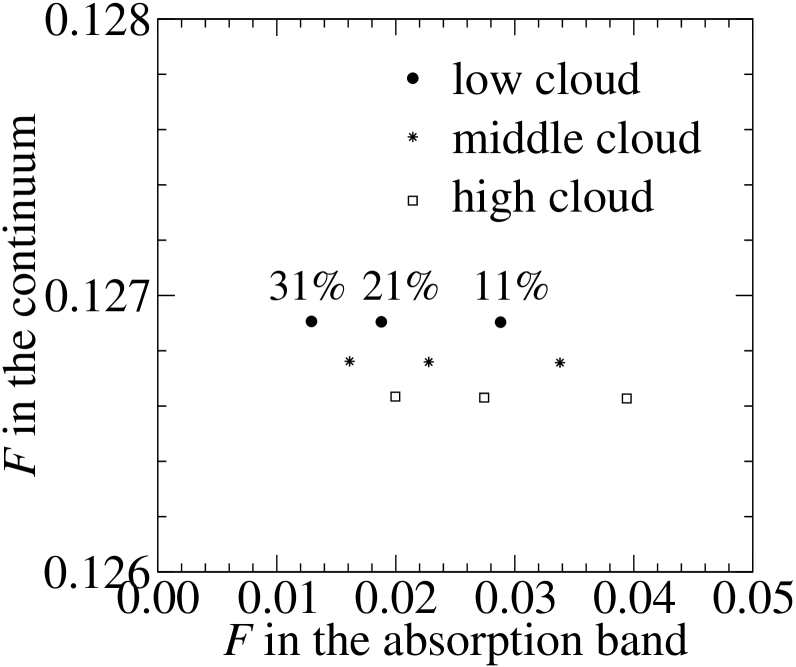
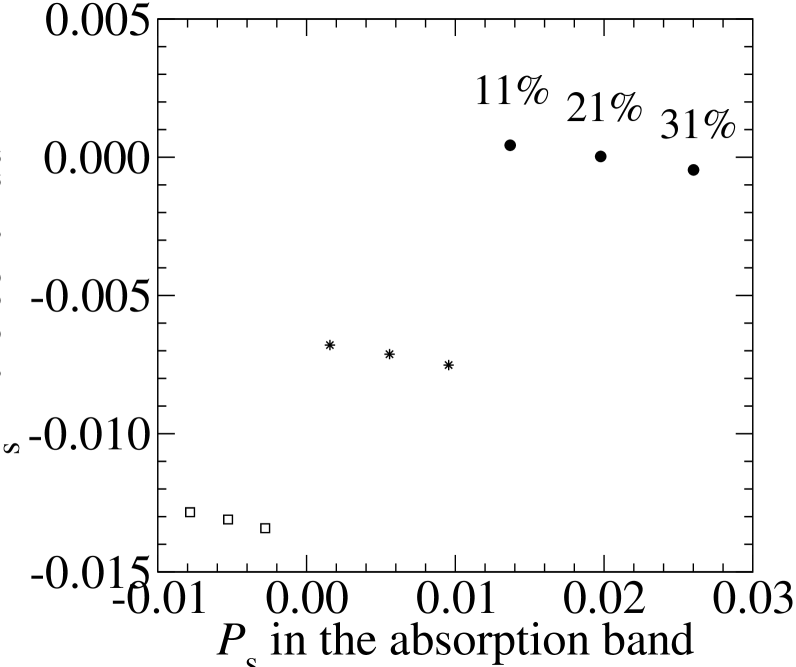
Figure 9: The flux $F$ (left) and the degree of linear polarization $P_{\rm s}$ (right) of starlight reflected by cloudy ocean planets, at $\lambda=0.762~{}\mu$m, with absorption by O₂ (along the $x$-axes) and without absorption by O₂ (along the $y$-axes). The top of the cloud layer was located at 802 hPa (the ’low cloud’; the nominal altitude), 628 hPa (the ’middle cloud’), or 487 hPa (the ’high cloud’). The O₂ mixing ratio was 11$\%$, 21$\%$ (the nominal value), or 31$\%$. The planetary phase angle $\alpha$ is 90^∘.

When a terrestrial type extrasolar planet will be discovered, it will of course be extremely interesting to try to identify oxygen in the planet’s atmosphere, and in particular to determine the oxygen mixing ratio from absorption bands such as the O₂ $A$-band. As discussed above, the depth of such an absorption band will depend not only on the absorber’s mixing ratio, but also on the cloud cover. As an example, Fig. 9 shows the influence of the cloud top altitude and the O₂ mixing ratio on the depth of the O₂-$A$ absorption band, both for the flux and the degree of polarization of the reflected starlight, for $\alpha=90^{\circ}$. The figure shows the results of numerical calculations for model planets covered by ocean and with cloud layers of optical thickness 10 (at 0.55 $\mu$m) placed with their tops at, respectively, 802 hPa, 628 hPa, and 487 hPa, and with oxygen mixing ratios of, respectively, 11 $\%$, 21 $\%$, and 31 $\%$. From Fig. 9a, it is clear that the continuum flux is independent of the O₂ mixing ratio, as it should be, and that it is virtually independent of the cloud top altitude (note the vertical scale). The latter is easily understood by realizing that at these wavelengths, the gaseous molecular scattering optical thickness above the different cloud layers is negligible compared to the scattering optical thickness of the cloud layers themselves. Not surprisingly, the flux in the absorption band increases significantly with a decreasing O₂ mixing ratio and with increasing cloud top altitude (i.e. decreasing cloud top pressure). Concluding, the depth of the O₂ $A$–band in planetary flux spectra depends on the O₂ mixing ratio as well as on the cloud top altitude, and it can thus not be used for deriving the O₂ mixing ratio if the cloud top altitude is unknown or vice versa. Figure 9b shows the relation between $P_{\rm s}$ in the continuum and in the absorption band, and the cloud top altitude and oxygen mixing ratio. Apparently, the continuum $P_{\rm s}$ depends significantly on the cloud top altitude, because the degree of polarization is very sensitive to even small amounts of gaseous molecules, and depends only very slightly on the oxygen mixing ratio. The degree of polarization in the absorption band depends on the oxygen mixing ratio as well as on the cloud top altitude. Concluding, the strength of the O₂ $A$ band in planetary polarization spectra can be used to derive both the cloud top altitude and the oxygen mixing ratio. The influence of e.g. broken cloud layers, and clouds at different altitudes on $F$ and $P_{\rm s}$, will be subject for later studies.

4.2.2 Phase angle dependence

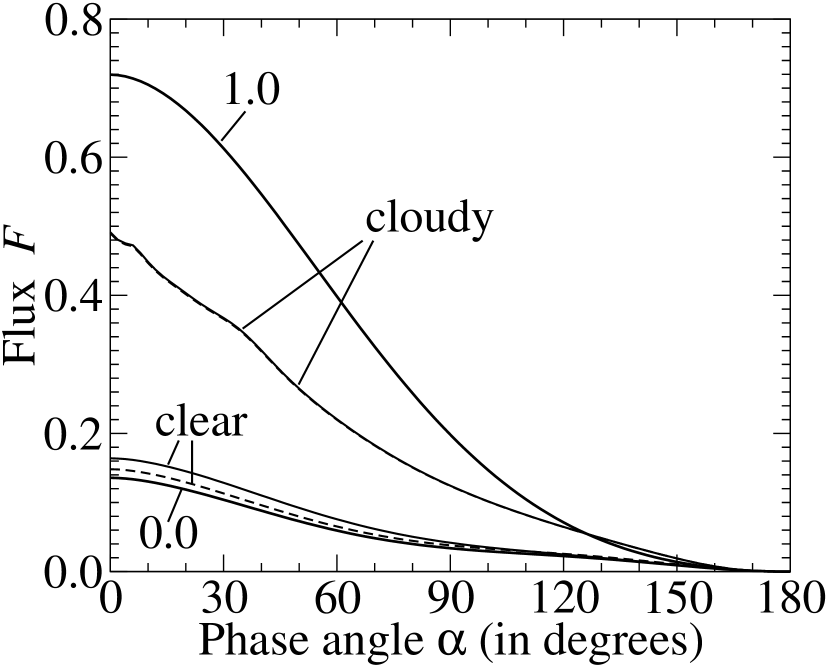
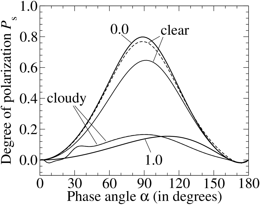
Figure 10: The flux $F$ (left) and the degree of linear polarization $P_{\rm s}$ (right) of starlight reflected by the model planets of Fig. 8 as functions of the phase angle $\alpha$, for $\lambda=0.44$ $\mu$m. The thin solid line pertains to the vegetation–covered planet, and the thin dashed line to the ocean–covered planet. The lines pertaining to the cloudy planets are virtually indistinguishable from each other.

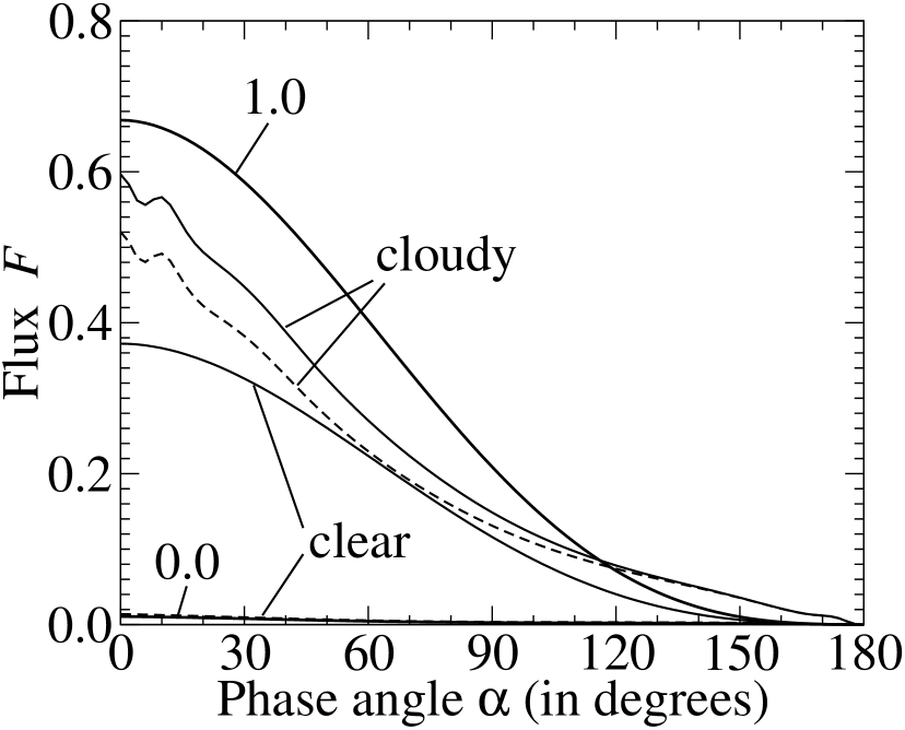
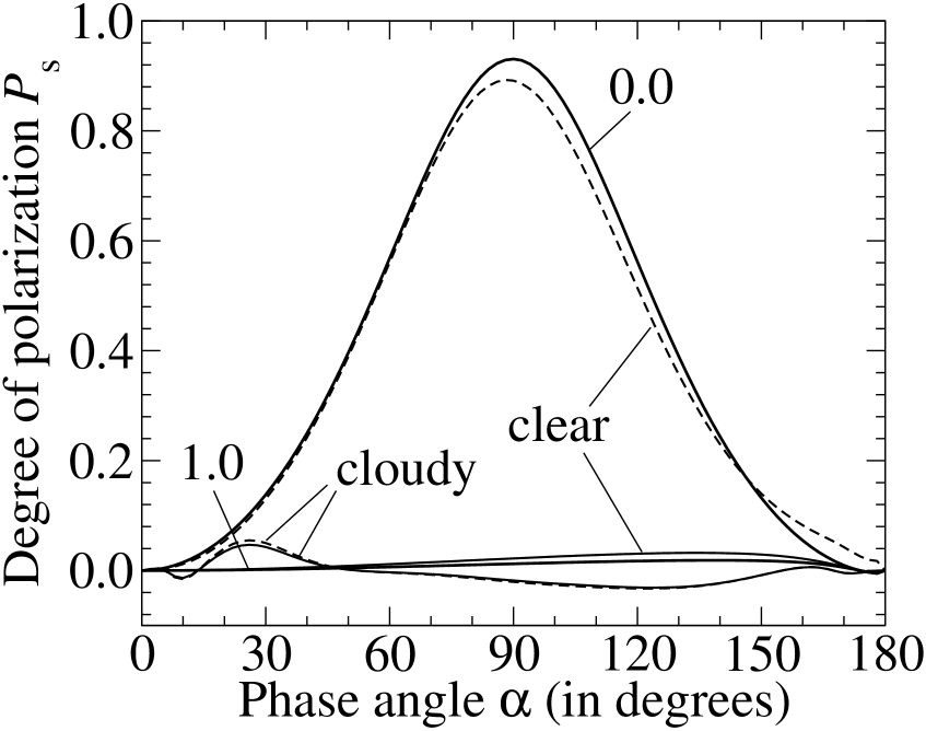
Figure 11: Same as Fig. 10, except for $\lambda=0.87$ $\mu$m. The lines for $P_{\rm s}$ pertaining to the cloudy planets are virtually indistinguishable from each other, except at phase angles between 20^∘ and 40^∘.

Figures 10 and 11 show the phase angle dependence of $F$ and $P_{\rm s}$ of the starlight that is reflected by the clear and cloudy, ocean and vegetation–covered planets appearing in the previous section (see Sect. 4.2.1 and Fig. 8) at $\lambda=0.44~{}\mu$m (Fig. 10) and at $\lambda=0.87~{}\mu$m (Fig. 11), respectively. Remember that at phase angle $\alpha=0^{\circ}$, the fluxes plotted in Figs. 10a and 11a are just the planets’ geometric albedos, $A_{\rm G}$, at those wavelengths. For the clear, ocean–covered planet, $A_{\rm G}$ is 0.15 at $\lambda=0.44~{}\mu$m, and 0.014 at $0.87~{}\mu$m. For the clear, vegetation–covered planet, $A_{\rm G}$ is 0.16 at $0.44~{}\mu$m, and 0.37 at $0.87~{}\mu$m. For the cloudy, ocean–covered planet, $A_{\rm G}$ is 0.49 at $0.44~{}\mu$m, and 0.52 at $0.87~{}\mu$m, and for the cloudy, vegetation–covered planet, $A_{\rm G}$ is 0.49 at $0.44~{}\mu$m (like for the cloudy, ocean–covered planet), and 0.60 at $0.87~{}\mu$m.

For the two cloudy planets, the reflected flux is not a smoothly decreasing function of phase angle, but instead shows some bumpy features near $\alpha=5^{\circ}$ and 30^∘ for $\lambda=0.44~{}\mu$m (Fig. 10a), and near 10^∘ and 35^∘ for $\lambda=0.87~{}\mu$m (Fig. 11a). These angular features trace back to features in the single scattering phase function of the cloud particles (at scattering angles, $\Theta$, larger than 140^∘) (see Fig. 2a). Because at $\lambda=0.44~{}\mu$m, the gaseous molecules above the cloud layer scatter light more efficiently than at $\lambda=0.87~{}\mu$m, the angular features in $F$ are more subdued at 0.44 $\mu$m than at 0.87 $\mu$m. Interestingly, at phase angles near 60^∘ and for $\lambda=0.87~{}\mu$m (Fig. 11a), the cloudy, ocean–covered planet is about as bright as the clear, vegetation–covered planet. Apart from the high surface albedo of the vegetation at this wavelength (Fig. 3), this can partly be attributed to the single scattering phase function of the cloud particles, too, because this function has a broad minimum between $\Theta=90^{\circ}$ and $\Theta=120^{\circ}$ (see Fig. 2a). Note further that only at the largest phase angles, i.e. $\alpha>120^{\circ}$, the cloudy planets are brighter than the clear planet with the surface albedo equal to 1.0. This is in particularly obvious at $\lambda=0.87~{}\mu$m (Fig. 11a), and is due to the strong forward scattering peak in the single scattering phase functions of the cloud particles (Fig. 2a). At these large phase angles, the light that is reflected by the cloudy planets has not reached the surface, and the reflected flux is therefore independent of the surface albedo (see Fig. 11a).

The phase angle dependence of the degree of linear polarization, $P_{\rm s}$, of the light reflected by the two cloudy planets (Figs. 10b and 11b) shows, for $\alpha<40^{\circ}$, angular features that are due to angular features in the single scattering polarization phase function of the cloud particles (see Fig. 2b), just like the phase angle dependence of the reflected flux (Figs. 10a and 11a). At $\lambda=0.44~{}\mu$m, $P_{\rm s}$ is determined not only by light scattered by the cloud particles, but also by light scattered by the gaseous molecules, whereas at $\lambda=0.87~{}\mu$m, $P_{\rm s}$ is predominantly determined by the cloud particles. As a result, at $\lambda=0.87~{}\mu$m, the characteristic polarization signatures of light scattered by the cloud particles (i.e. the angular features at $\alpha<40^{\circ}$ and also the negative values for 60^∘ $<$ $\alpha$ $<$ 160^∘) are much stronger than at $\lambda=0.44~{}\mu$m (taking into account the wavelength dependence of the single scattering features themselves, cf. Fig. 2).

The angular features around $\alpha=32^{\circ}$ for $\lambda=0.44~{}\mu$m, and around $\alpha=25^{\circ}$ for $\lambda=0.87~{}\mu$m, pertain to the so-called primary rainbow feature. At $\lambda=0.44~{}\mu$m, the degree of polarization of this feature is about 0.1 (10$\%$) and at $\lambda=0.87~{}\mu$m, about 0.06 (6$\%$). This is much lower than the 20$\%$ predicted, for a completely cloudy Earth, by Bailey (2007). This discrepancy is probably due to the fact that Bailey (2007) arrives at his disk-integrated value by integrating local observations by the POLDER-satellite instrument (Deschamps et al. 1994), while our multiple scattering calculations and disk-integration method take into account the variation of illumination and viewing angles across the planetary disk. In addition, differences in single-scattering properties of cloud particles (which depend on the particle size distribution and composition) and the optical thickness of the clouds will influence the strength of the feature, although probably not more than a few percent.

At neither of the two wavelengths, $P_{\rm s}$ of the cloudy planets is sensitive to the albedo of the surface below the clouds (Figs. 10b and 11b); only at 0.87 $\mu$m and for $\alpha~{}<~{}40^{\circ}$, $P_{\rm s}$ of the cloudy, ocean–covered planet is at most 0.01 (1$\%$) larger than $P_{\rm s}$ of the cloudy, vegetation–covered planet, mainly because of the darkness of the ocean.

For the clear planets with the Lambertian reflecting surfaces, the phase angle dependence of $P_{\rm s}$ at both wavelengths (Figs. 10b and 11b) is similar to that shown in Fig. 5b, taking into account the differences in surface albedo. Compared with the clear, black planet, the specular reflecting surface of the clear, ocean–covered planet decreases $P_{\rm s}$ at all phase angles (with at most 0.04 at $\alpha=90^{\circ}$ and $\lambda=0.87~{}\mu$m), except at phase angles larger than about 130^∘ at $0.44~{}\mu$m, and about 145^∘ at $0.87~{}\mu$m.

4.3 Clear and cloudy planets with horizontal inhomogeneities

4.3.1 Wavelength dependence

In Sects. 4.1 and 4.2, we have presented numerically simulated fluxes and degrees of polarization of light reflected by horizontally homogeneous planets. In this section, we will show results for quasi horizontally inhomogeneous planets, using Eq. 15 and the flux vectors calculated for the clear and cloudy, ocean– and vegetation–covered planets presented in Sect.4.2 and Figs. 8, 10, and 11. The resulting spectra can be thought of as the Earth observed as if it were an exoplanet, and using an integration time of at least a day. Since we use a weighted sum of homogeneous planets, our spectra might differ from those obtained using a model planet covered by continents and oceans, even if the coverage fractions are the same. Our spectra will, however, give a good estimate of what might be expected.

Although of course endless combinations of these flux vectors can be made, we will limit ourselves here to Earth–like combinations, and leave other combinations and retrieval algorithms for subsequent studies. In addition, including more types of surface coverage, different types of clouds, and e.g. different cloud coverages for different surface types, would add details to the modelling results that are beyond the scope of this article. See e.g. Tinetti et al. (2006a, b) for examples of flux spectra for different cloud types and surface coverages.

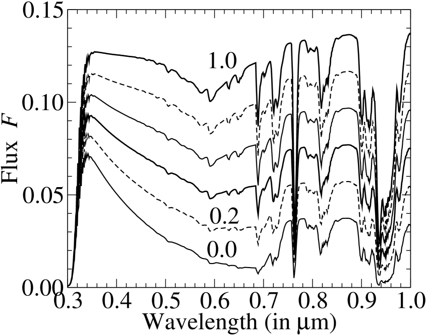
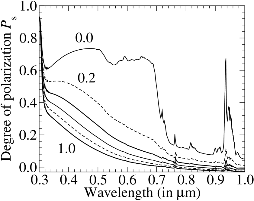
Figure 12: Similar to Fig. 8, except for quasi horizontally inhomogeneous planets with 70$\%$ of their surfaces covered by specular reflecting ocean and 30$\%$ by deciduous forest. The cloud coverage ranges from 0.0 to 1.0, in steps of 0.2. The planetary phase angle, $\alpha$, is 90^∘.

Figure 12 shows the flux and degree of polarization of light reflected by an exoplanet that has, like the Earth, 70 $\%$ of its surface covered by a specular reflecting ocean and 30 $\%$ by deciduous forest. The cloud coverage ranges from 0.0 (a clear atmosphere) to 1.0 (a completely overcast sky) in steps of 0.2. Recall that the mean global cloud coverage of the Earth is about 0.67 (Rossow et al. 1996). Note that to simulate $F$ and $P_{\rm s}$ of the cloudy fractions of the planets, we combined the cloudy, ocean–covered planets with the cloudy, forest–covered planets. In Eq. 15, we thus used $N=4$.

The main, not surprising difference between the flux of the clear, quasi horizontally inhomogeneous planet from Fig. 12a, and that of the clear, horizontally homogeneous forest–covered planet in Fig. 8a, is that the red edge (for $\lambda>0.7~{}\mu$m) that is characteristic for reflection by vegetation, is much less strong when 70 $\%$ of the planet is covered by ocean than when the whole planet is covered by vegetation (the red edge continuum is approximately 0.035 for the inhomogeneous planet and 0.11 for the homogeneous one). The (black) ocean all but removes the local maximum in $F$ at green wavelengths (between 0.5 and 0.6 $\mu$m) which is due to chlorophyll in the vegetation. In $P_{\rm s}$ (Fig. 12b), the ocean somewhat changes the spectral shape of the red edge feature, and decreases its depth by about 0.04 (at $\lambda=0.87~{}\mu$m) when compared to Fig. 8b. The ocean signficantly changes the spectral feature in $P_{\rm s}$ that is due to chlorofyll: for the clear, completely forest–covered planet (Fig. 8b), the minimum $P_{\rm s}$ across this feature is 0.38 while it is 0.63 for the clear planet in Fig. 12b. Finally, in $P_{\rm s}$, the gaseous absorption bands are stronger for the clear planet covered by ocean and forest, than for the clear, forest–covered planet.

From Fig. 12a, it is clear that $F$ in the continuum is very sensitive to the cloud coverage. The continuum $P_{\rm s}$ is also sensitive to the cloud coverage, but this sensitivity decreases with increasing cloud coverage, in particularly at the longer wavelengths.

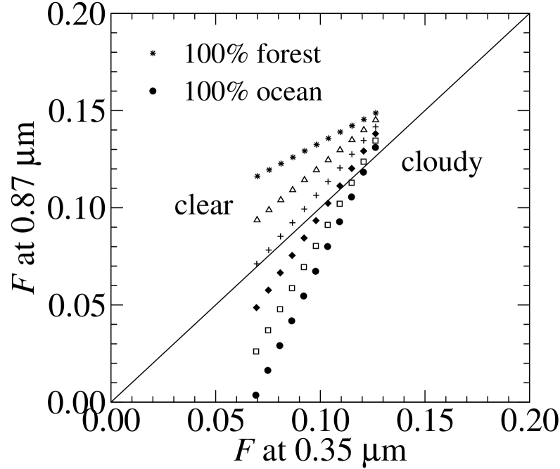
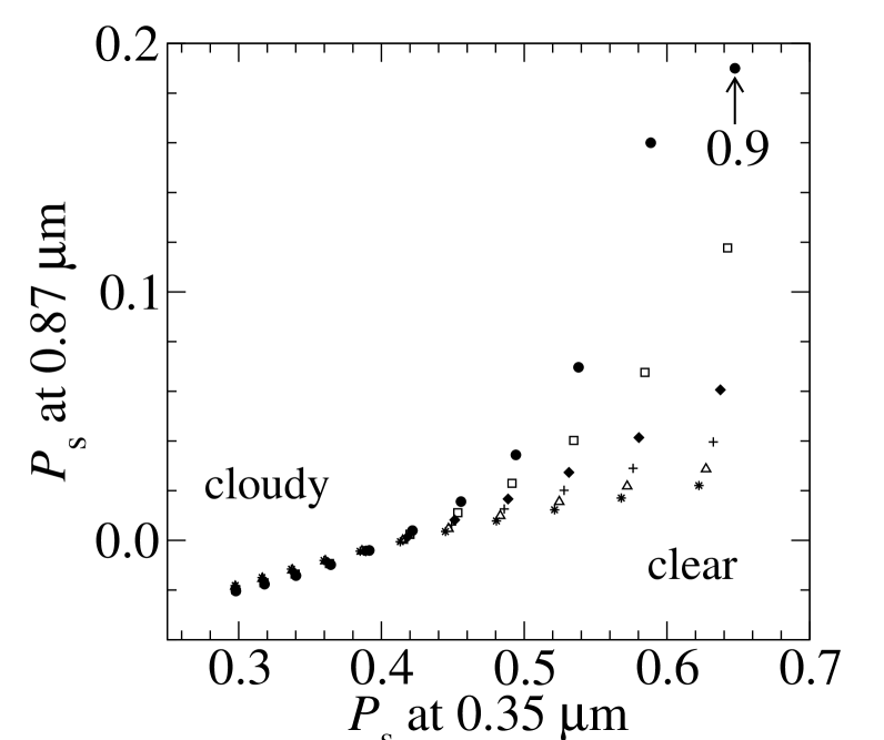
Figure 13: The relations between $F$ (left) and $P_{\rm s}$ (right) in the blue ($\lambda=0.35~{}\mu$m) and the near–infrared ($\lambda=0.87~{}\mu$m) for planets with ratios between ocean and forest–surface coverage ranging from 0.0 (100 $\%$ covered by forest, indicated by the stars), to 0.0 (100 $\%$ covered by ocean, indicated by the black circles), with steps of 0.2. In addition, the cloud coverage ranges from 0.0 to 1.0, in steps of 0.1. The planetary phase angle, $\alpha$, is 90^∘. Note that we have included the line $F$(0.87 $\mu$m)=$F$(0.35 $\mu$m) in the graph on the left, and that at $\lambda=0.87~{}\mu$m, $P_{\rm s}$ of the clear, 100 $\%$ ocean planet falls of the vertical figure scale; its value is 0.9.

To get more insight into the sensitivity of the shape of the flux and polarization spectra to the surface and the cloud coverage, we have plotted in Fig. 13, $F$ and $P_{\rm s}$ in the near–infrared continuum ($\lambda=0.87~{}\mu$m) against $F$ and $P_{\rm s}$ in the blue continuum ($\lambda=0.35~{}\mu$m) for planets with surface coverage ratios ranging from 0.0 (100 $\%$ forest) to 1.0 (100 $\%$ ocean), in steps of 0.2. The cloud coverage ranges from 0.0 (a clear planet) to 1.0 (a completely cloudy planet). Looking at the reflected fluxes (Fig. 13a), it can be seen that for a given cloud coverage, $F$ in the blue is virtually independent of the surface coverage (ocean or forest), while in the near–infrared, the sensitivity of $F$ to the surface coverage depends strongly on the cloud coverage: it is relatively large when the cloud coverage is small, and relatively small when the cloud coverage is large, as could be expected. Fig. 13a shows that our completely cloudy planets are somewhat brighter in the near–infrared than in the blue (assuming a wavelength independent stellar flux, or, after correcting observations for the incoming stellar flux). Looking at the degree of polarization of the reflected fluxes (Fig. 13b), it is clear that the larger the cloud coverage, the smaller the dependence of $P_{\rm s}$ at both 0.35 $\mu$m and 0.87 $\mu$m on the surface coverage. For a given cloud coverage smaller than about 0.5, $P_{\rm s}$ can be seen to depend on the surface coverage. In particular, the larger the fraction of ocean on the planet, the larger $P_{\rm s}$ in the near–infrared. In the blue, $P_{\rm s}$ also increases with increasing fraction of ocean coverage, but only slightly so.

It is important to remember that the precise location of the data points in Fig. 13, and thus the retrieval opportunities, will depend on the physical parameters of the model cloud, such as the cloud optical thickness, the microphysical properties of the cloud particles, and the altitude of the cloud. We will explore such dependencies in later studies.

4.3.2 Phase angle dependence and diurnal variation

As a horizontally inhomogeneous planet like the Earth rotates around its axis, the surface fraction of, for example, ocean that is turned towards a distant observer will vary during the day (except when the observer is located precisely above one of the planet’s geographic poles). Assuming a planet with a surface that is covered only by land and water, the diurnal variation of the distribution of land and water across the part of the planetary disk that is illuminated and turned towards a distant observer depends on many factors, such as the actual distribution of land and water across the planet, the sub-observer latitude, the planet’s phase angle, and the location of the terminator (the division between day and night on the planet, that will depend on the obliquity of the planet and the time of year). The variation that can actually be observed, would, of course, also depend on the cloud cover. Calculated diurnal variations of fluxes of Earth-like exoplanets have been presented by Ford et al. (2001), using a single scattering Monte Carlo radiative transfer code and horizontally inhomogeneous model planets, and by Tinetti et al. (2006b).

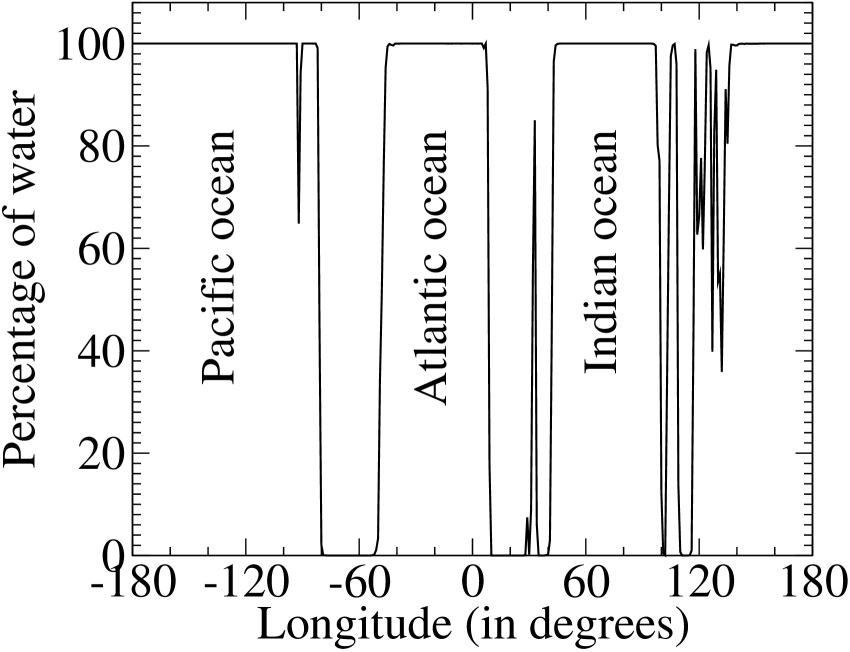
Figure 14: The percentage of surface covered by water along the equator of the Earth. This curve is derived from data of the Clouds and the Earth’s Radiant Energy System (CERES) instrument on NASA’s Earth Observing System (EOS). The longitude of 0^∘ corresponds to the meridian of Greenwich.

Here, we will show a few examples of the diurnal variation of the flux and in particular the degree of polarization of a quasi horizontally inhomogeneous exoplanet with a longitudinal distribution of land and water similar to that along the Earth’s equator (see Fig. 14). For simplicity, we assume the distribution is latitude independent (we thus have a planet with ”vertical stripes”). Furthermore, the distant observer is located in the planet’s equatorial plane, and we assume the planet’s obliquity equals zero. Our model planets are somewhat simpler than those of Ford et al. (2001) and Tinetti et al. (2006b), who use realistically horizontally inhomogeneous planets, but we do use multiple scattering, like Tinetti et al. (2006b), and polarization.

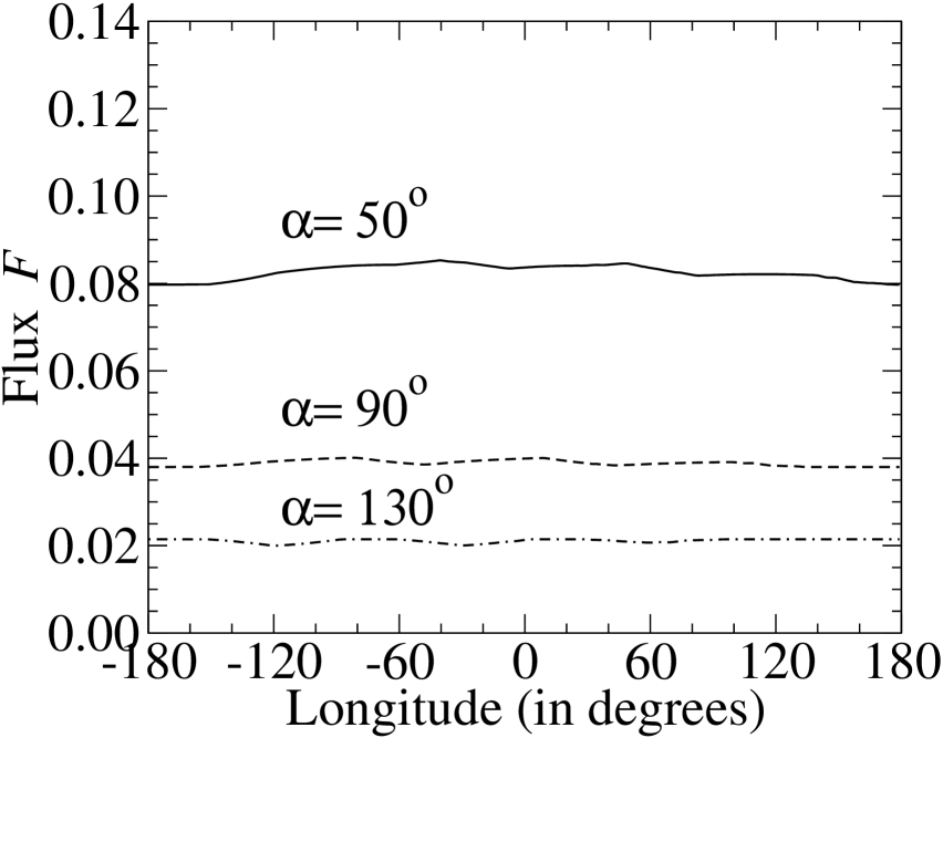
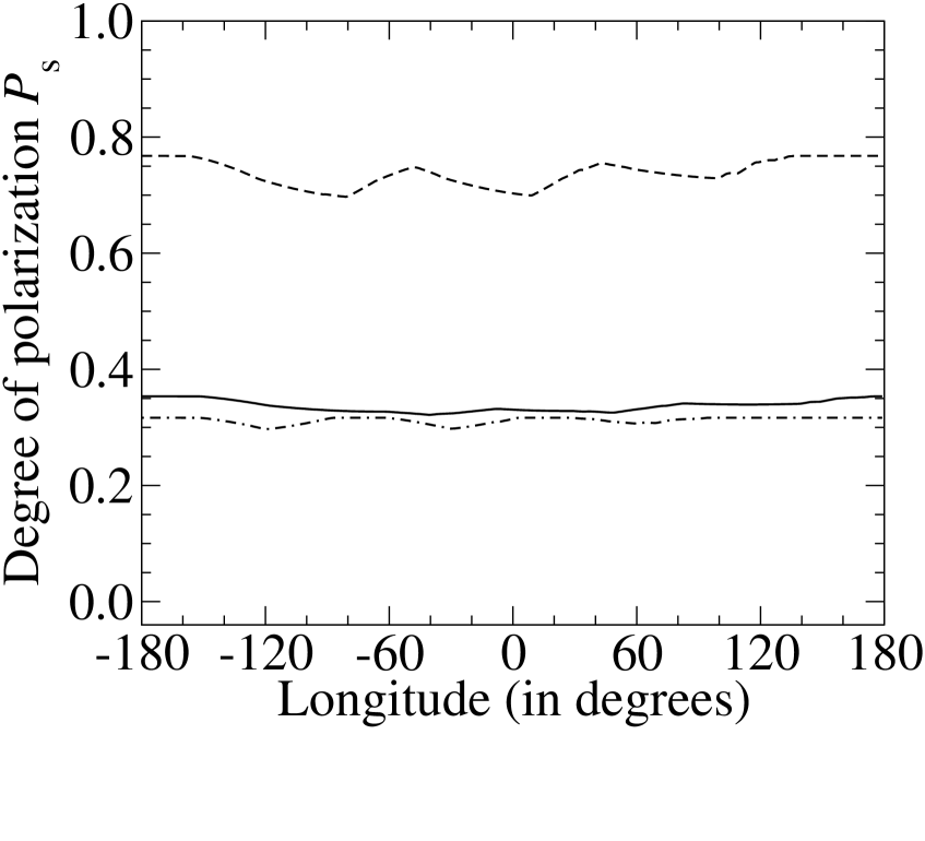
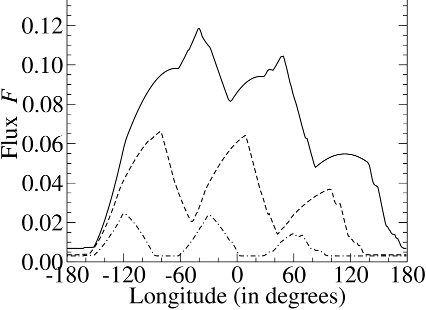
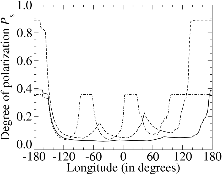
Figure 15: The flux $F$ (left) and degree of polarization $P_{\rm s}$ (right) of starlight reflected by a cloudless quasi horizontally inhomogeneous planet as functions of the sub-observer longitude. The longitudinal distribution of land (covered by vegetation) and water (ocean) is as given in Fig. 14. The planetary phase angles are 50^∘ (solid lines), 90^∘ (dashed lines) and 130^∘ (dash-dotted lines). The upper two panels are for $\lambda=0.44~{}\mu$m, and the lower two panels for $\lambda=0.87~{}\mu$m.

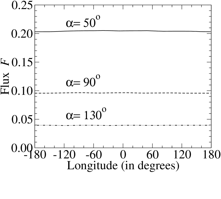
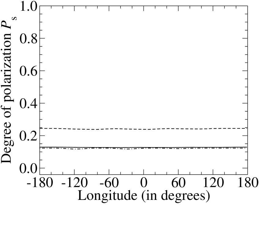
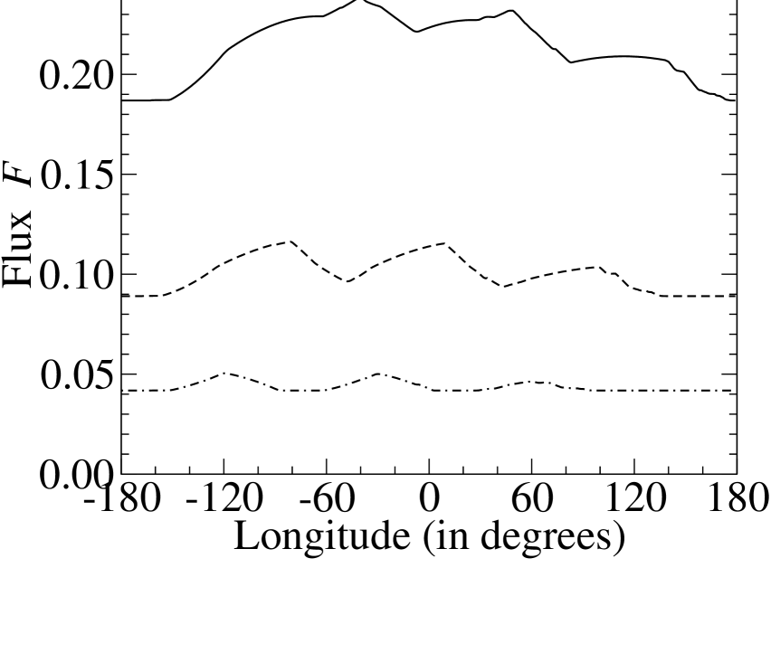
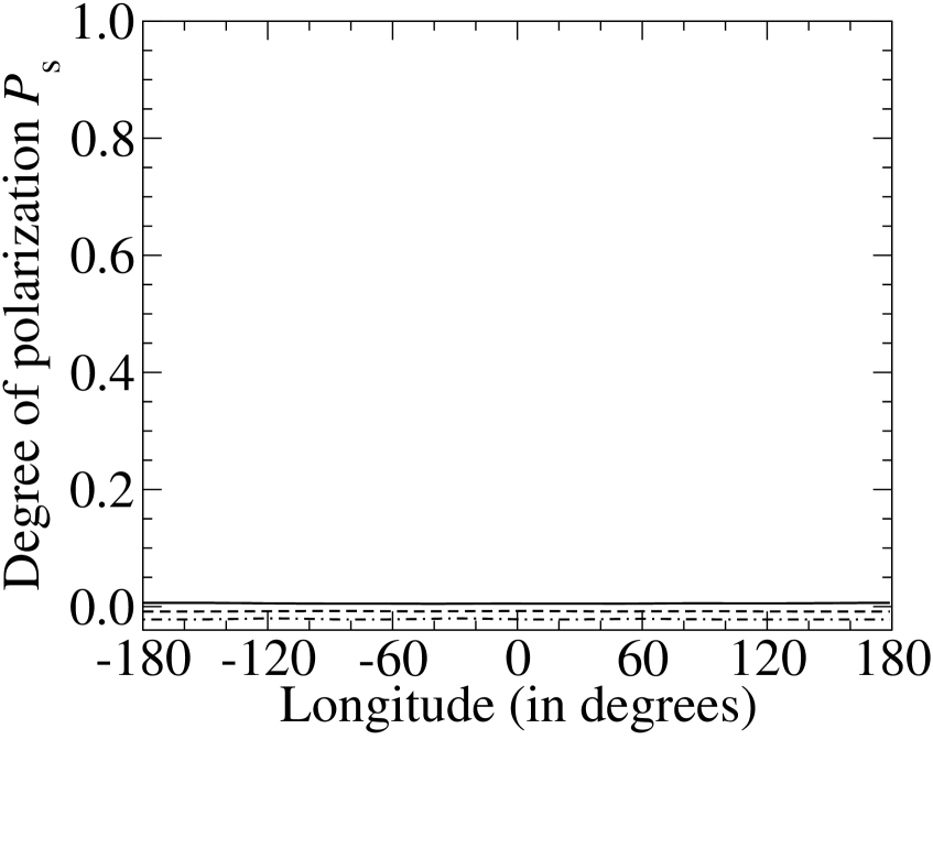
Figure 16: Similar to Fig. 15, except for planets with a cloud coverage of 0.67 (Rossow et al. 1996). The planetary phase angles are 50^∘ (solid lines), 90^∘ (dashed lines) and 130^∘ (dash-dotted lines). The upper two panels are for $\lambda=0.44~{}\mu$m, and the lower two panels for $\lambda=0.87~{}\mu$m.

In Fig. 15, we have plotted $F$ and $P_{\rm s}$ of a cloudless planet seen under phase angles of 50^∘ (when more than half of the illuminated part of the planetary disk is visible), 90^∘ (quadrature, when half of the illuminated planetary disk is visible) and 130^∘ (when less than half of the illuminated planetary disk is visible). We show curves for $\lambda=0.44~{}\mu$m, and for $\lambda=0.87~{}\mu$m. Figure 16 is similar to Fig. 15, except that here, like on an average Earth (Rossow et al. 1996), two-thirds of the planet is covered by clouds.

For the cloudless planet (Fig. 15), $F$ and $P_{\rm s}$ show for all three phase angles much more variation in the near-infrared (0.87 $\mu$m) than in the blue (0.44 $\mu$m). This is not surprising, since in the blue, the vegetation and the ocean are both dark, and $F$ and $P_{\rm s}$ are thus mostly determined by the gaseous atmosphere. In the near-infrared, the contrast between the (red edge of the) vegetation and the ocean shows up clearly in both $F$ and $P_{\rm s}$. A similar wavelength dependence of the variation of the reflected flux (at $\alpha=90^{\circ}$) was found by Ford et al. (2001) and by Tinetti et al. (2006b) (the latter have 0.50 to 0.55 $\mu$m as the shortest wavelength region). In the blue (0.44 $\mu$m in our plots, and 0.45 $\mu$m in the plots by Ford et al. (2001)), our reflected flux (for $\alpha=90^{\circ}$) shows far less diurnal variation than that of Ford et al. (2001). This is most likely due to the multiple scattering that we include in our calculations. In the infrared (0.87 $\mu$m in our plots, and 0.75 $\mu$m in the plots by Ford et al. (2001)), our maximum fluxes (for $\alpha=90^{\circ}$) are larger than those of Ford et al. (2001), namely about $0.06$ versus about $0.03$, which cannot be attributed to multiple scattering, because the atmospheric molecular scattering optical thickness at these wavelengths is very small. This difference in maximum flux is most probably due to the difference in surface coverage (vegetation versus Sahara sand and ocean) and hence in surface albedo at these wavelengths.

The diurnal variation in the degree of polarization, $P_{\rm s}$, has not been studied before. In the blue, $P_{\rm s}$ is strongly determined by Rayleigh scattering, and thus depends strongly on the planetary phase angle. Here, the average $P_{\rm s}$ for $\alpha=50^{\circ}$ is very similar to that for $\alpha=130^{\circ}$, because of the symmetry of the degree of polarization of light that is singly scattered by gaseous molecules with the single scattering angle (see Fig. 2b and Fig. 10b). The variation in $P_{\rm s}$ is largest (in absolute sense) for $\alpha=90^{\circ}$, and can be traced back to the difference, at $\alpha=90^{\circ}$, between the curves for the vegetation–covered and the ocean–covered planets in Fig. 10b. Furthermore according to the difference between these two curves in Fig. 10b, the diurnal variation for $\alpha=50^{\circ}$ should be significantly larger than that for $\alpha=130^{\circ}$. However, as can be seen in Fig. 15, the diurnal variation for these two phase angles is similar, and even slightly larger for $\alpha=130^{\circ}$ than for $\alpha=50^{\circ}$. The reason for this is that when $\alpha=130^{\circ}$, the illuminated and observable part of the planet is smaller than for $\alpha=50^{\circ}$, and will therefore have a more uniform surface coverage (either ocean or vegetation) at any given time.

At red wavelengths (lower panels in Fig. 15), where the largest contribution to the reflected light is from the surface, the diurnal variation of the degree of polarization, $P_{\rm s}$, depends strongly on the planetary phase angle; the variation in $P_{\rm s}$ clearly increases with the phase angle.

Next, we discuss the influence of clouds on the diurnal variation of $F$ and $P_{\rm s}$. As can be seen in Fig. 16, and as can be expected from Fig. 10, in the blue (0.44 $\mu$m), our clouds, which cover two-thirds of the planet, smother virtually any diurnal variation in $F$ and in $P_{\rm s}$. In the near-infrared (0.87 $\mu$m), the flux $F$ retains some of the diurnal variation, because at this long wavelength the vegetation has a much higher albedo than the ocean (cf. Fig. 11). The fluxes we calculate for the cloudy planets (and $\alpha=90^{\circ}$) are very similar to those calculated by Ford et al. (2001), because to describe the light reflected by the cloudy regions on their model planets, Ford et al. (2001) apparently do not rely on the single scattering approach they use for the cloud-free planets. Instead they adopt the reflected fluxes presented by Hovenier & Hage (1989) for cloudy planet models, the calculation of which does fully include multiple scattering (though no vegetated surfaces underneath the clouds). Qualitatively, our variation in $F$ is very similar to that shown by Tinetti et al. (2006b), although the normalization is different.

The degree of polarization in the near-infrared shows no measurable variation; the higher albedo of the vegetation only adds more unpolarized light to the total reflected light. All clouds on our model planet are optically thick ($b^{\rm c}=10$ at 0.55 $\mu$m, see Sect. 3). Optically thinner clouds, that depolarize the light less, would probably leave more diurnal variation in $P_{\rm s}$, as would e.g. polarizing vegetation surfaces (Wolstencroft et al. 2007).

With our method for calculating the light reflected by horizontally inhomogeneous planets (i.e. using Eq. 15), light reflected by e.g. the cloud layer effectively comes from all locations on the illuminated and observed part of the planet, instead of from a limited number of locations spread over the planet, which would be a more realistic cloud deck. We might therefore overestimate the contribution of the cloud layer to the total reflected signal. The difference between the signals of our quasi inhomogeneous planets and those of more realistically inhomogeneous planets require more investigation, also with the view on the retrieval of planetary characteristics. Such an investigation should also address the region-to-region variations in time averaged cloud coverage and cloud optical thickness, that are found on Earth when cloud variations on time scales less than a month (i.e. weather) are removed (for cloud data, see Rossow & Dueñas 2004). Although the actual spatial distribution of cloud properties across an extrasolar planet might not resemble that of the Earth, relations between land and cloud coverage. Regarding flux calculations, examples of region-to-region variations in cloud coverage are given by Ford et al. (2001).

5 Summary and conclusion

We have presented numerical simulations of the flux and state (degree and direction) of polarization of starlight reflected by various types of Earth-like extrasolar planets as functions of the wavelength and as functions of the planetary phase angle. Spectral fluxes of Earth-like extrasolar planets have been presented before (see, e.g. Tinetti et al. 2006a, c; Montañés-Rodríguez et al. 2006; Turnbull et al. 2006, and references therein), the spectral variation of the degree of polarization of such planets not.

Our results clearly show that the light reflected by an Earth-like exoplanet can be highly polarized, with the degree and direction of polarization depending on the physical characteristics of the planetary atmosphere and surface, on the illumination and viewing geometries, and on the wavelength. Polarimetry thus appears to be a useful tool to distinguish the (polarized) stellar light that has been reflected by an Earth-like extrasolar planet from the (unpolarized) direct stellar light, and hence to detect Earth-like extrasolar planets.

Our results also show that for given physical properties of the Earth-like extrasolar planet, the degree of polarization of the reflected light has similar spectral features as the flux of this light: there are features related to the surface albedo of the planet and high spectral resolution features that are due to absorption of light by atmospheric gases. The latter features, although due to different gases, were also present in calculated polarization spectra of starlight reflected by extrasolar gaseous planets (Stam et al. 2004). For Earth-like extrasolar planets, the occurence of spectral features due to gaseous absorption in polarization spectra is especially interesting because these features are conserved upon transmission of the light through the Earth’s atmosphere even if it has a similar composition as the extrasolar planet’s atmosphere (although the number of available photons in the absorption bands will be greatly reduced upon traveling through the Earth’s atmosphere if it contains the same absorbing gases as the extrasolar planet’s atmosphere).

Interestingly, the degree of polarization of reflected light appears to have a different sensitivity to the structure and composition of the planetary atmosphere and the albedo of the underlying surface than the flux of the reflected light has. Compared to using only spectroscopy, polarimetry could thus provide additional and different information on the structure and composition of an extrasolar planet’s atmosphere and surface. In particular, we have shown that the degree of polarization at continuum wavelengths around the O₂ $A$-band (around 0.76 nm) is sensitive to the cloud top altitude, whereas the continuum flux in this wavelength region is virtually insensitive to the cloud top altitude. The degree of polarization could thus be used for cloud top altitude determination, a method that is also applied to e.g. observations of the Earth observing POLDER instrument (Deschamps et al. 1994) and its successors. We have also shown that the depth of the O₂ $A$-band in a polarization spectrum is sensitive to the oxygen mixing ratio, whereas the flux in the O₂ $A$-band is sensitive to both the cloud top altitude and the oxygen mixing ratio. Polarimetry could thus help to disentangle crucial information on gaseous mixing ratios and clouds from the sparse, spatially unresolved data that will be available for exoplanets.

Because of the strengths for detecting and characterizing Earth-like exoplanets, as mentioned above, polarimetry is a technique used in SEE-COAST (the Super Earths Explorer – Coronographic Off-Axis Telescope), a space-based telescope for the detection and the characterization of gaseous exoplanets and large rocky exoplanets, so called ’Super-Earths’, (Schneider et al. 2006), that has been proposed to ESA in response to its 2007 Cosmic Vision call.

Our numerical simulations should not only be useful for researchers that are interested in designing and building (spectro)polarimeters for the detection and characterization of Earth-like exoplanets, and for researchers interested in measuring and analyzing the state of polarization of extrasolar planets. Indeed, due to their optics, spectrometers tend to be sensitive to the state of polarization of the incoming light (unless carefully corrected for): the measured fluxes thus depend on the degree and direction of polarization of the observed light (see e.g. Stam et al. 2000b). In case the polarization sensitivity of a spectrometer is known, e.g. because it has been measured during calibration, our numerical simulations can help to estimate the error in the measured flux. To actually correct measured fluxes for the polarization sensitivity of an instrument, one has to know the instrument’s polarization sensitivity and one has to measure the state of polarization of the incoming light, because as our simulations show, this state of polarization varies with the illumination and viewing geometries and with the physical characteristics of the planet. Because the state of polarization is wavelength dependent and shows high spectral resolution features similar to those in the total flux, the state of polarization should be measured with the same spectral resolution as the total flux if one is interested in accurately measuring the depth and shape of e.g. gaseous absorption bands.

Finally, Stam & Hovenier (2005) showed that neglecting polarization when calculating disk–integrated total flux spectra of gaseous planets induces errors of several percent across the continuum and gaseous absorption bands. The reason for these errors is that the flux of scattered light depends on the state of polarization of the incident light (see also Mishchenko et al. 1994; Lacis et al. 1998), and while the incident stellar light can be assumed to be unpolarized (Kemp et al. 1987), it is usually polarized upon the first scattering within the atmosphere. Hence, as long as only single scattering processes are taken into account, polarization does not influence the scattered total flux, and can thus safely be ignored if one is only interested in total fluxes. When multiple scattering has to be accounted for, however, neglecting polarization and treating light as a scalar instead of as a vector, does influence the scattered total flux. The fluxes presented in this paper have all been calculated taking polarization fully into account. To investigate the influence of neglecting polarization on the fluxes of Earth-like extrasolar planets, we performed a number of calculations without polarization.

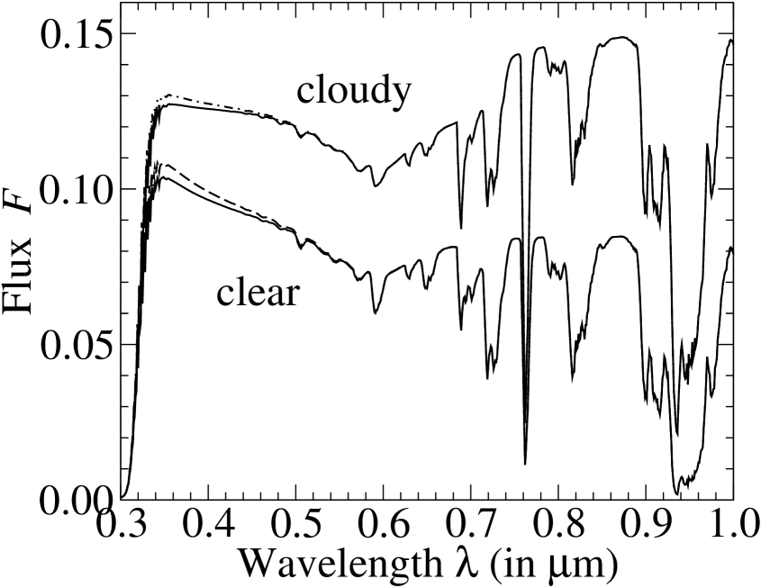
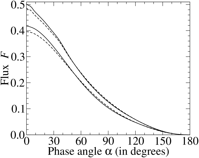
Figure 17: Total reflected fluxes as functions of the wavelength for $\alpha=90^{\circ}$ (left), and as functions of the phase angle for $\lambda=0.35~{}\mu$m (right). The solid lines have been calculated with polarization, and the dashed lines without polarization. The lower two lines are for a homogeneous, cloudfree planet with a surface albedo of 0.4, and the upper two lines are for a homogeneous, cloudy planet with a surface covered by vegetation.

Figure 17 shows total fluxes calculated with and without polarization, for a cloudfree and a cloudy planet, as functions of the wavelength at quadrature, and at $\lambda=0.35~{}\mu$m as functions of the phase angle. For a cloudfree atmosphere with the surface albedo of 0.4, the maximum error is about 4$\%$, at a wavelength of 0.35 $\mu$m. For the cloudy atmosphere with the vegetation underneath, the maximum error is about 2.5 $\%$, also near 0.35 $\mu$m. At other phase angles (Fig. 17b), the relative errors have similar sizes, although they vanish near $\alpha=50^{\circ}$ and 120^∘. The errors have a similar phase angle dependence, but are smaller than those presented for gaseous planets by Stam & Hovenier (2005). The errors are smaller because our Earth-like atmosphere is optically much thinner than that of a gaseous planet, and hence less multiple scattering takes place. That for an Earth-like planet (with a total molecular scattering optical thickness of about 0.1 at $\lambda=0.55~{}\mu$m, see Table 1), the errors will be smaller is also clear from Fig. 5 of Stam & Hovenier (2005), which shows the errors due to neglecting polarization in planetary albedos as functions of the atmospheric molecular scattering optical thickness. The decrease of the error with decreasing molecular scattering optical thickness also explains the decrease of the error with wavelength in Fig. 17, and the smaller error for the cloudy atmosphere. Concluding, for Earth-like model atmospheres, neglecting polarization when calculating fluxes leads to maximum errors of a few percent in the continuum.

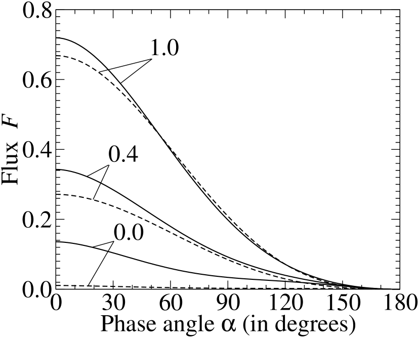
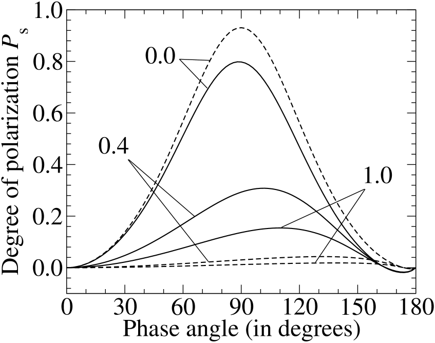
Figure 5: The flux $F$ (left) and the degree of linear polarization $P_{\rm s}$ (right) of starlight reflected by the model planets with $A_{\rm s}=0.0$, 0.4, and 1.0 of Fig. 4 as functions of the phase angle $\alpha$. $F$ and $P_{\rm s}$ have been plotted for two wavelengths: 0.44 $\mu$m (solid lines) and 0.87 $\mu$m (dashed lines).

nr.	$z$	$p$	$T$	O3	H2O	$b^{\rm m}_{\rm sca}$
1	0	1013.00	294	0.3041(-1)	0.1890(+5)	0.203(-1)
2	2	802.00	285	0.3712(-1)	0.9724(+4)	0.167(-1)
3	4	628.00	273	0.4830(-1)	0.3820(+4)	0.136(-1)
4	6	487.00	261	0.6420(-1)	0.1512(+4)	0.111(-1)
5	8	372.00	248	0.9126(-1)	0.6463(+3)	0.876(-2)
6	10	281.00	235	0.1306(0)	0.2475(+3)	0.693(-2)
7	12	209.00	222	0.2216(0)	0.2952(+2)	0.539(-2)
8	14	153.00	216	0.4409(0)	0.6526(+1)	0.404(-2)
9	16	111.00	216	0.7053(0)	0.5727(+1)	0.287(-2)
10	18	81.20	216	0.1295(+1)	0.6161(+1)	0.209(-2)
11	20	59.50	218	0.2171(+1)	0.7655(+1)	0.152(-2)
12	22	43.70	220	0.3162(+1)	0.1193(+2)	0.111(-2)
13	24	32.20	223	0.3852(+1)	0.1924(+2)	0.183(-2)
14	30	13.20	234	0.9131(+1)	0.4379(+2)	0.950(-3)
15	40	3.33	258	0.7431(+1)	0.2077(+2)	0.229(-3)
16	50	9.51(-1)	276	0.2728(+1)	0.1065(+1)	0.915(-4)
17	100	3.00(-4)	210	0.5191(-1)	0.3216(+1)	-

Table 1: The altitude $z$ (in km), the pressure $p$ (in hPa), the temperature $T$ (in K), and the ozone (O₃) and watervapor (H₂O) mixing ratios (in ppm, or parts per million) at the 17 levels of the model atmospheres (McClatchey et al. 1972). Also given is the molecular scattering optical thickness $b^{\rm m}_{\rm sca}$ (at $\lambda=0.55~{}\mu$m) of each of the 16 layers of the model atmospheres. The total molecular scattering optical thickness of the model atmosphere is 0.0975 (at $\lambda=0.55~{}\mu$m). Here, $x(-y)$ stands for $x\cdot 10^{-y}$.

References

- Aben et al. (1997) Aben, I., Helderman, F., Stam, D., & Stammes, P. 1997, in Polarization: Measurement, Analysis, and Remote Sensing. Proceedings SPIE 3121, ed. D. Goldstein & R. Chipman, 446–451
- Aben et al. (1999) Aben, I., Helderman, F., Stam, D. M., & Stammes, P. 1999, Geophys. Res. Lett., 26, 591
- Aben et al. (2001) Aben, I., Stam, D. M., & Helderman, F. 2001, Geophys. Res. Lett., 28, 519
- Arnold et al. (2002) Arnold, L., Gillet, S., Lardière, O., Riaud, P., & Schneider, J. 2002, Astron. & Astrophys., 392, 231
- Bailey (2007) Bailey, J. 2007, Astrobiology, 7, 320
- Bates (1984) Bates, D. R. 1984, Planetary Space Scie., 32, 785
- Beuzit et al. (2006) Beuzit, J.-L., Feldt, M., Dohlen, K., et al. 2006, The Messenger, 125, 29
- Bréon & Henriot (2006) Bréon, F. M. & Henriot, N. 2006, Journal of Geophysical Research (Oceans), 111, 6005
- Chowdhary et al. (2002) Chowdhary, J., Cairns, B., & Travis, L. D. 2002, Journal of Atmospheric Sciences, 59, 383
- Cox & Munk (1954) Cox, C. & Munk, W. 1954, Journal of the Optical Society of America (1917-1983), 44, 838
- de Haan et al. (1987) de Haan, J. F., Bosma, P. B., & Hovenier, J. W. 1987, Astron. & Astrophys., 183, 371
- de Rooij & van der Stap (1984) de Rooij, W. A. & van der Stap, C. C. A. H. 1984, Astron. & Astrophys., 131, 237
- Deschamps et al. (1994) Deschamps, P. Y., Bréon, F. M., Leroy, M., et al. 1994, IEEE Trans. Geosci. Remote Sens., 32, 598
- Fischer et al. (1991) Fischer, J., Cordes, W., Schmitz-Peiffer, A., Renger, W., & Mörl, P. 1991, Journal of Applied Meteorology, 30, 1260
- Fischer & Grassl (1991) Fischer, J. & Grassl, H. 1991, Journal of Applied Meteorology, 30, 1245
- Ford et al. (2001) Ford, E. B., Seager, S., & Turner, E. L. 2001, Nature, 412, 885
- Gandorfer et al. (2004) Gandorfer, A. M., Steiner, H. P. P. P., Aebersold, F., et al. 2004, Astron. & Astrophys., 422, 703
- Gisler et al. (2004) Gisler, D., Schmid, H. M., Thalmann, C., et al. 2004, in Presented at the Society of Photo-Optical Instrumentation Engineers (SPIE) Conference, Vol. 5492, Ground-based Instrumentation for Astronomy. Edited by Alan F. M. Moorwood and Iye Masanori. Proceedings of the SPIE, Volume 5492, pp. 463-474 (2004)., ed. A. F. M. Moorwood & M. Iye, 463–474
- Grainger & Ring (1962) Grainger, J. F. & Ring, J. 1962, Nature, 193, 762
- Haferman et al. (1997) Haferman, J. L., Smith, T. F., & Krajewski, W. F. 1997, Journal of Quantitative Spectroscopy and Radiative Transfer, 58, 379
- Hamdani et al. (2006) Hamdani, S., Arnold, L., Foellmi, C., et al. 2006, Astron. & Astrophys., 460, 617
- Hansen & Hovenier (1974a) Hansen, J. E. & Hovenier, J. W. 1974a, Journal of Atmospheric Sciences, 31, 1137
- Hansen & Hovenier (1974b) Hansen, J. E. & Hovenier, J. W. 1974b, in IAU Symp. 65: Exploration of the Planetary System, 197–200
- Hansen & Travis (1974) Hansen, J. E. & Travis, L. D. 1974, Space Science Reviews, 16, 527
- Hough & Lucas (2003) Hough, J. H. & Lucas, P. W. 2003, in ESA SP-539: Earths: DARWIN/TPF and the Search for Extrasolar Terrestrial Planets, 11–17
- Hough et al. (2006a) Hough, J. H., Lucas, P. W., Bailey, J. A., Tamura, M., & Hirst, E. 2006a, in the Society of Photo-Optical Instrumentation Engineers (SPIE) Conference, Vol. 6269, Ground-based and Airborne Instrumentation for Astronomy. Edited by McLean, Ian S.; Iye, Masanori. Proceedings of the SPIE, Volume 6269, pp. 62690S (2006).
- Hough et al. (2006b) Hough, J. H., Lucas, P. W., Bailey, J. A., et al. 2006b, Pub. Astron. Soc. Pac., 118, 1305
- Hovenier & Hage (1989) Hovenier, J. W. & Hage, J. I. 1989, Astron. & Astrophys., 214, 391
- Hovenier et al. (2004) Hovenier, J. W., van der Mee, C., & Domke, H. 2004, Transfer of Polarized Light in Planetary Atmospheres; Basic Concepts and Practical Methods (Kluwer, Dordrecht; Springer, Berlin)
- Joos & Schmid (2007) Joos, F. & Schmid, H. M. 2007, Astron. & Astrophys., 463, 1201
- Joos et al. (2005) Joos, F., Schmid, H. M., Gisler, D., et al. 2005, in Astronomical Society of the Pacific Conference Series, ed. A. Adamson, C. Aspin, & C. Davis, 189–+
- Keller (2006) Keller, C. U. 2006, in Presented at the Society of Photo-Optical Instrumentation Engineers (SPIE) Conference, Vol. 6269, Ground-based and Airborne Instrumentation for Astronomy. Edited by McLean, Ian S.; Iye, Masanori. Proceedings of the SPIE, Volume 6269, pp. 62690T (2006).
- Kemp et al. (1987) Kemp, J. C., Henson, G. D., Steiner, C. T., & Powell, E. R. 1987, Nature, 326, 270
- Kiang et al. (2007) Kiang, N. Y., Segura, A., Tinetti, G., et al. 2007, Astrobiology, 7, 252
- Koepke (1984) Koepke, P. 1984, Appl. Optics, 23, 1816
- Kuze & Chance (1994) Kuze, A. & Chance, K. V. 1994, J. Geophys. Res., 99, 14481
- Lacis et al. (1998) Lacis, A. A., Chowdhary, J., Mishchenko, M. I., & Cairns, B. 1998, Geophys. Res. Lett., 25, 135
- Lacis & Oinas (1991) Lacis, A. A. & Oinas, V. 1991, J. Geophys. Res., 96, 9027
- Liou & Takano (2002) Liou, K. N. & Takano, Y. 2002, Geophys. Res. Lett., 29, 27
- McClatchey et al. (1972) McClatchey, R., Fenn, R., Selby, J., Volz, F., & Garing, J. 1972, Optical Properties of the Atmosphere, AFCRL-72.0497 (U.S. Air Force Cambridge Research Labs)
- Mishchenko et al. (1994) Mishchenko, M. I., Lacis, A. A., & Travis, L. D. 1994, Journal of Quantitative Spectroscopy and Radiative Transfer, 51, 491
- Montañés-Rodríguez et al. (2006) Montañés-Rodríguez, P., Pallé, E., Goode, P. R., & Martín-Torres, F. J. 2006, Astrophys. J., 651, 544
- Peck & Reeder (1972) Peck, E. R. & Reeder, K. 1972, Journal of the Optical Society of America (1917-1983), 62, 958
- Preusker et al. (1995) Preusker, R., Böttger, U., & Fischer, J. 1995, in Atmospheric Sensing and Modeling II. Proceedings SPIE 2582, ed. R. Santer, 13–20
- Rossow & Dueñas (2004) Rossow, W. B. & Dueñas, E. N. 2004, Bulletin of the American Meteorological Society, vol. 85, Issue 2, pp.167-172, 85, 167
- Rossow et al. (1996) Rossow, W. B., Walker, A. W., Beuschel, D. E., & Roiter, M. D. 1996, International Satellite Cloud Climatology Project (ISCCP) Documentation of New Cloud Datasets. WMO/TD-No. 737 (World Meteorological Organization, Geneva, Switzerland)
- Rothman et al. (2005) Rothman, L. S., Jacquemart, D., Barbe, A., et al. 2005, Journal of Quantitative Spectroscopy and Radiative Transfer, 96, 139
- Saar & Seager (2003) Saar, S. H. & Seager, S. 2003, in Astronomical Society of the Pacific Conference Series, 529–534
- Sagan et al. (1993) Sagan, C., Thompson, W. R., Carlson, R., Gurnett, D., & Hord, C. 1993, Nature, 365, 715
- Saiedy et al. (1967) Saiedy, F., Jacobowitz, H., & Wark, D. Q. 1967, Journal of Atmospheric Sciences, 24, 63
- Schmid et al. (2005) Schmid, H. M., Gisler, D., Joos, F., et al. 2005, in Astronomical Society of the Pacific Conference Series, Vol. 343, Astronomical Polarimetry: Current Status and Future Directions, ed. A. Adamson, C. Aspin, C. Davis, & T. Fujiyoshi, 89–+
- Schmid et al. (2006) Schmid, H. M., Joos, F., & Tschan, D. 2006, Astron. & Astrophys., 452, 657
- Schneider et al. (2006) Schneider, J., Riaud, P., Tinetti, G., et al. 2006, in SF2A-2006: Semaine de l’Astrophysique Francaise, ed. D. Barret, F. Casoli, G. Lagache, A. Lecavelier, & L. Pagani, 429–+
- Seager et al. (2005) Seager, S., Turner, E. L., Schafer, J., & Ford, E. B. 2005, Astrobiology, 5, 372
- Seager et al. (2000) Seager, S., Whitney, B. A., & Sasselov, D. D. 2000, Astrophys. J., 540, 504
- Segura et al. (2005) Segura, A., Kasting, J. F., Meadows, V., et al. 2005, Astrobiology, 5, 706
- Sengupta & Maiti (2006) Sengupta, S. & Maiti, M. 2006, Astrophys. J., 639, 1147
- Shkuratov et al. (2005) Shkuratov, Y., Kreslavsky, M., Kaydash, V., et al. 2005, Icarus, 176, 1
- Sromovsky (2005) Sromovsky, L. A. 2005, Icarus, 173, 254
- Stam et al. (2000a) Stam, D., de Haan, J., Hovenier, J., & Stammes, P. 2000a, Journal of Quantitative Spectroscopy and Radiative Transfer, 64, 131
- Stam et al. (2005) Stam, D., Hovenier, J., & Waters, L. 2005, in Astronomical Society of the Pacific Conference Series, ed. A. Adamson, C. Aspin, & C. Davis, 207–+
- Stam (2003) Stam, D. M. 2003, in ESA SP-539: Earths: DARWIN/TPF and the Search for Extrasolar Terrestrial Planets, 615–619
- Stam et al. (2002) Stam, D. M., Aben, I., & Helderman, F. 2002, Journal of Geophysical Research (Atmospheres), AAC 1
- Stam et al. (2000b) Stam, D. M., De Haan, J. F., Hovenier, J. W., & Aben, I. 2000b, J. Geophys. Res., 22379
- Stam et al. (1999) Stam, D. M., De Haan, J. F., Hovenier, J. W., & Stammes, P. 1999, J. Geophys. Res., 104, 16843
- Stam et al. (2006) Stam, D. M., de Rooij, W. A., Cornet, G., & Hovenier, J. W. 2006, Astron. & Astrophys., 452, 669
- Stam et al. (2003) Stam, D. M., Hovenier, J., & Waters, R. 2003, in Astronomical Society of the Pacific Conference Series, Vol. 294, Scientific Frontiers in Research on Extrasolar Planets, ed. D. Deming & S. Seager, 535–538
- Stam & Hovenier (2005) Stam, D. M. & Hovenier, J. W. 2005, Astron. & Astrophys., 444, 275
- Stam et al. (2004) Stam, D. M., Hovenier, J. W., & Waters, L. B. F. M. 2004, Astron. & Astrophys., 428, 663
- Stammes et al. (1994) Stammes, P., Kuik, F., & de Haan, J. 1994, in Proceedings PIERS 1994, Kluwer Acad., Dordrecht, ed. B. e. a. Arbesser-Rastburg, 2255–2259
- Tinetti et al. (2006a) Tinetti, G., Meadows, V. S., Crisp, D., et al. 2006a, Astrobiology, 6, 34
- Tinetti et al. (2006b) Tinetti, G., Meadows, V. S., Crisp, D., et al. 2006b, Astrobiology, 6, 881
- Tinetti et al. (2006c) Tinetti, G., Rashby, S., & Yung, Y. L. 2006c, Astrophys. J., 644, L129
- Turnbull et al. (2006) Turnbull, M. C., Traub, W. A., Jucks, K. W., et al. 2006, Astrophys. J., 644, 551
- van de Hulst (1957) van de Hulst, H. C. 1957, Light Scattering by Small Particles (J. Wiley and Sons, New York.)
- van de Hulst (1980) van de Hulst, H. C. 1980, Multiple Light Scattering, Tables, Formulas, and Applications, Vols. 1 and 2 (Academic Press, New York.)
- van Deelen et al. (2005) van Deelen, R., Landgraf, J., & Aben, I. 2005, Journal of Quantitative Spectroscopy and Radiative Transfer, 95, 309
- Wolstencroft et al. (2007) Wolstencroft, R. D., Breon, F., & Tranter, G. 2007, in American Astronomical Society Meeting Abstracts, Vol. 210, American Astronomical Society Meeting Abstracts, 09.06–+
- Wolstencroft & Raven (2002) Wolstencroft, R. D. & Raven, J. A. 2002, Icarus, 157, 535
- Woolf et al. (2002) Woolf, N. J., Smith, P. S., Traub, W. A., & Jucks, K. W. 2002, Astrophys. J., 574, 430