Abstract

In this article, we calculate the strong coupling constant $g_{\Delta N\pi}$ and study the strong decay $\Delta^{++}\to p\pi$ with the light-cone QCD sum rules. The numerical value of the strong coupling constant $g_{\Delta N\pi}$ is consistent with the experimental data. The small discrepancy maybe due to failure to take into account the perturbative $\mathcal{O}(\alpha_{s})$ corrections.

PACS numbers: 13.30.-a; 13.75.Gx

1 Introduction

The $\Delta(1232)$ resonance dominates many nuclear phenomena at energies above the pion-production threshold and plays an important role in the physics of the strong interaction. It is almost an ideal elastic $\pi N$ resonance, and decays into the nucleon and pion ($\Delta\to N\pi$) with the branching fraction about $99\%$. The only other (electromagnetic) decay channel ($\Delta\to N\gamma$) contributes less than $1\%$ to the total decay width [1]. There is a very small mass gap (less than $300\rm{MeV}$) between the $\Delta$ and the nucleon, and the $\Delta(1232)$ is taken as an explicit dynamical degree of freedom in the heavy baryon chiral perturbation theory [2].

In this article, we calculate the strong coupling constant $g_{\Delta N\pi}$ with the light-cone QCD sum rules, and study the decay width $\Gamma_{\Delta\to N\pi}$. The strong coupling constants of the octet baryons with the vector and pseudoscalar mesons $g_{NNV}$ and $g_{NNP}$ have been calculated with the light-cone QCD sum rules [3]. The light-cone QCD sum rules carry out the operator product expansion near the light-cone $x^{2}\approx 0$ instead of the short distance $x\approx 0$ while the nonperturbative hadronic matrix elements are parameterized by the light-cone distribution amplitudes instead of the vacuum condensates [4, 5]. The nonperturbative parameters in the light-cone distribution amplitudes are calculated with the conventional QCD sum rules and the values are universal [6].

The article is arranged as: in Section 2, we derive the strong coupling constant $g_{\Delta N\pi}$ with the light-cone QCD sum rules; in Section 3, the numerical result and discussion; and Section 4 is reserved for conclusion.

2 Strong coupling constant $g_{\Delta N\pi}$ with light-cone QCD sum rules

In the following, we write down the two-point correlation function $\Pi_{\mu}(p,q)$,

$$\Pi_{\mu}(p,q) = i\int d^{4}x\,e^{-iq\cdot x}\,\langle 0|T\left\{J_{p}(0)\bar{J}_{\mu}(x)\right\}|\pi(p)\rangle\,,$$ (1)

$$J_{p}(x) = \epsilon^{abc}u^{T}_{a}(x)C\gamma_{\mu}u_{b}(x)\gamma_{5}\gamma^{\mu}d_{c}(x)\,,$$

$$J_{\mu}(x) = \epsilon^{abc}u^{T}_{a}(x)C\gamma_{\mu}u_{b}(x)u_{c}(x)\,,$$ (2)

where the baryon currents $J_{p}(x)$ and $J_{\mu}(x)$ interpolate the octet baryon $p$ and decuplet baryon $\Delta^{++}$ respectively [7], the external state $\pi$ has the four momentum $p_{\mu}$ with $p^{2}=m_{\pi}^{2}$ . The general form of the proton current can be written as [8]

$$J_{p}(x,t) = \epsilon_{abc}\left\{\left[u_{a}^{T}(x)Cd_{b}(x)\right]\gamma_{5}u_{c}(x)+t\left[u_{a}^{T}(x)C\gamma_{5}d_{b}(x)\right]u_{c}(x)\right\}\,,$$

in the limit $t=-1$, we recover the Ioffe current. If we retain the additional parameter $t$ and choose the ideal value, the sum rule maybe improved, in this article, we choose the Ioffe current for simplicity. The correlation function $\Pi_{\mu}(p,q)$ can be decomposed as

$$\Pi_{\mu}(p,q) = \Pi\sigma_{\alpha\beta}p^{\alpha}q^{\beta}p_{\mu}+\Pi_{A1}p_{\mu}+\Pi_{A2}\not\!\!qp_{\mu}+\Pi_{A3}\not\!\!pp_{\mu}+$$ (3)

$$\Pi_{B1}q_{\mu}+\Pi_{B2}\not\!\!qq_{\mu}+\Pi_{B3}\not\!\!pq_{\mu}+\Pi_{B4}\sigma_{\alpha\beta}p^{\alpha}q^{\beta}q_{\mu}+$$

$$\Pi_{C1}\gamma_{\mu}+\Pi_{C2}\not\!\!q\gamma_{\mu}+\Pi_{C3}\not\!\!p\gamma_{\mu}+\Pi_{C4}\epsilon_{\mu\nu\alpha\beta}\gamma^{\nu}\gamma_{5}p^{\alpha}q^{\beta}$$

due to the Lorentz invariance, where the $\Pi$ and $\Pi_{i}$ are Lorentz invariant functions of $p$ and $q$. In this article, we choose the tensor structure $\sigma_{\alpha\beta}p^{\alpha}q^{\beta}p_{\mu}$ for analysis.

The strong coupling among the $\Delta$, $p$ and $\pi$ can be described by the following chiral Lagrangian [2],

$$\mathcal{L}(x) = g_{\Delta N\pi}\left[\bar{\Delta}^{\mu}(x)\partial_{\mu}\pi(x)N(x)+\bar{N}(x)\partial_{\mu}\pi(x)\Delta^{\mu}(x)\right]\,.$$ (4)

Basing on the quark-hadron duality [6], we can insert a complete series of intermediate states with the same quantum numbers as the current operators $J_{p}(x)$ and $J_{\mu}(x)$ into the correlation function $\Pi_{\mu}(p,q)$ to obtain the hadronic representation. After isolating the ground state contributions from the pole terms of the baryons $p$ and $\Delta$, we get the following result ,

$$\Pi_{\mu}(p,q) = \frac{\langle 0|J_{p}(0)|N(q+p)\rangle\langle N(q+p)|\Delta(q)\pi(p)\rangle\langle\Delta(q)|\bar{J}_{\mu}(0)|0\rangle}{\left\{M_{p}^{2}-(q+p)^{2}\right\}\left\{M_{\Delta}^{2}-q^{2}\right\}}+\cdots$$ (5)

$$= \frac{\lambda_{p}\lambda_{\Delta}}{\left\{M_{p}^{2}-(q+p)^{2}\right\}\left\{M_{\Delta}^{2}-q^{2}\right\}}\left\{\frac{g_{\Delta N\pi}}{3}\sigma_{\alpha\beta}p_{\alpha}q_{\beta}p_{\mu}+\cdots\right\}+\cdots\,,$$

where the following definitions have been used,

$$\langle 0|J_{p}(0)|N(p)\rangle = \lambda_{p}U(p,s)\,,$$

$$\langle 0|J_{\mu}(0)|\Delta(p)\rangle = \lambda_{\Delta}U_{\mu}(p,s)\,,$$

$$\sum_{s}U(p,s)\overline{U}(p,s) = \!\not\!{p}+M_{p}\,,$$

$$\sum_{s}U_{\mu}(p,s)\overline{U}_{\nu}(p,s) = -(\!\not\!{p}+M_{\Delta})\left\{g_{\mu\nu}-\frac{\gamma_{\mu}\gamma_{\nu}}{3}-\frac{2p_{\mu}p_{\nu}}{3M_{\Delta}^{2}}+\frac{p_{\mu}\gamma_{\nu}-p_{\nu}\gamma_{\mu}}{3M_{\Delta}}\right\}\,,$$

$$\langle N(q^{\prime})|\Delta(q)\pi(p)\rangle = ig_{\Delta N\pi}\overline{U}(q^{\prime},s^{\prime})U_{\mu}(q,s)p^{\mu}\,,$$ (6)

the last identity corresponds to the phenomenological Lagrangian in Eq.(4).

The current $J_{\mu}(x)$ couples not only to the isospin $I=\frac{3}{2}$ and spin-parity $J^{P}=\frac{3}{2}^{+}$ states, but also to the isospin $I=\frac{3}{2}$ and spin-parity $J^{P}=\frac{1}{2}^{-}$ states. For a generic $\frac{1}{2}^{-}$ resonance $\Delta^{*}$ [9],

$$\langle 0|J_{\mu}(0)|\Delta^{*}(p)\rangle=\lambda_{*}(\gamma_{\mu}-4\frac{p_{\mu}}{M_{*}})U^{*}(p,s)\,,$$ (7)

where $\lambda^{*}$ is the pole residue and $M_{*}$ is the mass. The spinor $U^{*}(p,s)$ satisfies the usual Dirac equation $(\not\!\!p-M_{*})U^{*}(p)=0$. If we take the phenomenological Lagrangian,

$$\mathcal{L}(x) = g_{\Delta^{*}N\pi}\left\{\bar{\Delta}^{*}(x)N(x)\pi(x)+\bar{N}(x)\Delta^{*}(x)\pi(x)\right\}\,,$$ (8)

which corresponds to $\langle N(q^{\prime})|\Delta^{*}(q)\pi(p)\rangle=g_{\Delta^{*}N\pi}\overline{U}(q^{\prime},s^{\prime})U^{*}(q,s)$, the contributions from the $\frac{1}{2}^{-}$ states can be written as

$$\Pi_{\mu}(p,q) = \frac{g_{\Delta^{*}N\pi}\lambda_{p}\lambda_{*}}{\left\{M_{p}^{2}-(q+p)^{2}\right\}\left\{M_{*}^{2}-q^{2}\right\}}\left\{(\not\!\!p+\not\!\!q+M_{p})(\not\!\!q+M_{*})(\gamma_{\mu}-4\frac{q_{\mu}}{M_{*}})\right\}$$ (9)

$$+\cdots$$

$$= \Pi_{D}\not\!\!qp_{\mu}+\Pi_{E1}q_{\mu}+\Pi_{E2}\not\!\!qq_{\mu}+\Pi_{E3}\not\!\!pq_{\mu}+\Pi_{E4}\sigma_{\alpha\beta}p^{\alpha}q^{\beta}q_{\mu}+$$

$$\Pi_{F1}\gamma_{\mu}+\Pi_{F2}\not\!\!q\gamma_{\mu}+\Pi_{F3}\not\!\!p\gamma_{\mu}+\Pi_{F4}\epsilon_{\mu\nu\alpha\beta}\gamma^{\nu}\gamma_{5}p^{\alpha}q^{\beta}\,,$$

where the $\Pi_{i}$ are Lorentz invariant functions of $p$ and $q$. If we choose the tensor structure $\sigma_{\alpha\beta}p_{\alpha}q_{\beta}p_{\mu}$, the $\Delta^{*}$ has no contaminations.

In the following, we briefly outline the operator product expansion for the correlation function $\Pi_{\mu}(p,q)$ in perturbative QCD theory. The calculations are performed at the large space-like momentum regions $(q+p)^{2}\ll 0$ and $q^{2}\ll 0$, which correspond to the small light-cone distance $x^{2}\approx 0$ required by the validity of the operator product expansion approach. We write down the ”full” propagator of a massive light quark in the presence of the quark and gluon condensates firstly [4, 6],

$$S_{ab}(x) = \frac{i\delta_{ab}\!\not\!{x}}{2\pi^{2}x^{4}}-\frac{\delta_{ab}m_{q}}{4\pi^{2}x^{2}}-\frac{\delta_{ab}}{12}\langle\bar{q}q\rangle+\frac{i\delta_{ab}}{48}m_{q}\langle\bar{q}q\rangle-\frac{\delta_{ab}x^{2}}{192}\langle\bar{q}g_{s}\sigma Gq\rangle$$ (10)

$$+\frac{i\delta_{ab}x^{2}}{1152}m_{q}\langle\bar{q}g_{s}\sigma Gq\rangle\!\not\!{x}$$

$$-\frac{i}{16\pi^{2}x^{2}}\int_{0}^{1}dv\left[(1-v)g_{s}G_{\mu\nu}(vx)\!\not\!{x}\sigma^{\mu\nu}+vg_{s}G_{\mu\nu}(vx)\sigma^{\mu\nu}\!\not\!{x}\right]$$

$$+\cdots\,,$$

then contract the quark fields in the correlation function $\Pi_{\mu}(p,q)$ with the Wick theorem, and obtain the following result,

$$\Pi_{\mu}(p,q) = 2i\epsilon_{abc}\epsilon_{a^{\prime}b^{\prime}c^{\prime}}\int d^{4}xe^{-iq\cdot x}$$ (11)

$$\left\{Tr\left[\gamma_{\alpha}S_{bb^{\prime}}(-x)\gamma_{\mu}CS^{T}_{aa^{\prime}}(-x)C\right]\gamma_{5}\gamma^{\alpha}\langle 0|d_{c}(0)\bar{u}_{c^{\prime}}(x)|\pi(p)\rangle\right.$$

$$\left.-2\gamma_{5}\gamma^{\alpha}\langle 0|d_{c}(0)\bar{u}_{b^{\prime}}(x)|\pi(p)\rangle\gamma_{\mu}CS^{T}_{aa^{\prime}}(-x)C\gamma_{\alpha}S_{bc^{\prime}}(-x)\right\}\,.$$

Perform the following Fierz re-ordering to extract the contributions from the two-particle and three-particle $\pi$-meson light-cone distribution amplitudes respectively,

$$q^{a}_{\alpha}(0)\bar{q}^{b}_{\beta}(x) = -\frac{1}{12}\delta_{ab}\delta_{\alpha\beta}\bar{q}(x)q(0)-\frac{1}{12}\delta_{ab}(\gamma^{\mu})_{\alpha\beta}\bar{q}(x)\gamma_{\mu}q(0)$$ (12)

$$-\frac{1}{24}\delta_{ab}(\sigma^{\mu\nu})_{\alpha\beta}\bar{q}(x)\sigma_{\mu\nu}q(0)$$

$$+\frac{1}{12}\delta_{ab}(\gamma^{\mu}\gamma_{5})_{\alpha\beta}\bar{q}(x)\gamma_{\mu}\gamma_{5}q(0)$$

$$+\frac{1}{12}\delta_{ab}(i\gamma_{5})_{\alpha\beta}\bar{q}(x)i\gamma_{5}q(0)\,,$$

$$q^{a}_{\alpha}(0)\bar{q}^{b}_{\beta}(x)G^{ba}_{\lambda\tau}(vx) = -\frac{1}{4}\delta_{\alpha\beta}\bar{q}(x)G_{\lambda\tau}(vx)q(0)-\frac{1}{4}(\gamma^{\mu})_{\alpha\beta}\bar{q}(x)\gamma_{\mu}G_{\lambda\tau}(vx)q(0)$$ (13)

$$-\frac{1}{8}(\sigma^{\mu\nu})_{\alpha\beta}\bar{q}(x)\sigma_{\mu\nu}G_{\lambda\tau}(vx)q(0)$$

$$+\frac{1}{4}(\gamma^{\mu}\gamma_{5})_{\alpha\beta}\bar{q}(x)\gamma_{\mu}\gamma_{5}G_{\lambda\tau}(vx)q(0)$$

$$+\frac{1}{4}(i\gamma_{5})_{\alpha\beta}\bar{q}(x)i\gamma_{5}G_{\lambda\tau}(vx)q(0)\,,$$

and substitute the hadronic matrix elements (such as the $\langle 0|{\bar{u}}(x)\gamma_{\mu}\gamma_{5}d(0)|\pi(p)\rangle$, $\langle 0|{\bar{u}}(x)g_{s}\sigma_{\mu\nu}\gamma_{5}G_{\alpha\beta}(vx)d(0)|\pi(p)\rangle$, $\langle 0|{\bar{u}}(x)\sigma_{\mu\nu}\gamma_{5}d(0)|\pi(p)\rangle$, etc.) with the corresponding $\pi$-meson light-cone distribution amplitudes, finally we obtain the spectral density at the coordinate space. Once the spectral density in the coordinate space is obtained, we can translate it into the momentum space with the $D=4+2\epsilon$ dimensional Fourier transform,

$$4\Pi = \frac{2f_{\pi}}{3\pi^{2}}\int_{0}^{1}duu\phi_{\pi}(u)\frac{\Gamma(\epsilon)}{(-Q^{2})^{\epsilon}}-\frac{f_{\pi}m_{\pi}^{2}}{2\pi^{2}}\int_{0}^{1}duuA(u)\frac{\Gamma(1)}{(-Q^{2})^{1}}$$ (14)

$$+\frac{f_{\pi}}{9}\langle\frac{\alpha_{s}GG}{\pi}\rangle\int_{0}^{1}duu\phi_{\pi}(u)\frac{\Gamma(2)}{(-Q^{2})^{2}}$$

$$-\frac{f_{\pi}m_{\pi}^{2}}{36}\langle\frac{\alpha_{s}GG}{\pi}\rangle\int_{0}^{1}duuA(u)\frac{\Gamma(3)}{(-Q^{2})^{3}}$$

$$+\frac{f_{3\pi}\langle\bar{q}q\rangle}{2}\int_{0}^{1}dvv\int_{0}^{1}d\alpha_{g}\int_{0}^{1-\alpha_{g}}d\alpha_{u}$$

$$\frac{\Gamma(2)}{(-Q^{2})^{2}}\mid_{u=\alpha_{u}+v\alpha_{g}}\phi_{3\pi}(\alpha_{u},\alpha_{g},1-\alpha_{u}-\alpha_{g})$$

$$+\frac{f_{\pi}m_{\pi}^{2}}{2\pi^{2}}\int_{0}^{1}dv\int_{0}^{1}d\alpha_{g}\int_{0}^{1-\alpha_{g}}d\alpha_{u}u\frac{\Gamma(1)}{(-Q^{2})^{1}}\mid_{u=\alpha_{u}+v\alpha_{g}}$$

$$\left[(1-9v)V_{\perp}-4(1-2v)A_{\parallel}-4(1-v)A_{\perp}\right](\alpha_{u},\alpha_{g},1-\alpha_{u}-\alpha_{g})$$

$$-\frac{4f_{\pi}m_{\pi}^{2}}{\pi^{2}}\int_{0}^{1}dv\int^{1}_{0}d\alpha_{g}\int_{0}^{1-\alpha_{g}}d\alpha_{u}\int_{0}^{\alpha_{u}}d\alpha\frac{\Gamma(1)}{(-Q^{2})^{1}}\mid_{u=\alpha_{u}+v\alpha_{g}}$$

$$\left[V_{\parallel}+V_{\perp}+(1-2v)(A_{\parallel}+A_{\perp})\right](\alpha,\alpha_{g},1-\alpha-\alpha_{g})$$

$$+\frac{4f_{\pi}m_{\pi}^{2}}{\pi^{2}}\int_{0}^{1}dv(1-v)\int^{1}_{0}d\alpha_{g}\int_{0}^{\alpha_{g}}d\beta\int_{0}^{\beta}d\alpha\frac{\Gamma(1)}{(-Q^{2})^{1}}\mid_{u=1-(1-v)\alpha_{g}}$$

$$\left[V_{\parallel}+V_{\perp}+(1-2v)(A_{\parallel}+A_{\perp})\right](\alpha,\beta,1-\alpha-\beta)\,,$$

where $Q_{\mu}=q_{\mu}+up_{\mu}$ and $Q^{2}=(1-u)q^{2}+u(p+q)^{2}-u(1-u)m_{\pi}^{2}$. The $\epsilon$ is a small positive quantity, after taking the double Borel transform, we can take the limit $\epsilon\rightarrow 0$.

There is no contribution from terms of the form $\langle\bar{q}q\rangle\phi_{\pi}(u)$, while there is rather large contribution from that terms in the sum rules for the strong coupling constant $g_{NN\pi}$, see the article ”V. M. Braun and I. E. Filyanov, Z. Phys. C44 (1989) 157” in Ref.[4]. If we replace the decuplet baryon current $J_{\mu}(x)$ with the octet baryon current $J_{n}(x)$ (interpolating the neutron) and study the strong coupling constant $g_{NN\pi}$, the Feynman diagrams are quite different. Our mathematica code can be used to calculate the strong coupling constant $g_{NN\pi}$ and produce the terms $\langle\bar{q}q\rangle\phi_{\pi}(u)$.

The decuplet baryon current $J_{\mu}(x)$ and octet baryon current $J_{p}(x)$ have the Dirac structures $\gamma_{\mu}\otimes 1$ and $\gamma_{\alpha}\otimes\gamma^{\alpha}\gamma_{5}$ respectively, where $\otimes$ stands for the $u$ quark fields. The Dirac structure $\gamma_{\alpha}\gamma_{5}$ corresponds to the twist-2 light-cone distribution amplitude $\phi_{\pi}(u)$. If we replace one of the ”full” $u$ quark propagators with the quark condensate $\langle\bar{q}q\rangle$, the terms $\langle\bar{q}q\rangle\phi_{\pi}(u)$ in the correlation function $\Pi_{\mu}(p,q)$ have the Dirac structures $\gamma_{\mu}\gamma_{\alpha}\gamma_{\lambda}$ or $\gamma_{\mu}\gamma_{\lambda}\gamma_{\alpha}$, which are chiral even, because only the perturbative part of the other ”full” $u$ quark propagator has contribution. It is not unexpected that they have no contribution to the chiral odd structure $\sigma_{\alpha\beta}p_{\alpha}q_{\beta}p_{\mu}$.

The light-cone distribution amplitudes $\phi_{\pi}(u)$, $A(u)$, $\phi_{3\pi}(\alpha_{i})$, $A_{\perp}(\alpha_{i})$, $A_{\parallel}(\alpha_{i})$, $V_{\perp}(\alpha_{i})$ and $V_{\parallel}(\alpha_{i})$ of the $\pi$ meson are presented in the appendix [10], the nonperturbative parameters in the light-cone distribution amplitudes are scale dependent, in this article, the energy scale is taken to be $\mu=1\,\rm{GeV}$. The contributions proportional to the $G_{\mu\nu}$ can give rise to three-particle (and four-particle) meson distribution amplitudes with a gluon (and quark-antiquark pair) in addition to the two valence quarks, their corrections are usually not expected to play any significant roles. In this article, we take them into account for completeness.

Taking double Borel transform with respect to the variables $Q_{1}^{2}=-q^{2}$ and $Q_{2}^{2}=-(p+q)^{2}$ respectively (i.e. $\frac{\Gamma[n]}{\left[u(1-u)m_{\pi}^{2}+(1-u)Q_{1}^{2}+uQ_{2}^{2}\right]^{n}}\rightarrow\frac{M^{2(2-n)}}{M_{1}^{2}M_{2}^{2}}e^{-\frac{u(1-u)m_{\pi}^{2}}{M^{2}}}\delta(u-u_{0})$, $M^{2}=\frac{M^{2}_{1}M^{2}_{2}}{M^{2}_{1}+M^{2}_{2}}$ and $u_{0}=\frac{M_{1}^{2}}{M_{1}^{2}+M_{2}^{2}}$), then subtract the contributions from the high resonances and continuum states by introducing the threshold parameter $s_{0}$ (i.e. $M^{2n}\rightarrow\frac{1}{\Gamma[n]}\int_{0}^{s_{0}}dss^{n-1}e^{-\frac{s}{M^{2}}}$), finally we obtain the sum rule for the strong coupling constant $g_{\Delta N\pi}$,

$$g_{\Delta N\pi} = \frac{3}{\lambda_{p}\lambda_{\Delta}}\exp\left\{\frac{M_{\Delta}^{2}}{M_{1}^{2}}+\frac{M_{p}^{2}}{M_{2}^{2}}-\frac{u_{0}(1-u_{0})m_{\pi}^{2}}{M^{2}}\right\}\left\{\frac{u_{0}}{6\pi^{2}}M^{4}E_{1}(x)f_{\pi}\phi_{\pi}(u_{0})\right.$$ (15)

$$-\frac{u_{0}}{8\pi^{2}}M^{2}E_{0}(x)f_{\pi}m_{\pi}^{2}A(u_{0})+\frac{u_{0}}{36}\langle\frac{\alpha_{s}GG}{\pi}\rangle f_{\pi}\phi_{\pi}(u_{0})$$

$$-\frac{u_{0}}{144}\langle\frac{\alpha_{s}GG}{\pi}\rangle\frac{f_{\pi}m_{\pi}^{2}A(u_{0})}{M^{2}}$$

$$+\frac{1}{8}\langle\bar{q}q\rangle f_{3\pi}\int_{0}^{u_{0}}d\alpha_{u}\int_{u_{0}-\alpha_{u}}^{1-\alpha_{u}}d\alpha_{g}\frac{u_{0}-\alpha_{u}}{\alpha_{g}^{2}}\phi_{3\pi}(\alpha_{u},\alpha_{g},1-\alpha_{u}-\alpha_{g})$$

$$-\frac{u_{0}}{8\pi^{2}}M^{2}E_{0}(x)f_{\pi}m_{\pi}^{2}\int_{0}^{u_{0}}d\alpha_{u}\int_{u_{0}-\alpha_{u}}^{1-\alpha_{u}}d\alpha_{g}\frac{1}{\alpha_{g}}$$

$$\left[4(1-2\frac{u_{0}-\alpha_{u}}{\alpha_{g}})A_{\parallel}+4(1-\frac{u_{0}-\alpha_{u}}{\alpha_{g}})A_{\perp}\right.$$

$$\left.-(1-9\frac{u_{0}-\alpha_{u}}{\alpha_{g}})V_{\perp}\right](\alpha_{u},\alpha_{g},1-\alpha_{u}-\alpha_{g})$$

$$-\frac{1}{\pi^{2}}M^{2}E_{0}(x)f_{\pi}m_{\pi}^{2}\left[\int_{0}^{1-u_{0}}d\alpha_{g}\int^{u_{0}}_{u_{0}-\alpha_{g}}d\alpha_{u}\int_{0}^{\alpha_{u}}d\alpha\right.$$

$$\left.+\int^{1}_{1-u_{0}}d\alpha_{g}\int^{1-\alpha_{g}}_{u_{0}-\alpha_{g}}d\alpha_{u}\int_{0}^{\alpha_{u}}d\alpha\right]\frac{1}{\alpha_{g}}$$

$$\left[V_{\parallel}+V_{\perp}+(1-2\frac{u_{0}-\alpha_{u}}{\alpha_{g}})(A_{\parallel}+A_{\perp})\right](\alpha,\alpha_{g},1-\alpha-\alpha_{g})$$

$$+\frac{1}{\pi^{2}}M^{2}E_{0}(x)f_{\pi}m_{\pi}^{2}(1-u_{0})\int_{1-u_{0}}^{1}d\alpha_{g}\frac{1}{\alpha_{g}^{2}}\int_{0}^{\alpha_{g}}d\beta\int_{0}^{1-\beta}d\alpha$$

$$\left.\left[V_{\parallel}+V_{\perp}+(1-2\frac{u_{0}+\alpha_{g}-1}{\alpha_{g}})(A_{\parallel}+A_{\perp})\right](\alpha,\beta,1-\alpha-\beta)\right\}\,,$$

where

$$E_{n}(x) = 1-(1+x+\frac{x^{2}}{2!}+\cdots+\frac{x^{n}}{n!})e^{-x}\,,$$

$$x = \frac{s_{0}}{M^{2}}\,.$$

In the following, we present an ansatz for the spectral density at the level of quark-gluon degrees of freedom [15, 16]. Firstly, we perform a double Borel transform for the correlation function (which is denoted as $\int_{0}^{1}du\frac{\Gamma(\alpha)f(u)}{[u(1-u)m_{\pi}^{2}+(1-u)Q_{1}^{2}+uQ_{2}^{2}]^{\alpha}}$ symbolically) with respect to the variables $Q_{1}^{2}$ and $Q_{2}^{2}$ respectively, and obtain the result,

$$B_{M_{2}}B_{M_{1}}\int_{0}^{1}du\frac{\Gamma(\alpha)f(u)}{[u(1-u)m_{\pi}^{2}+(1-u)Q_{1}^{2}+uQ_{2}^{2}]^{\alpha}}$$ (16)

$$= \frac{M^{2(2-\alpha)}}{M_{1}^{2}M_{2}^{2}}\exp\left[-\frac{u_{0}(1-u_{0})m_{\pi}^{2}}{M^{2}}\right]f(u_{0})\,,$$

where the $f(u)$ stand for the light-cone distribution amplitudes, $\alpha<2$, $u_{0}=\frac{M_{1}^{2}}{M_{1}^{2}+M_{2}^{2}}$, $M^{2}=\frac{M_{1}^{2}M_{2}^{2}}{M_{1}^{2}+M_{2}^{2}}$. Then we introduce the corresponding spectral densities $\rho(s_{1},s_{2})$,

$$M^{2(2-\alpha)}\exp\left[-\frac{u_{0}(1-u_{0})m_{\pi}^{2}}{M^{2}}\right]f(u_{0})$$ (17)

$$= \int_{0}^{\infty}ds_{1}\int_{0}^{\infty}ds_{2}\exp\left[-\frac{s_{1}}{M_{1}^{2}}-\frac{s_{2}}{M_{2}^{2}}\right]\rho(s_{1},s_{2})\,,$$

and take a replacement $M_{1}^{2}\rightarrow\frac{1}{\sigma_{1}}$, $M_{2}^{2}\rightarrow\frac{1}{\sigma_{2}}$,

$$\int_{0}^{\infty}ds_{1}\int_{0}^{\infty}ds_{2}\exp\left\{-s_{1}\sigma_{1}-s_{2}\sigma_{2}\right\}\rho(s_{1},s_{2})$$ (18)

$$= \frac{f(u_{0})}{(\sigma_{1}+\sigma_{2})^{2-\alpha}}\exp\left\{-u_{0}(1-u_{0})m_{\pi}^{2}(\sigma_{1}+\sigma_{2})\right\}$$

$$= \frac{f(u_{0})}{\Gamma(2-\alpha)}\int_{0}^{\infty}d\lambda\lambda^{1-\alpha}\exp\left\{-\left[u_{0}(1-u_{0})m_{\pi}^{2}+\lambda\right](\sigma_{1}+\sigma_{2})\right\}\,.$$

Finally we take a double Borel transform with respect to the variables $\sigma_{1}$ and $\sigma_{2}$ respectively, the resulting QCD spectral densities read

$$\rho(s_{1},s_{2}) = \frac{f(u_{0})}{\Gamma(2-\alpha)}\left\{s_{1}-u_{0}(1-u_{0})m_{\pi}^{2}\right\}^{1-\alpha}\delta(s_{1}-s_{2})\,.$$ (19)

The threshold parameter $s_{0}$ is taken as $s_{0}=\rm{max}(s_{1}^{0},s^{0}_{2})$, where the $s_{1}^{0}$ and $s_{2}^{0}$ are the threshold parameters for the channels $1$ and $2$ respectively. The quantity $u_{0}(1-u_{0})m_{\pi}^{2}$ is tiny and can be safely neglected. Our approach (i.e. performing a double Borel transform and taking a replacement $M^{2n}\rightarrow\frac{1}{\Gamma[n]}\int_{0}^{s_{0}}dss^{n-1}e^{-\frac{s}{M^{2}}}$.) is an indirect way to obtain the same results.

3 Numerical result and discussion

The input parameters are taken as $m_{u}=m_{d}=(0.0056\pm 0.0016)\,\rm{GeV}$, $f_{\pi}=0.130\,\rm{GeV}$, $m_{\pi}=0.138\,\rm{GeV}$, $\lambda_{3}=0.0$, $f_{3\pi}=(0.45\pm 0.15)\times 10^{-2}\,\rm{GeV}^{2}$, $\omega_{3}=-1.5\pm 0.7$, $\omega_{4}=0.2\pm 0.1$, $a_{2}=0.25\pm 0.15$, $a_{1}=0.0$, $\eta_{4}=10.0\pm 3.0$ [4, 10, 17], $\langle\bar{q}q\rangle=-(0.24\pm 0.01\,\rm{GeV})^{3}$, $\langle\frac{\alpha GG}{\pi}\rangle=(0.33\,\rm{GeV})^{4}$ [6], $M_{p}=0.938\,\rm{GeV}$, $M_{\Delta}=1.232\,\rm{GeV}$, $\lambda_{p}=(2.4\pm 0.2)\times 10^{-2}\,\rm{GeV}^{3}$ and $\lambda_{\Delta}=(3.0\pm 0.2)\times 10^{-2}\,\rm{GeV}^{3}$ [7].

In this article, we neglect the perturbative $\mathcal{O}(\alpha_{s})$ corrections to the strong coupling constant $g_{\Delta N\pi}$, and take the values of the pole residues $\lambda_{p}$ and $\lambda_{\Delta}$ without perturbative $\mathcal{O}(\alpha_{s})$ corrections for consistency.

In calculation, we observe the main uncertainties come from the two parameters $a_{2}$ and $\eta_{4}$ in the two-particle light-cone distribution amplitudes, as the dominant contributions come from the two-particle light-cone distribution amplitudes $\phi_{\pi}(u)$ and $A(u)$, the contributions from the terms involving the three-particle (quark-antiquark-gluon) light-cone distribution amplitudes are of minor importance, about $7\%$ of the contribution from the term $\frac{2u_{0}}{3\pi^{2}}M^{4}E_{1}(x)f_{\pi}\phi_{\pi}(u_{0})$. The uncertainty of the parameter $a_{2}$ obtained in Ref.[10] is very large, in this article, we take smaller uncertainty, say $30\%$ (i.e. $a_{2}=0.25\pm 0.08$), which is the typical uncertainty in the QCD sum rules.

The values of the vacuum condensates have been updated with the experimental data for the $\tau$ decays, the QCD sum rules for the baryon masses and analysis of the charmonium spectrum [18, 19, 20], in this article, we choose the standard (or old) values to keep in consistent with the sum rules used in determining the non-perturbative parameters in the light-cone distribution amplitudes.

The threshold parameter $s_{0}$ is chosen to be $s_{0}=(3.4\pm 0.1)\,\rm{GeV}^{2}$ to avoid possible contamination from the contribution of the $P_{33}$ baryon $\Delta(1920)$ in the $p\pi^{+}$ scattering amplitude [21]. Furthermore, it is large enough to take into account the contribution of the $\Delta(1232)$. However, the interpolating current $J_{\mu}(x)$ has nonvanishing coupling with the isospin $I=\frac{3}{2}$ and spin $J=\frac{1}{2}$ states, the contribution from the $S_{31}$ state $\Delta(1620)$ is included in if the $\Delta(1620)$ has negative parity [1]. We choose the tensor structure $\sigma_{\alpha\beta}p_{\alpha}q_{\beta}p_{\mu}$ to avoid the contamination.

The Borel parameters are chosen as $\frac{M_{\Delta}^{2}}{M_{1}^{2}}=\frac{M_{p}^{2}}{M_{2}^{2}}$ and $M^{2}=\frac{M_{1}^{2}M^{2}_{p}}{M_{\Delta}^{2}+M^{2}_{p}}=(2.0-3.0)\,\rm{GeV}^{2}$, in those regions, the value of the strong coupling constant $g_{\Delta N\pi}$ is rather stable with the variation of the Borel parameter $M^{2}$, which are shown in Fig.1.

Taking into account all the uncertainties, finally we obtain the numerical results for the strong coupling constant $g_{\Delta N\pi}$, which are shown in Fig.1,

$$g_{\Delta N\pi} = (13.5\pm 7.2)\,\rm{GeV}^{-1}\,\,,$$

$$g_{\Delta N\pi} = (13.5\pm 5.4)\,\rm{GeV}^{-1}\,\,,$$ (20)

for the parameter $a_{2}=0.25\pm 0.15$ and $a_{2}=0.25\pm 0.08$ respectively.

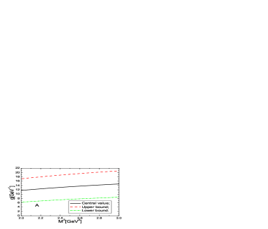
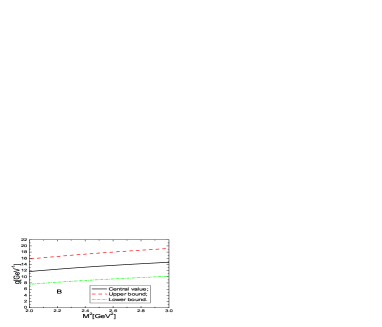
Figure 1: $g_{\Delta N\pi}$ with the Borel parameter $M^{2}$, $A$ for $a_{2}=0.25\pm 0.15$ and $B$ for $a_{2}=0.25\pm 0.08$.

The strong coupling constant $g_{\Delta N\pi}$ has the following relation with the decay width $\Gamma_{\Delta\to N\pi}$,

$$\Gamma_{\Delta\to N\pi} = \frac{g^{2}_{\Delta N\pi}p_{cm}}{32\pi M_{\Delta}^{2}}\sum_{ss^{\prime}}\mid\overline{U}(p^{\prime},s)p^{\mu}_{\pi}U_{\mu}(p^{\prime\prime},s^{\prime})\mid^{2}\,,$$

$$p_{cm} = \frac{\sqrt{[M_{\Delta}^{2}-(M_{p}+m_{\pi})^{2}][M_{\Delta}^{2}-(M_{p}-m_{\pi})^{2}]}}{2M_{\Delta}}\,.$$ (21)

If we take the experimental data as input parameter, $\Gamma_{\Delta\to N\pi}=118\,\rm{GeV}$ [1], we can obtain the value $g_{\Delta N\pi}\approx 15.6\,\rm{GeV}^{-1}$, our numerical result $g_{\Delta N\pi}=(13.5\pm 5.4)\,\rm{GeV}^{-1}$ is rather good.

In the region $M^{2}=(2.0-3.0)\,\rm{GeV}^{2}$, $\frac{\alpha_{s}(M)}{\pi}\sim 0.10-0.13$ [20]. If the radiative $\mathcal{O}(\alpha_{s})$ corrections to the leading perturbative terms are companied with large numerical factors, just like in the case of the QCD sum rules for the mass of the proton [19],

$$1+(\frac{53}{12}+\gamma_{E})\frac{\alpha_{s}(M)}{\pi}\sim 1+(0.54-0.65)\,,$$ (22)

the contributions of the order $\mathcal{O}(\alpha_{s})$ are large, neglecting them can impair the predictive ability. Furthermore, the pole residues $\lambda_{p}$ and $\lambda_{\Delta}$ also receive contributions from the perturbative $\mathcal{O}(\alpha_{s})$ corrections, if we take them into account properly, we can improve the value of the strong coupling constant $g_{\Delta N\pi}$.

4 Conclusion

In this article, we calculate the strong coupling constant $g_{\Delta N\pi}$ and study the strong decay $\Delta^{++}\to p\pi^{+}$ with the light-cone QCD sum rules. The numerical value of the strong coupling constant $g_{\Delta N\pi}$ is consistent with the experimental data. The small discrepancy maybe due to failure to take into account the perturbative $\mathcal{O}(\alpha_{s})$ corrections.

Appendix

The light-cone distribution amplitudes of the $\pi$ meson are defined by [10]

$$\langle 0|{\bar{u}}(x)\gamma_{\mu}\gamma_{5}d(0)|\pi(p)\rangle = if_{\pi}p_{\mu}\int_{0}^{1}due^{-iup\cdot x}\left\{\phi_{\pi}(u)+\frac{m_{\pi}^{2}x^{2}}{16}A(u)\right\}$$

$$+\frac{i}{2}f_{\pi}m_{\pi}^{2}\frac{x_{\mu}}{p\cdot x}\int_{0}^{1}due^{-iup\cdot x}B(u)\,,$$

$$\langle 0|{\bar{u}}(x)i\gamma_{5}d(0)|\pi(p)\rangle = \frac{f_{\pi}m_{\pi}^{2}}{m_{u}+m_{d}}\int_{0}^{1}due^{-iup\cdot x}\phi_{p}(u)\,,$$

$$\langle 0|{\bar{u}}(x)\sigma_{\mu\nu}\gamma_{5}d(0)|\pi(p)\rangle = i(x_{\mu}p_{\nu}-x_{\nu}p_{\mu})\frac{f_{\pi}m_{\pi}^{2}}{6(m_{u}+m_{d})}\int_{0}^{1}due^{-iup\cdot x}\phi_{\sigma}(u)\,,$$

$$\langle 0|{\bar{u}}(x)\sigma_{\mu\nu}\gamma_{5}g_{s}G_{\alpha\beta}(vx)d(0)|\pi(p)\rangle = f_{3\pi}\left\{(p_{\mu}p_{\alpha}g^{\bot}_{\nu\beta}-p_{\nu}p_{\alpha}g^{\bot}_{\mu\beta})-(p_{\mu}p_{\beta}g^{\bot}_{\nu\alpha}\right.$$

$$\left.-p_{\nu}p_{\beta}g^{\bot}_{\mu\alpha})\right\}\int{\cal D}\alpha_{i}\phi_{3\pi}(\alpha_{i})e^{-ip\cdot x(\alpha_{u}+v\alpha_{g})}\,,$$

$$\langle 0|{\bar{u}}(x)\gamma_{\mu}\gamma_{5}g_{s}G_{\alpha\beta}(vx)d(0)|\pi(p)\rangle = f_{\pi}m_{\pi}^{2}p_{\mu}\frac{p_{\alpha}x_{\beta}-p_{\beta}x_{\alpha}}{p\cdot x}$$

$$\int{\cal D}\alpha_{i}A_{\parallel}(\alpha_{i})e^{-ip\cdot x(\alpha_{u}+v\alpha_{g})}$$

$$+f_{\pi}m_{\pi}^{2}(p_{\beta}g^{\perp}_{\alpha\mu}-p_{\alpha}g^{\perp}_{\beta\mu})$$

$$\int{\cal D}\alpha_{i}A_{\perp}(\alpha_{i})e^{-ip\cdot x(\alpha_{u}+v\alpha_{g})}\,,$$

$$\langle 0|{\bar{u}}(x)\gamma_{\mu}ig_{s}\tilde{G}_{\alpha\beta}(vx)d(0)|\pi(p)\rangle = f_{\pi}m_{\pi}^{2}p_{\mu}\frac{p_{\alpha}x_{\beta}-p_{\beta}x_{\alpha}}{p\cdot x}$$ (23)

$$\int{\cal D}\alpha_{i}V_{\parallel}(\alpha_{i})e^{-ip\cdot x(\alpha_{u}+v\alpha_{g})}$$

$$+f_{\pi}m_{\pi}^{2}(p_{\beta}g^{\perp}_{\alpha\mu}-p_{\alpha}g^{\perp}_{\beta\mu})$$

$$\int{\cal D}\alpha_{i}V_{\perp}(\alpha_{i})e^{-ip\cdot x(\alpha_{u}+v\alpha_{g})}\,,$$

where $g_{\mu\nu}^{\perp}=g_{\mu\nu}-\frac{p_{\mu}x_{\nu}+p_{\nu}x_{\mu}}{p\cdot x}$, $\tilde{G}_{\mu\nu}=\frac{1}{2}\epsilon_{\mu\nu\alpha\beta}G^{\alpha\beta}$ and ${\cal{D}}\alpha_{i}=d\alpha_{u}d\alpha_{d}d\alpha_{g}\delta(1-\alpha_{u}-\alpha_{d}-\alpha_{g})$.

The light-cone distribution amplitudes of the $\pi$ meson are parameterized as [10]

$$\phi_{\pi}(u) = 6u(1-u)\left\{1+a_{1}C^{\frac{3}{2}}_{1}(\xi)+a_{2}C^{\frac{3}{2}}_{2}(\xi)\right\}\,,$$

$$\phi_{p}(u) = 1+\left\{30\eta_{3}-\frac{5}{2}\rho^{2}\right\}C_{2}^{\frac{1}{2}}(\xi)$$

$$+\left\{-3\eta_{3}\omega_{3}-\frac{27}{20}\rho^{2}-\frac{81}{10}\rho^{2}a_{2}\right\}C_{4}^{\frac{1}{2}}(\xi)\,,$$

$$\phi_{\sigma}(u) = 6u(1-u)\left\{1+\left[5\eta_{3}-\frac{1}{2}\eta_{3}\omega_{3}-\frac{7}{20}\rho^{2}-\frac{3}{5}\rho^{2}a_{2}\right]C_{2}^{\frac{3}{2}}(\xi)\right\}\,,$$

$$\phi_{3\pi}(\alpha_{i}) = 360\alpha_{u}\alpha_{d}\alpha_{g}^{2}\left\{1+\lambda_{3}(\alpha_{u}-\alpha_{d})+\omega_{3}\frac{1}{2}(7\alpha_{g}-3)\right\}\,,$$

$$V_{\parallel}(\alpha_{i}) = 120\alpha_{u}\alpha_{d}\alpha_{g}\left(v_{00}+v_{10}(3\alpha_{g}-1)\right)\,,$$

$$A_{\parallel}(\alpha_{i}) = 120\alpha_{u}\alpha_{d}\alpha_{g}a_{10}(\alpha_{d}-\alpha_{u})\,,$$

$$V_{\perp}(\alpha_{i}) = -30\alpha_{g}^{2}\left\{h_{00}(1-\alpha_{g})+h_{01}\left[\alpha_{g}(1-\alpha_{g})-6\alpha_{u}\alpha_{d}\right]\right.$$

$$\left.+h_{10}\left[\alpha_{g}(1-\alpha_{g})-\frac{3}{2}\left(\alpha_{u}^{2}+\alpha_{d}^{2}\right)\right]\right\}\,,$$

$$A_{\perp}(\alpha_{i}) = 30\alpha_{g}^{2}(\alpha_{u}-\alpha_{d})\left\{h_{00}+h_{01}\alpha_{g}+\frac{1}{2}h_{10}(5\alpha_{g}-3)\right\},$$

$$A(u) = 6u(1-u)\left\{\frac{16}{15}+\frac{24}{35}a_{2}+20\eta_{3}+\frac{20}{9}\eta_{4}\right.$$

$$+\left[-\frac{1}{15}+\frac{1}{16}-\frac{7}{27}\eta_{3}\omega_{3}-\frac{10}{27}\eta_{4}\right]C^{\frac{3}{2}}_{2}(\xi)$$

$$\left.+\left[-\frac{11}{210}a_{2}-\frac{4}{135}\eta_{3}\omega_{3}\right]C^{\frac{3}{2}}_{4}(\xi)\right\}+\left\{-\frac{18}{5}a_{2}+21\eta_{4}\omega_{4}\right\}$$

$$\left\{2u^{3}(10-15u+6u^{2})\log u+2\bar{u}^{3}(10-15\bar{u}+6\bar{u}^{2})\log\bar{u}\right.$$

$$\left.+u\bar{u}(2+13u\bar{u})\right\}\,,$$

$$g(u) = 1+g_{2}C^{\frac{1}{2}}_{2}(\xi)+g_{4}C^{\frac{1}{2}}_{4}(\xi)\,,$$

$$B(u) = g(u)-\phi_{\pi}(u)\,,$$ (24)

where

$$h_{00} = v_{00}=-\frac{\eta_{4}}{3}\,,$$

$$a_{10} = \frac{21}{8}\eta_{4}\omega_{4}-\frac{9}{20}a_{2}\,,$$

$$v_{10} = \frac{21}{8}\eta_{4}\omega_{4}\,,$$

$$h_{01} = \frac{7}{4}\eta_{4}\omega_{4}-\frac{3}{20}a_{2}\,,$$

$$h_{10} = \frac{7}{2}\eta_{4}\omega_{4}+\frac{3}{20}a_{2}\,,$$

$$g_{2} = 1+\frac{18}{7}a_{2}+60\eta_{3}+\frac{20}{3}\eta_{4}\,,$$

$$g_{4} = -\frac{9}{28}a_{2}-6\eta_{3}\omega_{3}\,,$$ (25)

$\xi=2u-1$, and $C_{2}^{\frac{1}{2}}(\xi)$, $C_{4}^{\frac{1}{2}}(\xi)$, $C_{1}^{\frac{3}{2}}(\xi)$, $C_{2}^{\frac{3}{2}}(\xi)$ are Gegenbauer polynomials, $\eta_{3}=\frac{f_{3\pi}}{f_{\pi}}\frac{m_{u}+m_{d}}{m_{\pi}^{2}}$ and $\rho^{2}={(m_{u}+m_{d})^{2}\over m_{\pi}^{2}}$ [4, 10, 17].

References

[1] W.-M. Yao et al, J. Phys. G33 (2006) 1.
[2] T. R. Hemmert, B. R. Holstein and J. Kambor, J. Phys. G24 (1998) 1831.
[3] T. M. Aliev, A. Ozpineci and M. Savci, Phys. Rev. D64 (2001) 034001; T. Doi, Y. Kondo and M. Oka, Phys. Rept. 398 (2004) 253; T. M. Aliev, A. Ozpineci, S. B. Yakovlev and V.
Zamiralov, Phys. Rev. D74 (2006) 116001; Z. G. Wang, Phys.
Rev. D75 (2007) 054020; and references therein.
[4]
I. I. Balitsky, V. M. Braun and A. V. Kolesnichenko, Nucl. Phys.
B312 (1989) 509; V. L. Chernyak and I. R. Zhitnitsky, Nucl.
Phys. B345 (1990) 137; V. L. Chernyak and A. R. Zhitnitsky,
Phys. Rept. 112 (1984) 173; V. M. Braun and I. E. Filyanov, Z.
Phys. C44 (1989) 157; V. M. Braun and I. E. Filyanov, Z.
Phys. C48 (1990) 239.
[5]
V. M. Braun, hep-ph/9801222; P. Colangelo and A. Khodjamirian,
hep-ph/0010175.
[6] M. A. Shifman, A. I. Vainshtein and V. I. Zakharov,
Nucl. Phys. B147 (1979) 385, 448; L. J. Reinders, H.
Rubinstein and S. Yazaki, Phys. Rept. 127 (1985) 1; S.
Narison, QCD Spectral Sum Rules, World Scientific Lecture Notes in
Physics 26 (1989) 1.
[7] B. L. Ioffe, Nucl. Phys. B188 (1981) 317; B. L.
Ioffe and A. V. Smilga, Nucl. Phys. B232 (1984) 109; V. M.
Belyaev and B. L. Ioffe, Sov. Phys. JETP 56 (1982) 493; V. M.
Belyaev and B. L. Ioffe, Sov. Phys. JETP 57 (1983) 716.
[8] V. Chung, H. G. Dosch, M. Kremer and D. Scholl,
Nucl. Phys. B197 (1982) 55; H. G. Dosch, M. Jamin and S.
Narison, Phys. Lett. B220 (1989) 251.
[9] V. M. Braun, A. Lenz, G. Peters and A. V. Radyushkin, Phys. Rev. D73 (2006) 034020.
[10] P. Ball, JHEP 9901 (1999) 010;
P. Ball and R. Zwicky, Phys. Lett. B633 (2006) 289;
P. Ball and R. Zwicky, JHEP 0602 (2006) 034;
P. Ball, V. M. Braun and A. Lenz,
JHEP 0605 (2006) 004.
[11]L. Li, Z. G. Wang and T. Huang, Phys. Rev. D70 (2004)
074006; B. Melic, Phys. Lett. B591 (2004) 91.
[12] Z. G. Wang, J. Phys. G34 (2007) 753.
[13] Z. G. Wang, Nucl. Phys. A796 (2007) 61.
[14] Z. G. Wang, J. Phys. G34 (2007)
493.
[15] V. A. Beilin and A. V. Radyushkin, Nucl. Phys. B260 (1985) 61;
P. Ball and V. M. Braun, Phys. Rev. D49 (1994) 2472;
V. A. Nesterenko and A. V. Radyushkin, Phys. Lett. B115 (1982) 410;
H. Kim, S. H. Lee and M. Oka, Prog. Theor. Phys. 109 (2003)
371.
[16] Z. H. Li, T. Huang, J. Z. Sun and Z. H. Dai, Phys. Rev. D65 (2002) 076005.
[17]
V. M. Belyaev, V. M. Braun, A. Khodjamirian and R. Rückl, Phys.
Rev. D51 (1995) 6177.
[18] B. L. Ioffe and K. N. Zyablyuk, Nucl. Phys.
A687 (2001) 437; B. V. Geshkenbein, B. L. Ioffe and K. N.
Zyablyuk, Phys. Rev. D64 (2001) 093009; B. L. Ioffe and K. N.
Zyablyuk, Eur. Phys. J. C27 (2003) 229; K. Zyablyuk, JHEP
0301 (2003) 081.
[19] B. L. Ioffe, Prog. Part. Nucl. Phys. 56 (2006)
232; and references therein.
[20] M. Davier, A. Hocker and Z. Zhang, Rev. Mod. Phys. 78 (2006) 1043;
and references therein.
[21] R. A. Arndt, W. J. Briscoe, I. I. Strakovsky and R. L. Workman, Phys. Rev. C74 (2006) 045205.