Relating two Hopf algebras built from an operad

Abstract

Starting from an operad, one can build a family of posets. From this family of posets, one can define an incidence Hopf algebra. By another construction, one can also build a group directly from the operad. We then consider its Hopf algebra of functions. We prove that there exists a surjective morphism from the latter Hopf algebra to the former one. This is illustrated by the case of an operad built on rooted trees, the $\operatorname{NAP}$ operad, where the incidence Hopf algebra is identified with the Connes-Kreimer Hopf algebra of rooted trees.

1 Introduction

Operads were introduced in algebraic topology to deal with loop spaces, more than 40 years ago. This new algebraic notion has been somewhat neglected after its introduction, until it appears to be useful in many other domains, for instance in the algebraic geometry of moduli spaces of curves, during the 1990’s. Since then, there seems to be a regular activity around operads.

Operads can be defined as objects of any symmetric monoidal category. Most of the examples considered in the literature live in the category of sets, of topological spaces, of vector spaces over a field, or of chain complexes.

The aim of the present article is to relate two different constructions, both starting from the data of an operad $\mathcal{P}$ in the category of sets, of graded commutative Hopf algebras or, from the dual point of view, of pro-algebraic groups.

The first construction goes as follows. From an operad $\mathcal{P}$ in the category of sets, one can define a family of posets, in which the partial order reflects part of the algebraic structure of the operad. This partial order has been introduced by Mendez and Yang [13] but rather in the context of species and without using the term operad; it was rediscovered later by Vallette [17], who used this to link the Koszul property of the operad to the Cohen-Macaulay properties of the posets.

Then, one can use this family of posets, which has some adequate closure property under taking subintervals, as an input to the Schmitt definition of an incidence Hopf algebra. Therefore, one can build in this way a first Hopf algebra $H_{\mathcal{P}}$ from an operad $\mathcal{P}$, through the associated posets.

The second construction of a Hopf algebra from an operad is a direct one. It is rather the equivalent construction of a pro-algebraic group $G_{\mathcal{P}}$. This has been considered, from different point of views in [18, 3, 10]. As a space, the group $G_{\mathcal{P}}$ is an affine subspace of the completed free $\mathcal{P}$-algebra on one generator.

Our main general result is the existence of a surjective morphism of Hopf algebras from the Hopf algebra of functions $\mathbb{Q}G_{\mathcal{P}}$ to the incidence Hopf algebra $H_{\mathcal{P}}$. From the group point of view, this means that the pro-algebraic group $\operatorname{Spec}H_{\mathcal{P}}$ is a subgroup of $G_{\mathcal{P}}$.

In the last section of the article, these results are applied to an operad built on rooted trees, the operad $\operatorname{NAP}$. We give a precise description of the posets associated to this operad. We then show that the incidence Hopf algebra for the $\operatorname{NAP}$ operad is isomorphic to the Hopf algebra of rooted trees which was introduced by Connes and Kreimer in [6]. This gives a second link between this Hopf algebra and operads, after the one obtained in [4] with the pre-Lie operad.

The general theorem is then used, together with a computation of the Möbius numbers, to find the inverse of a special element of $G_{\operatorname{NAP}}$. We also provide some other examples of elements of the group $G_{\operatorname{NAP}}$ and morphisms from this group to more familiar groups of formal power series in one variable.

The present work received support from the ANR grant BLAN06-1 136174.

2 Set-operads and posets

Here we recall first the general setting of species and operads, then the construction of posets starting from an operad (Mendez and Yang [13, §3.4] and Vallette [17]) and related results.

2.1 Species

The theory of species has been introduced by Joyal [9] as a natural way to deal with generating series. It is closely related to the notion of $\mathfrak{S}$-module, just as vector spaces are related to sets.

A species is a functor $\mathcal{P}$ from the groupoid of finite sets (the category whose objects are finite sets and morphisms are bijections) to the category of sets.

For example, the species $\operatorname{Comm}$ maps a finite set $I$ to the singleton $\{I\}$ and there is no choice for the bijections.

The category of species is a monoidal category with tensor product $\circ$ defined by

$$(F\circ G)(I)=\coprod_{\simeq}F(I/{\simeq})\times\prod_{J\in I/\simeq}G(J),$$

where $I$ is a finite set and $\simeq$ runs over the set of equivalence relations on $I$. Note that this monoidal functor is not symmetric.

The data of a species $\mathcal{P}$ is equivalent to the data of a collection of sets $\mathcal{P}(n)$ with actions of the symmetric groups. The set $\mathcal{P}(n)$ can be defined as $\mathcal{P}(\{1,\dots,n\})$, with the obvious action of the symmetric group $\mathfrak{S}_{n}$. The other way round, one can recover the set $\mathcal{P}(I)$ as a colimit.

2.2 Set-operads

A set-operad $\mathcal{P}$ is a monoid with unit in the monoidal category of species for the tensor product $\circ$. This means the data of a morphism of species

$$\gamma:\mathcal{P}\circ\mathcal{P}\to\mathcal{P},$$

which has to be associative, and a map $e$ from the unit object to $\mathcal{P}$ satisfying the usual unit axioms.

An augmented operad $\mathcal{P}$ is an operad such that $\mathcal{P}(\emptyset)$ is empty and the image by $\mathcal{P}$ of any singleton is a singleton. We will always assume that the operads we consider are augmented.

There is an alternative way to describe the composition map $\gamma$ of an operad $\mathcal{P}$. The data of $\gamma$ as above is equivalent to the data of maps, for each finite set $I$ and collection of finite sets $(J_{i})_{i\in I}$,

$$\mathcal{P}(I)\times\prod_{i\in I}\mathcal{P}(J_{i})\to\mathcal{P}(\coprod_{i\in I}J_{i}),$$ (1)

which map $(x,(y_{i})_{i\in I})$ to $x\boldsymbol{(}(y_{i})_{i\in I}\boldsymbol{)}$.

A basic set-operad is a set-operad such that, for each $y\in\prod_{i\in I}\mathcal{P}(J_{i})$, the map $x\mapsto x\boldsymbol{(}y\boldsymbol{)}$ is injective.

2.3 Posets from set-operads

Let $\mathcal{P}$ be a set-operad. Let us denote by $\Pi_{\mathcal{P}}$ the species $\operatorname{Comm}\circ\,\mathcal{P}$. Let $I$ be a finite set.

One can build a family of posets on the species $\Pi_{\mathcal{P}}$. More precisely, there is a partial order on $\Pi_{\mathcal{P}}(I)$ for each finite set $I$ and this construction is functorial in $I$. This means that the species $\Pi_{\mathcal{P}}$ has values in the category of posets rather than just in the category of sets.

From the definition of $\circ$, one can see that an element $x$ of $\Pi_{\mathcal{P}}(I)$ is the data of a partition $\pi_{x}$ of $I$ and of an element $x_{J}$ of $\mathcal{P}(J)$ for each part $J$ of the partition $\pi_{x}$. The definition of the composition maps of $\mathcal{P}$ in the diagram (1) lifts to the maps

$$\Pi_{\mathcal{P}}(I)\times\prod_{i\in I}\mathcal{P}(J_{i})\to\Pi_{\mathcal{P}}(\coprod_{i\in I}J_{i}),$$ (2)

which send $(x=(x_{u})_{u\in\pi_{x}},y=(y_{i})_{i\in I})$ to

$$x\boldsymbol{(}y\boldsymbol{)}=(x_{u}\boldsymbol{(}(y_{i})_{i\in u}\boldsymbol{)})_{u\in\pi_{x}}.$$

These maps satisfy the following associativity relation

$$x\boldsymbol{(}{y\boldsymbol{(}z\boldsymbol{)}}\boldsymbol{)}={x\boldsymbol{(}y\boldsymbol{)}}\boldsymbol{(}{z}\boldsymbol{)}.$$ (3)

Then $x\leq y$ in $\Pi_{\mathcal{P}}(I)$ if there exists an element $\theta(x,y)\in\Pi_{\mathcal{P}}(\pi_{x})$ such that

$$\theta(x,y)\boldsymbol{(}x\boldsymbol{)}=y.$$

Note that this definition implies that the partition $\pi_{x}$ is finer than the partition $\pi_{y}$.

The poset $\Pi_{\mathcal{P}}(I)$ has a unique minimal element, denoted by $\widehat{0}$.

The following proposition is statement 3. in [13, Thm. 3.4].

Proposition 2.1

Let $\mathcal{P}$ be a basic set-operad. Let $x\in\Pi_{\mathcal{P}}(I)$. The poset $\{y\in\Pi_{\mathcal{P}}(I)|\ x\leq y\}$ is isomorphic to the poset $\Pi_{\mathcal{P}}(\pi_{x})$.

• Proof. Since $\mathcal{P}$ is a basic set-operad, if $x\leq y$ there is a unique $\theta(x,y)\in\Pi_{\mathcal{P}}(\pi_{x})$ such that $\theta(x,y)\boldsymbol{(}x\boldsymbol{)}=y$. The bijection sends $y$ to $\theta(x,y)$. The inverse map sends $a\in\Pi_{\mathcal{P}}(\pi_{x})$ to $a\boldsymbol{(}x\boldsymbol{)}$. Assume $x\leq y\leq z$. By definition $\theta(x,y)\boldsymbol{(}x\boldsymbol{)}=y$ and $\theta(x,z)\boldsymbol{(}x\boldsymbol{)}=z$. Since $y\leq z$ there is a unique $\theta(y,z)\in\Pi_{\mathcal{P}}(\pi_{y})$ such that $\theta(y,z)\boldsymbol{(}y\boldsymbol{)}=z$. As a consequence, using the associativity relation (3), one has

  $$z=\theta(y,z)\boldsymbol{(}y\boldsymbol{)}=\theta(y,z)\boldsymbol{(}\theta(x,y)\boldsymbol{(}x\boldsymbol{)}\boldsymbol{)}=\theta(y,z)\boldsymbol{(}\theta(x,y)\boldsymbol{)}\boldsymbol{(}x\boldsymbol{)}=\theta(x,z)\boldsymbol{(}x\boldsymbol{)}.$$

  The uniqueness of the elements $\theta$ permits to conclude that $\theta(y,z)\boldsymbol{(}\theta(x,y)\boldsymbol{)}=\theta(x,z)$ and $\theta(x,y)\leq\theta(x,z).$

  Conversely, if $a\leq b\in\Pi_{\mathcal{P}}(\pi_{x})$ one has clearly $a\boldsymbol{(}x\boldsymbol{)}\leq b\boldsymbol{(}x\boldsymbol{)}$.  

If this construction is applied to the set-operad $\operatorname{Comm}$, the poset $\Pi_{\operatorname{Comm}}(I)$ is the usual partial order by refinement on the partitions of the set $I$.

One can similarly get the poset of pointed-partitions, when this construction is applied to the set-operad $\operatorname{Perm}$ [5].

Vallette has used these posets to give a Koszulness criteria for operads. Let us just recall the result here.

Proposition 2.2 ([17], Theorem 12)

Let $\mathcal{P}$ be a set-operad which is basic, quadratic and augmented. Then the associated linear operad $\mathbb{Q}\mathcal{P}$ is Koszul if and only if all maximal intervals in $\Pi_{\mathcal{P}}(I)$ are Cohen-Macaulay for all $I$.

3 Incidence Hopf algebras

Here we recall briefly a construction of William Schmitt [15] building a commutative Hopf algebra from a family of posets satisfying some conditions. We then derive our first Hopf algebra built from an operad from the composition of the construction of Mendez-Yang and Vallette with this construction of Schmitt.

3.1 Good families of posets

Suppose we are given a collection of posets $(P_{\alpha})_{\alpha\in\mathtt{A}}$. The collection $(P_{\alpha})_{\alpha\in\mathtt{A}}$ is called a good collection if it satisfies the following conditions.

1. Each poset $P_{\alpha}$ has a minimal element $\widehat{0}$ and a maximal element $\widehat{1}$ (it is an interval).

2. For all $\alpha\in\mathtt{A}$ and all $x$ in $P_{\alpha}$, the interval $[\widehat{0},x]$ is isomorphic to a product of posets $\prod_{\beta}P_{\beta}$ and the interval $[x,\widehat{1}]$ is isomorphic to a product of posets $\prod_{\gamma}P_{\gamma}$.

As a simple example of good collection, one can consider the family of all total orders. Another example is the family of boolean posets.

Remark: it follows from this definition applied to the interval $[\widehat{0},\widehat{0}]$ in any poset $P_{\alpha}$ that a good collection contains at least one poset $P_{\varepsilon}$ with only one element.

3.2 Hopf algebra from a good collection

Let $(P_{\alpha})_{\alpha\in\mathtt{A}}$ be a good collection. Let us consider the collection of all finite products $\prod_{\beta}P_{\beta}$. Let us denote by $\bar{\mathtt{A}}$ this larger set of posets.

The collection $\bar{\mathtt{A}}$ of posets is closed under products by construction. It is also closed under taking initial intervals $[\widehat{0},x]$ or final intervals $[x,\widehat{1}]$. Hence it is also closed under taking any subinterval, because any interval $[x,y]$ is a final interval in the initial interval $[\widehat{0},y]$.

A collection of posets which is closed under products and closed under taking subintervals is called a hereditary collection in [15]. The collection $\bar{\mathtt{A}}$ is therefore a hereditary collection.

Let us denote by $[\mathtt{A}]$ the set of isomorphism classes of posets in $\mathtt{A}$, and by $[\bar{\mathtt{A}}]$ the set of isomorphism classes of posets in $\bar{\mathtt{A}}$. Elements in these sets will be denoted by $[\alpha],[\beta],\dots$, which will also mean the isomorphism class of $\alpha,\beta,\dots\in\mathtt{A}$ or $\bar{\mathtt{A}}$.

One can then consider the vector space $H_{\mathtt{A}}$ with a basis $\mathsf{F}_{[\alpha]}$ indexed by the set $[\bar{\mathtt{A}}]$.

Then $H_{\mathtt{A}}$ is a commutative algebra for the product induced by the direct product of posets:

$$\mathsf{F}_{[\alpha]}\mathsf{F}_{[\beta]}=\mathsf{F}_{[\alpha\times\beta]}.$$

This algebra is generated by the elements $\mathsf{F}_{[\alpha]}$ with $[\alpha]\in[\mathtt{A}]$. Note that one can remove the unit $\mathsf{F}_{[\varepsilon]}$ from this set of generators. The algebra $H_{\mathtt{A}}$ may not be free on this reduced set of generators, as there can be isomorphisms $\prod_{\beta}P_{\beta}\simeq\prod_{\gamma}P_{\gamma}$ with a different number of factors or with non pairwise-isomorphic factor posets.

The space $H_{\mathtt{A}}$ is also a coalgebra for a coproduct $\Delta$ whose value on the generator $\mathsf{F}_{[\alpha]}$ is

$$\Delta(\mathsf{F}_{[\alpha]})=\sum_{x\in P_{\alpha}}\mathsf{F}_{[\widehat{0},x]}\otimes\mathsf{F}_{[x,\widehat{1}]},$$

where the intervals in indices stand for their isomorphism classes.

In fact, this formula is enough to define the coproduct $\Delta$, which is compatible with the product on $H_{\mathtt{A}}$.

To summarize,

Proposition 3.1

The space $H_{\mathtt{A}}$ endowed with its commutative product and the coproduct $\Delta$ is a commutative Hopf algebra. The unit is $\mathsf{F}_{[\varepsilon]}$, where $[\epsilon]$ is the isomorphism class of the singleton interval.

This is a consequence of the general theorem of Schmitt on hereditary collections of posets [15, Theorem 4.1].

3.3 Group from a good family

The commutative Hopf algebra $H_{\mathtt{A}}$ is the space of functions on a pro-algebraic group $\operatorname{Spec}H_{\mathtt{A}}$, the elements of which can be seen as some formal power series indexed by elements of $[\mathtt{A}]$. The fact that $H_{\mathtt{A}}$ is not necessarily a polynomial algebra on the set $(\mathsf{F}_{[\alpha]})_{[\alpha]\in[\mathtt{A}]}$ is equivalent to the possible existence of some universal relations between the coefficients of these series (see Lemma 6.12 for an instance of this phenomenon). The fact that $\mathsf{F}_{[\varepsilon]}$ is the unit means that the coefficient of $[\varepsilon]$ in these series is $1$.

An element of this pro-algebraic group can be considered as a function on the collection of isomorphism classes of posets $(P_{[\alpha]})_{[\alpha]\in[\mathtt{A}]}$. The product in the group provides information on the posets, by the classical theory of Möbius functions, zeta functions and incidence algebra of posets, see [14, 16].

The following proposition gives an example of computation in the pro-algebraic group $\operatorname{Spec}H_{\mathtt{A}}$.

Proposition 3.2 ([15] §7)

The group product in $\operatorname{Spec}H_{\mathtt{A}}$ gives the usual convolution product on functions over the posets $P_{[\alpha]}$ for $[\alpha]\in[\mathtt{A}]$. Consider in $\operatorname{Spec}H_{\mathtt{A}}$ the Möbius series

$$\mathtt{M}=\sum_{[\alpha]\in[\mathtt{A}]}\mu(P_{[\alpha]})[\alpha],$$

where $\mu(P_{[\alpha]})$ is the Möbius number of the poset $P_{[\alpha]}$, and the Zeta series

$$\mathtt{Z}=\sum_{[\alpha]\in[\mathtt{A}]}[\alpha].$$

Then $\mathtt{M}$ is the inverse of $\mathtt{Z}$ in $\operatorname{Spec}H_{\mathtt{A}}$.

3.4 From operads to incidence Hopf algebras

Here we show that one can use the posets $\Pi_{\mathcal{P}}(I)$ associated with a basic set-operad $\mathcal{P}$ to define an incidence Hopf algebra $H_{\mathcal{P}}$ by using Schmitt construction for an hereditary family.

Indeed the intervals in $\Pi_{\mathcal{P}}(I)$ are products of minimal intervals as stated in the following proposition.

Proposition 3.3

Let $y\in\mathcal{P}(n)$ for some $n$. Let $\widehat{0}\leq x\leq y$. Assume that $x$ has components $(x_{u})_{u\in\pi_{x}}$. The interval $[\widehat{0},x]$ is isomorphic to the product of posets $\prod_{u\in\pi_{x}}[\widehat{0},x_{u}]$. The interval $[x,\widehat{1}]=[x,y]$ is isomorphic to the poset $[\widehat{0},\theta(x,y)]$, where $\theta(x,y)$ is the unique element of $\mathcal{P}(\pi_{x})$ such that $\theta(x,y)\boldsymbol{(}x\boldsymbol{)}=y$.

• Proof. The isomorphism between $[\widehat{0},x]$ and $\prod_{u\in\pi_{x}}[\widehat{0},x_{u}]$ is a direct consequence of the definition of the partial order. Indeed, one has $z\leq x$ if and only if the partition $\pi_{z}$ is finer than the partition $\pi_{x}$ and for each part $u$ of $\pi_{x}$, one has $z_{u}\leq x_{u}$, where $z_{u}$ and $x_{u}$ are the restrictions of $z$ and $x$ to $u$. This allows to prove the expected isomorphism.

  Let us now consider the interval $[x,y]$. The order preserving isomorphism of Prop. 2.1 between $\{z|x\leq z\}$ and $\Pi_{\mathcal{P}}(\pi_{x})$ induces an isomorphism between the intervals $[x,y]$ and $[\widehat{0},\theta(x,y)]$.  

As a consequence, if $x\leq y\in\Pi_{\mathcal{P}}(I)$ and $y=(y_{u})_{u\in\pi_{y}}$ then

$$[x,y]\simeq\prod_{u\in\pi_{y}}[\widehat{0},\theta(x_{u},y_{u})].$$ (4)

Let $\mathtt{A}_{\mathcal{P}}$ be the set of coinvariants for the species $\mathcal{P}$. For each coinvariant $\alpha\in\mathcal{P}(n)_{\mathfrak{S}n}$, let $r(\alpha)$ be a representative of $\alpha$ in $\mathcal{P}(n)$. Let us define a poset $P_{\alpha}$ as the interval $[\widehat{0},r(\alpha)]$ in $\Pi_{\mathcal{P}}(n)$.

Proposition 3.4

The collection of posets $(P_{\alpha})_{\alpha\in{\mathtt{A}_{\mathcal{P}}}}$ is a good family of posets. The resulting incidence Hopf algebra is denoted by $H_{\mathcal{P}}$.

• Proof. Obviously, all posets $P_{\alpha}$ are intervals. There remains only to prove the stability property. For any $\alpha\in\mathtt{A}_{\mathcal{P}}$, two representatives $r(\alpha)$ and $s(\alpha)$ give two isomorphic intervals $[\widehat{0},r(\alpha)]$ and $[\widehat{0},s(\alpha)]$ in $\Pi_{\mathcal{P}}(n)$. Thus, the stability property follows from Prop. 3.3.  

4 Groups from operads

Here we recall the construction of a group from an operad. The Hopf algebra of its functions gives our second Hopf algebra built from an operad.

We will work with a set-operad $\mathcal{P}$, but the construction is just the same for an operad in the category of vector spaces. This simple construction has already been considered from different viewpoints in [18, Chap. I, §1.2] and [3, 10].

Let $\mathcal{P}$ be an augmented set operad. In this section, we will use the description of a species $\mathcal{P}$ as a collection of modules $\mathcal{P}(n)$ over the symmetric groups.

Let $\mathbb{Q}\mathtt{A}_{\mathcal{P}}=\oplus_{n}\mathbb{Q}\mathcal{P}(n)_{\mathfrak{S}_{n}}$ be the direct sum of the coinvariant spaces, which can be identified with the underlying vector space of the free $\mathcal{P}$-algebra on one generator, and $\widehat{\mathbb{Q}\mathtt{A}}_{\mathcal{P}}={\prod}_{n}\mathbb{Q}\mathcal{P}(n)_{\mathfrak{S}_{n}}$ be its completion.

Let $\alpha=\sum_{m}\alpha_{m}$, $\beta=\sum_{n}\beta_{n}$ be two elements of $\widehat{\mathbb{Q}\mathtt{A}}_{\mathcal{P}}$ with $\alpha_{m},\beta_{m}$ elements of $\mathbb{Q}\mathcal{P}(m)_{\mathfrak{S}_{m}}$. Choose any representatives ${x}_{m}=r(\alpha_{m})$ of $\alpha_{m}$ (resp. ${y}_{m}=r(\beta_{m})$ of $\beta_{m}$) in $\mathbb{Q}\mathcal{P}(m)$. Then one can check that the following formula defines a product on $\widehat{\mathbb{Q}\mathtt{A}}_{\mathcal{P}}$:

$$\alpha\times\beta=\sum_{m\geq 1}\,\sum_{n_{1},\dots,n_{m}\geq 1}\langle{x}_{m}\boldsymbol{(}{y}_{n_{1}},\dots,{y}_{n_{m}}\boldsymbol{)}\rangle,$$ (5)

where $\langle\,\rangle$ is the quotient map to the coinvariants and $(x,y_{1},\dots,y_{m})\mapsto x\boldsymbol{(}y_{1},\dots,y_{m}\boldsymbol{)}$ is the composition map of the operad $\mathcal{P}$.

Proposition 4.1

The product $\times$ defines the structure of an associative monoid on the vector space $\widehat{\mathbb{Q}\mathtt{A}}_{\mathcal{P}}$. Furthermore, this product is $\mathbb{Q}$-linear on its left argument.

• Proof. Let us first prove the associativity. Let $\delta=\sum_{p}\delta_{p}$ and fix representatives $z_{p}=r(\delta_{p})$. On the one hand, one has

  $$(\alpha\times\beta)\times\delta=\sum_{m}\sum_{p_{1},\dots,p_{m}}\langle r((\alpha\times\beta)_{m})\boldsymbol{(}{z}_{p_{1}},\dots,{z}_{p_{m}}\boldsymbol{)}\rangle\\ =\sum_{m}\sum_{n_{1},\dots,n_{m}}\,\sum_{p_{1},\dots,p_{n_{1}+\dots+n_{m}}}\langle{x}_{m}\boldsymbol{(}{y}_{n_{1}},\dots,{y}_{n_{m}}\boldsymbol{)}\boldsymbol{(}{z}_{p_{1}},\dots,{z}_{p_{n_{1}+\dots+n_{m}}}\boldsymbol{)}\rangle.$$ (6)

  On the other hand, one has

  $$\alpha\times(\beta\times\delta)=\sum_{m}\sum_{n_{1},\dots,n_{m}}\langle{x}_{m}\boldsymbol{(}r((\beta\times\delta)_{n_{1}}),\dots,r((\beta\times\delta)_{n_{m}})\boldsymbol{)}\rangle\\ =\sum_{m}\sum_{n_{1},\dots,n_{m}}\sum_{(q_{i,j})}\langle{x}_{m}\boldsymbol{(}{y}_{n_{1}}\boldsymbol{(}{z}_{q_{1,1}},\dots,{z}_{q_{1,n_{1}}}\boldsymbol{)},\dots,{y}_{n_{m}}\boldsymbol{(}{z}_{q_{m,1}},\dots,{z}_{q_{m,n_{m}}}\boldsymbol{)}\boldsymbol{)}\rangle.$$ (7)

  Using then the “associativity” of the operad, one gets the associativity of $\times$. It is easy to check that the image $\varepsilon$ of the unit $e$ of the operad $\mathcal{P}$ is a two-sided unit for the $\times$ product. The left $\mathbb{Q}$-linearity is clear from the formula (5).  

Proposition 4.2

An element $\beta$ of $\widehat{\mathbb{Q}\mathtt{A}}_{\mathcal{P}}$ is invertible for $\times$ if and only if the first component $\beta_{1}$ of $\beta$ is non-zero.

• Proof. The direct implication is trivial. The converse is proved by a very standard recursive argument.  

Let us call $G_{\mathcal{P}}$ the set of elements of $\widehat{\mathbb{Q}\mathtt{A}}_{\mathcal{P}}$ whose first component is exactly the unit $\varepsilon$. This is a subgroup for the $\times$ product of the set of invertible elements.

Proposition 4.3

The construction $G$ is a functor from the category of augmented operads to the category of groups.

• Proof. The functoriality follows from inspection of the definitions of $\widehat{\mathbb{Q}\mathtt{A}}_{\mathcal{P}}$ and $\times$.  

In fact, one can see $G_{\mathcal{P}}$ as the group of $\mathbb{Q}$-points of a pro-algebraic and pro-unipotent group. The Lie algebra of this pro-algebraic group is given by the usual linearization process on the tangent space (an affine subspace of $\widehat{\mathbb{Q}\mathtt{A}}_{\mathcal{P}}$), resulting in the formula

$$[\alpha,\beta]=\sum_{m\geq 1}\sum_{n\geq 1}\langle{x}_{m}\circ{y}_{n}-{y}_{n}\circ{x}_{m}\rangle,$$

where

$${x}_{m}\circ{y}_{n}=\sum_{i=1}^{m}{x}_{m}\boldsymbol{(}\underbrace{e,\dots,e}_{i-1\text{ units}},{y}_{n},e,\dots,e\boldsymbol{)}.$$

The graded Lie algebra structure on $\mathbb{Q}\mathtt{A}_{\mathcal{P}}$ defined by the same formulas has already appeared in the work of Kapranov and Manin on the category of right modules over an operad [10, Th. 1.7.3].

The Hopf algebra $\mathbb{Q}[G_{\mathcal{P}}]$ of functions on $G_{\mathcal{P}}$ is the free commutative algebra generated by $\mathsf{G}_{\alpha}$ for $\alpha$ in the set $\mathtt{A}_{\mathcal{P}}$ but the unit invariant $\varepsilon$. An element $g$ of $G_{\mathcal{P}}$ can be seen as a formal sum

$$g=\sum_{\alpha\in\mathtt{A}_{\mathcal{P}}}\mathsf{G}_{\alpha}(g)\alpha,$$

where $\mathsf{G}_{\varepsilon}=1$. As a function on $G_{\mathcal{P}}$, the value of $\mathsf{G}_{\alpha}$ on an element $g$ of $G_{\mathcal{P}}$ is the coefficient of $\alpha$ in the expansion of $g$.

5 Main theorem

Here we show that the incidence Hopf algebra $H_{\mathcal{P}}$ defined in §3.4 is a quotient of the Hopf algebra of functions $\mathbb{Q}[G_{\mathcal{P}}]$ on the group of formal power series defined directly from the operad $\mathcal{P}$ by the construction of §4.

This also means that the group $\operatorname{Spec}H_{\mathcal{P}}$ is a subgroup of the group $G_{\mathcal{P}}$.

Let us consider the coproduct $\Delta$ in the incidence Hopf algebra $H_{\mathcal{P}}$. This space has a basis indexed by the set $[\bar{\mathtt{A}}_{\mathcal{P}}]$ of isomorphism classes of products of posets. The set $[\mathtt{A}_{\mathcal{P}}]$ is a subset of $[\bar{\mathtt{A}}_{\mathcal{P}}]$. If one considers the coproduct on one element $\mathsf{F}_{[\alpha]}$ with $\alpha\in[\mathtt{A}_{\mathcal{P}}]$, then it can be written uniquely as a linear combination

$$\Delta(\mathsf{F}_{[\alpha]})=\sum_{[\gamma],[\beta]}\mathbf{f}_{[\alpha]}^{[\beta],[\gamma]}\mathsf{F}_{[\beta]}\otimes\mathsf{F}_{[\gamma]},$$

where $([\alpha],[\beta],[\gamma])$ in $[\mathtt{A}_{\mathcal{P}}]\times[\bar{\mathtt{A}}_{\mathcal{P}}]\times[\mathtt{A}_{\mathcal{P}}]$. Indeed, the fact that this sum only runs over $\gamma\in[\mathtt{A}_{\mathcal{P}}]$ (and not $[\bar{\mathtt{A}}_{\mathcal{P}}]$) follows from the description of the subintervals in Prop. 3.3.

Therefore, for each triple $([\alpha],[\beta],[\gamma])$ in $[\mathtt{A}_{\mathcal{P}}]\times[\bar{\mathtt{A}}_{\mathcal{P}}]\times[\mathtt{A}_{\mathcal{P}}]$, one can define a coefficient $\mathbf{f}_{[\alpha]}^{[\beta],[\gamma]}$ by the previous expansion.

Similarly, one can consider the Hopf algebra of functions on the group $G_{\mathcal{P}}$ and define, for each triple $(\alpha,\beta,\gamma)$ with $\alpha$ an element of $\mathcal{P}(n)_{\mathfrak{S}_{n}}$ for some $n$, $\gamma$ an element of $\mathcal{P}(k)_{\mathfrak{S}_{k}}$ for some $k\leq n$ and $\beta$ an element of $(\Pi_{\mathcal{P}})(n)_{\mathfrak{S}_{n}}$ with $k$ parts, a coefficient $\mathbf{g}_{\alpha}^{\beta,\gamma}$ by

$$\Delta(\mathsf{G}_{\alpha})=\sum_{\gamma,\beta}\mathbf{g}_{\alpha}^{\beta,\gamma}\mathsf{G}_{\beta}\otimes\mathsf{G}_{\gamma},$$

where $\mathsf{G}_{\beta}$ is the product $\prod_{t}\mathsf{G}_{\beta_{t}}$ over the set of components of $\beta$.

Let us choose for the rest of this section a triple $(\alpha,\beta,\gamma)$ as above. We will compare the coefficients $\mathbf{f}_{[\alpha]}^{[\beta],[\gamma]}$ and $\mathbf{g}_{\alpha}^{\beta,\gamma}$.

Let us denote by $\langle\,\rangle$ the projections to coinvariants from $\mathcal{P}(n)$ to $\mathcal{P}(n)_{\mathfrak{S}_{n}}$.

Let us pick a representative $r(\alpha)$ of $\alpha$ in $\mathcal{P}(n)$ and a representative $r(\gamma)$ of $\gamma$ in $\mathcal{P}(k)$. Let us also choose a representative $r(\beta)$ of $\beta$ in $(S^{k}\mathcal{P})(n)$ with the following property: the partition of $\{1,\dots,n\}$ induced by the components of the representative $r(\beta)$ is the standard partition

$$p_{\operatorname{std}}=\{1,\dots,\ell_{1}\}\sqcup\{\ell_{1}+1,\dots,\ell_{1}+\ell_{2}\}\sqcup\dots\sqcup\{\ell_{1}+\dots+\ell_{k-1}+1,\dots,\ell_{1}+\dots+\ell_{k}\}.$$

This allows to define a bijection between the set of components of $\beta$ and the set $\{1,\dots,k\}$. Then one will denote by $\beta_{i}$ the component indexed by $i$. By the unique increasing renumbering, this also gives representatives $r(\beta_{i})$ of $\beta_{i}$ in $\mathcal{P}(\ell_{i})$.

Let us introduce the automorphism groups $\operatorname{Aut}(\alpha)$, $\operatorname{Aut}(\gamma)$ and $\operatorname{Aut}(\beta)$. They are rather the automorphisms groups of representatives $r(\alpha)$, $r(\beta)$ and $r(\gamma)$. The group $\operatorname{Aut}(\beta)$ decomposes into a semi-direct product

$$\operatorname{Aut}(\beta)=\left(\prod_{i=1}^{k}\operatorname{Aut}(\beta_{i})\right)\rtimes\operatorname{Aut}_{0}(\beta),$$

where $\operatorname{Aut}_{0}(\beta)$ is a subgroup of the permutation group $\mathfrak{S}_{k}$ of the set of components of $\beta$.

From the description of the coproduct in the incidence Hopf algebra, the coefficient $\mathbf{f}_{[\alpha]}^{[\beta],[\gamma]}$ is the cardinal number of the following set

$$\{p,\sigma\in\mathfrak{S}_{k},u,v_{i}\mid r(\alpha)=u\boldsymbol{(}v_{1},\dots,v_{k}\boldsymbol{)},\quad\langle u\rangle=\gamma,\quad\langle v_{\sigma(i)}\rangle=\beta_{i}\},$$ (8)

where $p$ is a partition of $\{1,\dots,n\}$ with $k$ parts $p_{i}$ ordered by their least element, $\sigma\in\mathfrak{S}_{k}$, $u\in\mathcal{P}(k)$ and $v_{i}\in\mathcal{P}(p_{i})$ for $i=1,\dots,k$.

Let us introduce the set $\mathtt{E}_{\mathbf{f}}(\alpha,\beta,\gamma)$ consisting of

$$\{p,\sigma,\psi,\phi_{i},u,v_{i}\mid r(\alpha)=u\boldsymbol{(}v_{1},\dots,v_{k}\boldsymbol{)},\quad u\simeq^{\psi}r(\gamma),\quad v_{\sigma(i)}\simeq^{\phi_{i}}r(\beta_{i})\}$$

where $p$ is a partition of $\{1,\dots,n\}$ with $k$ parts $p_{i}$ ordered by their least element, $\sigma\in\mathfrak{S}_{k}$, $u\in\mathcal{P}(k)$, $v_{i}\in\mathcal{P}(p_{i})$ for $i=1,\dots,k$, $\psi\in\mathfrak{S}_{k}$ and $\phi_{i}$ is bijection from the part $p_{\sigma(i)}$ to the set $\{1,\dots,\ell_{i}\}$.

Proposition 5.1

The set $\mathtt{E}_{\mathbf{f}}(\alpha,\beta,\gamma)$ satisfies

$$\operatorname{\#Aut}(\beta)\operatorname{\#Aut}(\gamma)\,\mathbf{f}_{[\alpha]}^{[\beta],[\gamma]}=\#\mathtt{E}_{\mathbf{f}}(\alpha,\beta,\gamma).$$

• Proof. The group $\operatorname{Aut}(\beta)\times\operatorname{Aut}(\gamma)$ acts freely on $\mathtt{E}_{\mathbf{f}}(\alpha,\beta,\gamma)$ and the orbits are in bijection with the set described in (8) whose cardinality is $\mathbf{f}_{[\alpha]}^{[\beta],[\gamma]}$.  

From the description of the product in the group $G_{\mathcal{P}}$, the coefficient $\mathbf{g}_{\alpha}^{\beta,\gamma}$ is the cardinal of the following set

$$\{\tau\in\mathfrak{S}_{k}/\operatorname{Aut}_{0}(\beta)\mid\alpha=\langle r(\gamma)\boldsymbol{(}r(\beta_{\tau(1)}),\dots,r(\beta_{\tau(k)})\boldsymbol{)}\rangle\}.$$ (9)

Let us introduce the set $\mathtt{E}_{\mathbf{g}}(\alpha,\beta,\gamma)$ consisting of

$$\{\tau\in\mathfrak{S}_{k},\phi\in\mathfrak{S}_{n}\mid r(\alpha)\simeq^{\phi}r(\gamma)\boldsymbol{(}r(\beta_{\tau(1)}),\dots,r(\beta_{\tau(k)})\boldsymbol{)}\}).$$

Proposition 5.2

The set $\mathtt{E}_{\mathbf{g}}(\alpha,\beta,\gamma)$ satisfies

$$\operatorname{\#Aut}(\alpha)\operatorname{\#Aut}_{0}(\beta)\,\mathbf{g}_{\alpha}^{\beta,\gamma}=\#\mathtt{E}_{\mathbf{g}}(\alpha,\beta,\gamma).$$

• Proof. The group $\operatorname{Aut}(\alpha)\times\operatorname{Aut}_{0}(\beta)$ acts freely on $\mathtt{E}_{\mathbf{g}}(\alpha,\beta,\gamma)$ and the orbits are in bijection with the set described in (9) whose cardinality is $\mathbf{g}_{\alpha}^{\beta,\gamma}$.  

Let us now show that the sets $\mathtt{E}_{\mathbf{f}}$ and $\mathtt{E}_{\mathbf{g}}$ are just the same.

Proposition 5.3

There is a bijection between $\mathtt{E}_{\mathbf{f}}(\alpha,\beta,\gamma)$ and $\mathtt{E}_{\mathbf{g}}(\alpha,\beta,\gamma)$.

• Proof. Recall the definition of the set $\mathtt{E}_{\mathbf{f}}(\alpha,\beta,\gamma)$ consisting of

  $$\{p,\sigma,\psi,\phi_{i},u,v_{i}\mid r(\alpha)=u\boldsymbol{(}v_{1},\dots,v_{k}\boldsymbol{)},\quad u\simeq^{\psi}r(\gamma),\quad v_{\sigma(i)}\simeq^{\phi_{i}}r(\beta_{i})\}.$$

  Let us pick an element in this set. Then there exists a unique permutation $\phi\in\mathfrak{S}_{n}$ induced by the collection of bijections $\phi_{i}$. This bijection maps the partition $p$ to the standard partition $p_{\operatorname{std}}$, changing the order of the parts according to $\sigma$. It provides an isomorphism between $r(\alpha)$ and

  $$\sigma^{-1}(u)\boldsymbol{(}r(\beta_{1}),\dots,r(\beta_{k})\boldsymbol{)}.$$

  Then one can use $\psi$ and $\sigma^{-1}$ to define a unique isomorphism $\tau$ between $\sigma^{-1}(u)$ and $r(\gamma)$. This gives us an equality

  $$\sigma^{-1}(u)\boldsymbol{(}r(\beta_{1}),\dots,r(\beta_{k})\boldsymbol{)}=r(\gamma)\boldsymbol{(}r(\beta_{\tau(1)}),\dots,r(\beta_{\tau(k)})\boldsymbol{)},$$

  hence a unique element in the set

  $$\mathtt{E}_{\mathbf{g}}(\alpha,\beta,\gamma)=\{\tau\in\mathfrak{S}_{k},\phi\in\mathfrak{S}_{n}\mid r(\alpha)\simeq^{\phi}r(\gamma)\boldsymbol{(}r(\beta_{\tau(1)}),\dots,r(\beta_{\tau(k)}\boldsymbol{)}\}.$$

   

One can now prove the existence of a morphism between Hopf algebras or equivalently between groups.

Theorem 5.4

The map $\rho:\mathsf{G}_{\alpha}\mapsto\frac{\mathsf{F}_{[\alpha]}}{\operatorname{\#Aut}(\alpha)}$ defines a surjective morphism from the Hopf algebra $\mathbb{Q}[G_{\mathcal{P}}]$ of coordinates on the group $G_{\mathcal{P}}$ to the incidence Hopf algebra $H_{\mathcal{P}}$. In terms of groups, this means that the group $\operatorname{Spec}H_{\mathcal{P}}$ is a subgroup of the group $G_{\mathcal{P}}$.

• Proof. The Hopf algebra $\mathbb{Q}[G_{\mathcal{P}}]$ is commutative and freely generated by the set of coinvariants of $\mathcal{P}$ (but the unit). On the other hand, the incidence Hopf algebra is commutative and generated by the isomorphism classes of maximal intervals (but the trivial interval).

  As intervals coming from the same coinvariant are obviously isomorphic, the proposed map is well defined from the set of coinvariants to the set of isomorphism classes of intervals. Then one can uniquely extend this map into a morphism of algebras, because $\mathbb{Q}[G_{\mathcal{P}}]$ is a free commutative algebra. This morphism is surjective by construction.

  According to the notation introduced before, we have to prove that

  $$\operatorname{\#Aut}(\alpha)\,\mathbf{g}_{\alpha}^{\beta,\gamma}=\prod_{t}\operatorname{\#Aut}(\beta_{t})\operatorname{\#Aut}(\gamma)\,\mathbf{f}_{[\alpha]}^{[\beta],[\gamma]}.$$

  By the semi-direct product structure of $\operatorname{Aut}(\beta)$, this is equivalent to

  $$\operatorname{\#Aut}(\alpha)\operatorname{\#Aut}_{0}(\beta)\,\mathbf{g}_{\alpha}^{\beta,\gamma}=\operatorname{\#Aut}(\beta)\operatorname{\#Aut}(\gamma)\,\mathbf{f}_{[\alpha]}^{[\beta],[\gamma]}.$$

  This follows in turn from Prop. 5.1, Prop. 5.2 and Prop. 5.3.  

Let us consider briefly a simple example, which is the operad $\operatorname{Comm}$. For each $n$, the space $\operatorname{Comm}(n)$ is the trivial module over the symmetric group $\mathfrak{S}_{n}$, hence $\operatorname{Comm}(n)_{\mathfrak{S}_{n}}$ has dimension $1$. The algebra of functions $\mathbb{Q}[G_{\operatorname{Comm}}]$ is free on one generator $\mathsf{G}_{n}$ in each degree $\geq 2$. Using the definition of $G_{\operatorname{Comm}}$, one can check that the group $G_{\operatorname{Comm}}$ is isomorphic to the group of formal power series

$$f=x+\sum_{n\geq 2}\mathsf{G}_{n}(f)x^{n}$$

for composition (a group of formal diffeomorphisms).

On the other hand, there is only one interval in $\Pi_{\operatorname{Comm}}(n)$, which is the usual poset of partitions. The incidence Hopf algebra of this family of posets is very classical [15, Ex. 14.1], freely generated by one element $\mathsf{F}_{n}$ in each degree and isomorphic to the Faà di Bruno Hopf algebra, which is the Hopf algebra of functions on the group of formal power series

$$f=x+\sum_{n\geq 2}\mathsf{F}_{n}(f)\frac{x^{n}}{n!}.$$

for composition.

Hence, in the case of $\operatorname{Comm}$, the morphism from $\mathbb{Q}[G_{\operatorname{Comm}}]$ to $H_{\operatorname{Comm}}$ which maps $\mathsf{G}_{n}$ to $\mathsf{F}_{n}/n!$ is an isomorphism. The next section is devoted to the case of the operad $\operatorname{NAP}$ where the surjective morphism is not an isomorphism.

6 Application to the $\operatorname{NAP}$ operad

6.1 The $\operatorname{NAP}$ operad

The us first recall the definition of the $\operatorname{NAP}$ operad, which has been introduced in [11]. The name $\operatorname{NAP}$ stands for ”non-associative permutative”.

Let $I$ be a finite set. The set $\operatorname{NAP}(I)$ is the set of rooted trees with vertices $I$, that is, connected and simply connected graphs with a distinguished vertex called the root. The unit is the unique rooted tree on the set $\{i\}$ for any singleton.

We use the notation

$$t=B(r,t_{1},\dots,t_{k})$$

for a rooted tree $t$ built from the rooted trees $t_{i}$ by adding an edge from the root of each rooted tree $t_{i}$ to a disjoint vertex $r$, which becomes the root of $t$.

Let us describe the composition $t\boldsymbol{(}(s_{i})_{i\in I}\boldsymbol{)}$, where $t\in\operatorname{NAP}(I)$ and $s_{i}\in\operatorname{NAP}(J_{i})$.

Consider the disjoint union of the rooted trees $s_{i}$ and add some edges: for each edge of $t$ between $i$ and $i^{\prime}$ in $I$, add an edge between the root of $s_{i}$ and the root of $s_{i^{\prime}}$. The result is a rooted tree on the vertices $\sqcup_{i}J_{i}$. This is $t\boldsymbol{(}(s_{i})_{i\in I}\boldsymbol{)}$. The root of this rooted tree is the root of $s_{k}$ where $k$ is the index of the root of $t$.

A $\operatorname{NAP}$-algebra is a vector space $V$ endowed with a bilinear map $\triangleleft$ from $V\otimes V\to V$ such that

$$(a\triangleleft b)\triangleleft c=(a\triangleleft c)\triangleleft b.$$

The free $\operatorname{NAP}$-algebra on a set $\mathtt{S}$ of generators has a basis indexed by rooted trees together with a bijection from vertices to $\mathtt{S}$. The product $s\triangleleft t$ of two such rooted trees is obtained by grafting the root of $t$ on the root of $s$: $B(r,s_{1},\ldots,s_{k})\triangleleft t=B(r,s_{1},\ldots,s_{k},t)$.

Let us note here that $\operatorname{NAP}$ is a basic set-operad. Indeed, one can recover $t$ from $u=t\boldsymbol{(}(s_{i})_{i\in I}\boldsymbol{)}$ and the collection $(s_{i})_{i\in I}$ as the restriction of $u$ to the vertices which are roots of some rooted tree $s_{i}$.

6.2 Posets associated with $\operatorname{NAP}$

Let us describe the posets $\Pi_{\operatorname{NAP}}(I)$. The set $\Pi_{\operatorname{NAP}}(I)$ consists of forests of rooted trees with vertices labeled by $I$.

The covering relations can be described as follows: a forest $x$ is covered by a forest $y$ if $y$ is obtained from $x$ by grafting the root of one component of $x$ on the root of another component of $x$. In the other direction, $x$ is obtained from $y$ by removing an edge incident to the root of one component of $y$.

By relation (4), any interval in $\Pi_{\operatorname{NAP}}(I)$ is a product of intervals of the form $[\widehat{0},t]$ for $t\in\operatorname{NAP}(J)$.

Let us introduce the following order on rooted trees: $t\leq_{s}t^{\prime}$ or $t^{\prime}$ is a sub-rooted tree of $t$ if $t^{\prime}$ is the restriction of $t$ to a subset of vertices containing the root of $t$, such that every vertex of $t$ lying on the path between the root and a vertex of $t^{\prime}$ is also in $t^{\prime}$. If $t$ itself is seen as a poset with its root as minimum element, then this just means that $t^{\prime}$ is a lower ideal of $t$.

Let $\widehat{1}$ denotes the root of $t$ and $[t,\widehat{1}]_{s}$ be the interval between $t$ and $\widehat{1}$ for the order $\leq_{s}$. A rooted tree $t$ is covered by a rooted tree $t^{\prime}$ if $t^{\prime}$ is obtained from $t$ by removing a leaf.

Proposition 6.1

The interval $[\widehat{0},t]$ is isomorphic to the interval $[t,\widehat{1}]_{s}$.

• Proof. Let $x$ be a forest such that $x\leq t$ and let $r_{x}$ be the family of its roots. By definition of the order relation, there exists a rooted tree $z$ such that $t=z\boldsymbol{(}x\boldsymbol{)}$. It means that the vertices indexed by $r_{x}$ form a sub-rooted tree of $t$. The isomorphism from $[\widehat{0},t]$ to $[t,\widehat{1}]_{s}$ sends $x$ to this sub-rooted tree. The inverse morphism is the following: let $t^{\prime}$ be a sub-rooted tree of $t$ and $r_{t^{\prime}}$ the set of its vertices. Again, in view of the composition, there is a unique forest $x\leq t$ whose roots are indexed by $r_{t^{\prime}}$ such that $t=t^{\prime}\boldsymbol{(}x\boldsymbol{)}$.  

This proposition in fact shows that $[\widehat{0},t]$ is isomorphic to the lattice of lower order ideals of the rooted tree $t$ seen as a poset. From this, it follows that $[\widehat{0},t]$ is a distributive lattice ([1]). According to [12, Example 2.4]), this also implies Prop. 6.2 below.

Proposition 6.2

The intervals in $\Pi_{\operatorname{NAP}}(n)$ are $\mathfrak{S}_{n}$ EL-shellable and supersolvable lattices.

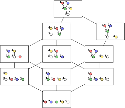
Figure 1: An interval in the poset $\Pi_{\operatorname{NAP}}(\{1,2,3,4,5\})$.

A poset $P$ is called totally semi-modular if for all $x,y\in P$, if there is $z$ that is covered by both $x$ and $y$, then there is $w$ which covers both $x$ and $y$.

Proposition 6.3

The intervals in $\Pi_{\operatorname{NAP}}(n)$ are totally semi-modular lattices.

• Proof. By relation (4) and Prop. 6.1, it is enough to prove the proposition for an interval of the form $[t,\widehat{1}]_{s}$. Let $x,y$ be two sub-rooted trees of $t$. Assume $x$ and $y$ cover a sub-rooted tree $z$. Hence $x$ is obtained from $z$ by removing a leaf $l_{x}$ and $y$ is obtained from $z$ by removing a leaf $l_{y}\not=l_{x}$. The sub-rooted tree $w$ obtained from $z$ by removing the leaves $l_{x}$ and $l_{y}$ covers both $x$ and $y$.  

Corollary 6.4

The posets $\Pi_{\operatorname{NAP}}(n)$ are Cohen-Macaulay.

• Proof. This follows from shellability, hence either from Prop. 6.3, as total semi-modularity implies CL-shellability [2], or from Prop. 6.2.  

Corollary 6.5

The operad $\operatorname{NAP}$ is Koszul.

• Proof. This follows from Vallette’s criterion Prop. 2.2 and the previous corollary.  

Proposition 6.6

In the $\operatorname{NAP}$ case, coinvariants are the same as isomorphism classes of posets between rooted trees.

• Proof. Coinvariants are given by unlabeled rooted trees. It is clear that if two rooted trees have the same underlying unlabeled rooted trees then their associated posets are isomorphic. Conversely, let $[\widehat{0},t]$ and $[\widehat{0},t^{\prime}]$ be two isomorphic posets. Then $[t,\widehat{1}]_{s}$ and $[t^{\prime},\widehat{1}]_{s}$ are isomorphic. This isomorphism induces a bijection between the labelling of the vertices of the two rooted trees and proves that $t$ and $t^{\prime}$ have the same underlying unlabeled rooted tree.  

This does not work for forests. The Hopf algebra $H_{\operatorname{NAP}}$ is not free on the coinvariants, as there are relations, given by the following proposition.

Proposition 6.7

Let $t=B(r,t_{1},\ldots,t_{k})$ be a rooted tree. The poset $[\widehat{0},t]$ is isomorphic to the product over $j\in\{1,\ldots,k\}$ of the posets $[\widehat{0},B(r,t_{j})]$.

• Proof. By Prop. 6.1 we prove the equivalent result for the interval $[t,\widehat{1}]_{s}$. Any sub-rooted tree $u$ of $t$ writes $u=B(r,u_{1},\ldots,u_{k})$, where $u_{i}$ is a sub-rooted tree of $t_{i}$ or may be the empty tree. The isomorphism sends $u$ to the product of the rooted trees $B(r,u_{j})$.  

6.3 Isomorphism between $H_{\operatorname{NAP}}$ and the Hopf algebra of Connes and Kreimer

In [6], Connes and Kreimer build a commutative Hopf algebra $\mathcal{H}_{R}$ , polynomial on unlabeled rooted trees. We prove in this section that $H_{\operatorname{NAP}}$ is isomorphic to this Hopf algebra.

Proposition 6.8

The Hopf algebra $H_{\operatorname{NAP}}$ is a free commutative algebra on the unlabeled rooted trees of root-valence 1.

• Proof. According to [15, Theorem 6.4], the Hopf algebra $H_{\mathcal{P}}$ is a free commutative algebra on its set of indecomposable elements. But each poset $[\widehat{0},t]$ with $t$ of root-valence $1$ cannot be written as a product (because there is only one element covered by $\widehat{1}$), hence is indecomposable. Conversely, any other interval decomposes as a product of such intervals by Prop. 6.7.  

Lemma 6.9

The elements $\mathsf{F}_{[t]}$, where $t$ runs over the set of rooted trees, form a basis of the vector space $H_{\operatorname{NAP}}$.

• Proof. As $H_{\operatorname{NAP}}$ is a free algebra on the elements $\mathsf{F}_{[x]}$ where $x$ is an unlabeled rooted tree of root-valence one by Prop. 6.8, a vector space basis is given by products $\mathsf{F}_{[t_{1}]}\dots\mathsf{F}_{[t_{k}]}$, with $t_{i}=B(r,t^{\prime}_{i})$. By Prop. 6.7, there exists a unique rooted tree $t=B(r,t^{\prime}_{1},\dots,t^{\prime}_{k})$ such that $\prod_{i}[\widehat{0},t_{i}]\simeq[\widehat{0},t]$. This gives a bijection between forests of unlabeled rooted trees of root-valence one and unlabeled rooted trees. Therefore the elements $\mathsf{F}_{[t]}$ where $[t]$ are unlabeled rooted trees form a basis.  

The Hopf algebra of Connes et Kreimer $\mathcal{H}_{R}$ is the free commutative algebra on unlabeled rooted trees with the following coproduct

$$\Delta(t)=1\otimes t+t\otimes 1+\sum_{c}P^{c}(t)\otimes R^{c}(t),$$

where $c$ stands for all the admissible cuts, $P^{c}(t)$ is a forest and $R^{c}(t)$ is a rooted tree defined from an admissible cut $c$ (see [6]). The coproduct has an alternative definition given by induction

$$\Delta(B^{+}(t_{1},\ldots,t_{k}))=B^{+}(t_{1},\ldots,t_{k})\otimes 1+(\mathrm{id}\otimes B^{+})(\Delta(t_{1}\ldots t_{k})),$$

where $B^{+}(t_{1},\ldots,t_{k})=B(r,t_{1},\ldots,t_{k})$. This means that the linear map $B^{+}:\mathcal{H}_{R}\rightarrow\mathcal{H}_{R}$ is a $1$-cocycle in the complex computing the Hochschild cohomology of the coalgebra $\mathcal{H}_{R}$. Indeed, Connes and Kreimer prove that $\mathcal{H}_{R}$ is a solution to a universal problem in Hochschild cohomology.

Theorem 6.10 ([6])

The pair $(\mathcal{H}_{R},B^{+})$ is universal among commutative Hopf algebras $(\mathcal{H},L)$ satisfying

$$\Delta(L(x))=L(x)\otimes 1+(\mathrm{id}\otimes L)(\Delta(x)),\forall x\in H.$$ (10)

More precisely, given such a Hopf algebra there exists a unique morphism of Hopf algebras $\phi:\mathcal{H}_{R}\rightarrow\mathcal{H}$ such that $L\circ\phi=\phi\circ B^{+}$.

As a consequence of the universal property, the Hopf algebra of Connes and Kreimer is unique up to isomorphism. We use this criteria to prove that $H_{\operatorname{NAP}}$ is isomorphic to $\mathcal{H}_{R}$.

Theorem 6.11

The Hopf algebra $H_{\operatorname{NAP}}$ is isomorphic to the Hopf algebra $\mathcal{H}_{R}$ of Connes and Kreimer. The unique isomorphism compatible with the universal property sends $\mathsf{F}_{[B(r,t_{1},\ldots,t_{k})]}$ to the forest $t_{1}\ldots t_{k}$.

• Proof. Let us define a $1$-cocycle $L_{\operatorname{NAP}}$ on $H_{\operatorname{NAP}}$.

  By lemma 6.9, it is enough to define $L_{\operatorname{NAP}}$ as

  $$L_{\operatorname{NAP}}(\mathsf{F}_{[t]})=\mathsf{F}_{[B(r,t)]},$$

  for each rooted tree $t$.

  Let us prove that $L_{\operatorname{NAP}}$ satisfies equation (10). For any rooted tree $u$, let $\psi_{u}$ be the isomorphism from $[\widehat{0},u]$ to $[u,\widehat{1}]_{s}$. The coproduct is then given by

  $$\Delta(\mathsf{F}_{[u]})=\sum_{x\leq u}\mathsf{F}_{[x]}\otimes\mathsf{F}_{[\psi_{u}(x)]},$$

  where $x$ is a forest of rooted trees and $\psi_{u}(x)$ is a sub-rooted tree of $u$. Hence

  $$\Delta(\mathsf{F}_{[B(r,t)]})=\sum_{x\leq B(r,t)}\mathsf{F}_{[x]}\otimes\mathsf{F}_{[\psi_{B(r,t)}(x)]}\\ =\mathsf{F}_{[B(r,t)]}\otimes 1+\sum_{x\leq t}\mathsf{F}_{[x]}\otimes\mathsf{F}_{[\psi_{B(r,t)}(\tilde{x})]}.$$

  Indeed, since $t$ is the unique rooted tree covered by $B(r,t)$, any $\tilde{x}<B(r,t)$ is the forest obtained from a forest of rooted trees $x\leq t$ by adding the rooted tree with the single vertex $r$. As a consequence $\psi_{B(r,t)}(\tilde{x})=B(r,\psi_{t}(x))$. Hence $L$ satisfies equation (10).

Let $(\mathcal{H},L)$ be a commutative Hopf algebra satisfying relation (10). In order to build a morphism of Hopf algebras $\rho:H_{\operatorname{NAP}}\rightarrow\mathcal{H}$, it is enough to give its values on the rooted trees of root-valence $1$. But such a generator can be written $\mathsf{F}_{[B(r,t)]}=L_{\operatorname{NAP}}(\mathsf{F}_{[t]})$. Hence we define $\rho(\mathsf{F}_{[B(r,\emptyset)]})=1$ since the rooted tree with single vertex $r$ is the unit and by induction $\rho(\mathsf{F}_{[B(r,t)]})=L(\rho(\mathsf{F}_{[t]}))$ where $\mathsf{F}_{[t]}$ is a product of generators of degree less than $B(r,t)$. It is straightforward to check that $\rho$ is a morphism of Hopf algebras such that $L\circ\rho=\rho\circ L_{\operatorname{NAP}}$.

As a consequence, $H_{\operatorname{NAP}}$ is isomorphic to $\mathcal{H}_{R}$, and the isomorphism goes as follows: $\mathsf{F}_{[B(r,t_{1},\ldots,t_{k})]}$ is sent to the forest $t_{1}\ldots t_{k}$.  

Let us give examples for the coproduct $\Delta$ in the incidence Hopf algebra $H_{\operatorname{NAP}}$:

$$\Delta\mathsf{F}_{\big{[}\includegraphics[height=14.22636pt]{a1200.eps}\big{]}}=1\otimes\mathsf{F}_{\big{[}\includegraphics[height=14.22636pt]{a1200.eps}\big{]}}+2\,\mathsf{F}_{\big{[}\includegraphics[height=14.22636pt]{a10.eps}\big{]}}\otimes\mathsf{F}_{\big{[}\includegraphics[height=14.22636pt]{a110.eps}\big{]}}+\mathsf{F}_{\big{[}\includegraphics[height=14.22636pt]{a200.eps}\big{]}}\otimes\mathsf{F}_{\big{[}\includegraphics[height=14.22636pt]{a10.eps}\big{]}}+\mathsf{F}_{\big{[}\includegraphics[height=14.22636pt]{a1200.eps}\big{]}}\otimes 1,$$

$$\Delta\mathsf{F}_{\big{[}\includegraphics[height=14.22636pt]{a2100.eps}\big{]}}=1\otimes\mathsf{F}_{\big{[}\includegraphics[height=14.22636pt]{a2100.eps}\big{]}}+\mathsf{F}_{\big{[}\includegraphics[height=14.22636pt]{a10.eps}\big{]}}\otimes(\mathsf{F}_{\big{[}\includegraphics[height=14.22636pt]{a200.eps}\big{]}}+\mathsf{F}_{\big{[}\includegraphics[height=14.22636pt]{a110.eps}\big{]}})+(\mathsf{F}_{\big{[}\includegraphics[height=14.22636pt]{a10.eps}\big{]}}^{2}+\mathsf{F}_{\big{[}\includegraphics[height=14.22636pt]{a110.eps}\big{]}})\otimes\mathsf{F}_{\big{[}\includegraphics[height=14.22636pt]{a10.eps}\big{]}}+\mathsf{F}_{\big{[}\includegraphics[height=14.22636pt]{a2100.eps}\big{]}}\otimes 1,$$

and

$$\Delta\mathsf{F}_{\big{[}\includegraphics[height=14.22636pt]{a3000.eps}\big{]}}=1\otimes\mathsf{F}_{\big{[}\includegraphics[height=14.22636pt]{a3000.eps}\big{]}}+3\,\mathsf{F}_{\big{[}\includegraphics[height=14.22636pt]{a10.eps}\big{]}}\otimes\mathsf{F}_{\big{[}\includegraphics[height=14.22636pt]{a200.eps}\big{]}}+3\,\mathsf{F}_{\big{[}\includegraphics[height=14.22636pt]{a200.eps}\big{]}}\otimes\mathsf{F}_{\big{[}\includegraphics[height=14.22636pt]{a10.eps}\big{]}}+\mathsf{F}_{\big{[}\includegraphics[height=14.22636pt]{a3000.eps}\big{]}}\otimes 1,$$

where we have used that ${\mathsf{F}_{\left[\includegraphics[height=5.69054pt]{a0small.eps}\right]}}$ is the unit $1$. The last example also follows from the equality (see Prop. 6.7)

$$\mathsf{F}_{\big{[}\includegraphics[height=14.22636pt]{a3000.eps}\big{]}}=\mathsf{F}_{\big{[}\includegraphics[height=14.22636pt]{a10.eps}\big{]}}^{3}.$$

The similar coproducts in the Hopf algebra $\mathbb{Q}[G_{\operatorname{NAP}}]$ are

$$\Delta\mathsf{G}_{\includegraphics[height=14.22636pt]{a1200.eps}}=1\otimes\mathsf{G}_{\includegraphics[height=14.22636pt]{a1200.eps}}+\mathsf{G}_{\includegraphics[height=14.22636pt]{a10.eps}}\otimes\mathsf{G}_{\includegraphics[height=14.22636pt]{a110.eps}}+\mathsf{G}_{\includegraphics[height=14.22636pt]{a200.eps}}\otimes\mathsf{G}_{\includegraphics[height=14.22636pt]{a10.eps}}+\mathsf{G}_{\includegraphics[height=14.22636pt]{a1200.eps}}\otimes 1,$$

$$\Delta\mathsf{G}_{\includegraphics[height=14.22636pt]{a2100.eps}}=1\otimes\mathsf{G}_{\includegraphics[height=14.22636pt]{a2100.eps}}+\mathsf{G}_{\includegraphics[height=14.22636pt]{a10.eps}}\otimes(2\,\mathsf{G}_{\includegraphics[height=14.22636pt]{a200.eps}}+\mathsf{G}_{\includegraphics[height=14.22636pt]{a110.eps}})+(\mathsf{G}_{\includegraphics[height=14.22636pt]{a10.eps}}^{2}+\mathsf{G}_{\includegraphics[height=14.22636pt]{a110.eps}})\otimes\mathsf{G}_{\includegraphics[height=14.22636pt]{a10.eps}}+\mathsf{G}_{\includegraphics[height=14.22636pt]{a2100.eps}}\otimes 1,$$

and

$$\Delta\mathsf{G}_{\includegraphics[height=14.22636pt]{a3000.eps}}=1\otimes\mathsf{G}_{\includegraphics[height=14.22636pt]{a3000.eps}}+\mathsf{G}_{\includegraphics[height=14.22636pt]{a10.eps}}\otimes\mathsf{G}_{\includegraphics[height=14.22636pt]{a200.eps}}+\mathsf{G}_{\includegraphics[height=14.22636pt]{a200.eps}}\otimes\mathsf{G}_{\includegraphics[height=14.22636pt]{a10.eps}}+\mathsf{G}_{\includegraphics[height=14.22636pt]{a3000.eps}}\otimes 1,$$

where we have also used that ${\mathsf{G}_{\includegraphics[height=5.69054pt]{a0small.eps}}}$ is the unit $1$.

6.4 Examples of elements of the group $G_{\operatorname{NAP}}$

The group $G_{\operatorname{NAP}}$ can be considered as a group of formal power series indexed by the set of unlabeled rooted trees. In this section, we give a criterion for an element of $G_{\operatorname{NAP}}$ to be in $\operatorname{Spec}H_{\operatorname{NAP}}$, then describe several examples of elements of $G_{\operatorname{NAP}}$ and compute their inverses.

Let us first describe explicitly the image of $\operatorname{Spec}H_{\operatorname{NAP}}$ in $G_{\operatorname{NAP}}$.

Lemma 6.12

A series $f=\sum_{t}\mathsf{G}_{t}(f)t$ in $G_{\operatorname{NAP}}$ is in the subgroup $\operatorname{Spec}H_{\operatorname{NAP}}$ if and only if for each tree $t=B(r,t_{1},\dots,t_{k})$, one has

$$\operatorname{\#Aut}(B(r,t_{1},\dots,t_{k}))\mathsf{G}_{B(r,t_{1},\dots,t_{k})}(f)=\prod_{i=1}^{k}\operatorname{\#Aut}(B(r,t_{i}))\mathsf{G}_{B(r,t_{i})}(f).$$

• Proof. Indeed, if the series $f$ is the image of an element $f^{\prime}$ in $\operatorname{Spec}H_{\operatorname{NAP}}$, then one has $\mathsf{G}_{t}(f)=\mathsf{F}_{[t]}(f^{\prime})/\operatorname{\#Aut}(t)$, and the multiplicative behavior follows from Prop. 6.7. Conversely, if the multiplicativity property holds, one can build a unique element $f^{\prime}$ in $\operatorname{Spec}H_{\operatorname{NAP}}$ that maps to $f$.  

The first example is in fact an element of the subgroup $\operatorname{Spec}H_{\operatorname{NAP}}$ and we can therefore deduce its inverse by first computing the Möbius numbers of the maximal intervals in $\Pi_{\operatorname{NAP}}(n)$.

Proposition 6.13

Let $t$ be a rooted tree. If $t$ is a corolla with $n+1$ vertices, then $\mu(\widehat{0},t)=(-1)^{n}$. If not, then $\mu(\widehat{0},t)=0$.

• Proof. We compute the Möbius number of the poset $[t,\widehat{1}]_{s}$. If $t$ is the rooted tree $t_{2}$ with only two vertices then the Möbius number of the interval $[t,\widehat{1}]_{s}$ is clearly $-1$. Hence the Prop. 6.7 yields the result for the corollas. If the valence of the root of $t$ is one then $\widehat{1}$ covers a unique rooted tree which is $t_{2}$. If $t$ has at least $3$ vertices, then $t_{2}$ is different from $t$ and the Möbius number of the interval $[t,1]_{s}$ is $0$. If the valence of the root of $t$ is greater than 2 and $t$ is not a corolla, then in the decomposition of $t=B(r,t_{1},\ldots,t_{k})$, there exists $t_{i}$ having at least two vertices. The rooted tree $B(r,t_{i})$ has root-valence 1 and has at least $3$ vertices so its Möbius number is 0. We conclude with Prop. 6.7.  

We now deduce from this computation an identity in the group $G_{\operatorname{NAP}}$.

Consider the series where each rooted tree has weight the inverse of the order of its automorphism group:

$$\mathtt{Z}=\includegraphics[height=14.22636pt]{a0.eps}+\includegraphics[height=14.22636pt]{a10.eps}+\frac{1}{2}\,\includegraphics[height=14.22636pt]{a200.eps}+\includegraphics[height=14.22636pt]{a110.eps}+\frac{1}{6}\,\includegraphics[height=14.22636pt]{a3000.eps}+\frac{1}{2}\,\includegraphics[height=14.22636pt]{a1200.eps}+\includegraphics[height=14.22636pt]{a2100.eps}+\includegraphics[height=14.22636pt]{a1110.eps}+\dots$$

By Lemma 6.12, this belongs to the image of $\operatorname{Spec}H_{\operatorname{NAP}}$ and should be called the Zeta function, following the standard notation in algebraic combinatorics of posets [14, 16].

By the general result Prop. 3.2, its inverse in the group $\operatorname{Spec}H_{\operatorname{NAP}}$ is known to be the generating series for Möbius numbers.

Hence by the computation of Möbius numbers done in Prop. 6.13 and the inclusion of $\operatorname{Spec}H_{\operatorname{NAP}}$ in $G_{\operatorname{NAP}}$ obtained in Th. 5.4, the inverse of $\mathtt{Z}$ in the group $G_{\operatorname{NAP}}$ is the similar sum $\mathtt{M}$ restricted on corollas and with additional signs:

$$\mathtt{M}=\includegraphics[height=14.22636pt]{a0.eps}-\includegraphics[height=14.22636pt]{a10.eps}+\frac{1}{2}\includegraphics[height=14.22636pt]{a200.eps}-\frac{1}{6}\includegraphics[height=14.22636pt]{a3000.eps}+\frac{1}{24}\includegraphics[height=14.22636pt]{a40000.eps}+\dots$$

We now give some other examples of elements of $G_{\operatorname{NAP}}$.

Let us introduce the sum of all corollas in $G_{\operatorname{NAP}}$:

$$\mathtt{C}=\includegraphics[height=14.22636pt]{a0.eps}+\includegraphics[height=14.22636pt]{a10.eps}+\includegraphics[height=14.22636pt]{a200.eps}+\includegraphics[height=14.22636pt]{a3000.eps}+\includegraphics[height=14.22636pt]{a40000.eps}+\dots$$

and the alternating sum of linear trees:

$$\mathtt{L}=\includegraphics[height=14.22636pt]{a0.eps}-\includegraphics[height=14.22636pt]{a10.eps}+\includegraphics[height=14.22636pt]{a110.eps}-\includegraphics[height=14.22636pt]{a1110.eps}+\includegraphics[height=14.22636pt]{a11110.eps}-\dots$$

The series $\mathtt{C}$ satisfies the simple functional equation

$$\mathtt{C}=\includegraphics[height=14.22636pt]{a0.eps}+\mathtt{C}\triangleleft\includegraphics[height=14.22636pt]{a0.eps},$$ (11)

where $\triangleleft$ is the $\operatorname{NAP}$ product on rooted trees.

Theorem 6.14

In the group $G_{\operatorname{NAP}}$, one has $\mathtt{C}=\mathtt{L}^{-1}$.

• Proof. From the functional equation (11) for $\mathtt{C}$, one gets

  $$\includegraphics[height=14.22636pt]{a0.eps}=\mathtt{C}^{-1}+\includegraphics[height=14.22636pt]{a0.eps}\triangleleft\mathtt{C}^{-1},$$

  by product by $\mathtt{C}^{-1}$ on the right, since one has in $G_{\operatorname{NAP}}$ the relation $(\mathtt{C}\triangleleft\mathtt{D})\times\mathtt{E}=(\mathtt{C}\times\mathtt{E})\triangleleft(\mathtt{D}\times\mathtt{E})$. But the unique solution to this equation is easily seen to be $\mathtt{L}$.  

One can see from Lemma 6.12 that the series $\mathtt{C}$ and $\mathtt{L}$ do not belong to the subgroup $\operatorname{Spec}H_{\operatorname{NAP}}$, as the coefficients $\operatorname{\#Aut}(t)\mathsf{G}_{t}$ do not have the necessary multiplicativity property. For instance, the coefficients of corollas vanish in $\mathtt{L}$, but the coefficient of the tree does not.

6.5 Morphisms from $G_{\operatorname{NAP}}$ to usual power series

There are two morphisms from the group $G_{\operatorname{NAP}}$ to the multiplicative group of formal power series in one variable $x$. Either one can project on corollas:

$$\sum_{t}\mathsf{G}_{t}\,t\mapsto\sum_{n\geq 0}\mathsf{G}_{c_{n}}x^{n},$$

where $c_{n}$ is the corolla with $n$ leaves, or project on linear trees:

$$\sum_{t}\mathsf{G}_{t}\,t\mapsto\sum_{n\geq 0}\mathsf{G}_{\ell_{n}}x^{n},$$

where $\ell_{n}$ is the linear tree with $n+1$ vertices.

Recall that the Hopf algebra of functions on the multiplicative group of formal power series

$$1+\sum_{n\geq 1}M_{n}x^{n}$$

is the free commutative algebra with one generator $M_{n}$ in each degree $n\geq 1$ and coproduct

$$\Delta M_{n}=\sum_{i=0}^{n}M_{i}\otimes M_{n-i},$$

with the convention that $M_{0}=1$.

It is indeed easy to check that corollas and linear trees are closed on the coproduct and that the coproduct is the same as in the multiplicative group.

In the case of linear trees, the induced morphism from $\operatorname{Spec}H_{\operatorname{NAP}}$ to the multiplicative group of formal power series is again a projection. This means that it defines a Hopf subalgebra of $H_{\operatorname{NAP}}$, corresponding to the ladder Hopf subalgebra in $\mathcal{H}_{R}$.

The reader may want to check that the image of the inverse is the inverse of the image, in the examples $\mathtt{C}$, $\mathtt{L}$, $\mathtt{Z}$ and $\mathtt{M}$ given above.

There is a morphism from the group $G_{\operatorname{NAP}}$ to the group of formal power series in one variable $x$ for composition given by the sum of the coefficients of all rooted trees of same degree:

$$\sum_{t}\mathsf{G}_{t}\,t\mapsto\sum_{n\geq 1}\left(\sum_{t\in\operatorname{NAP}(n)_{\mathfrak{S}_{n}}}\mathsf{G}_{t}\right)\,x^{n}.$$

This comes from the morphism of operads from $\operatorname{NAP}$ to the Commutative operad $\operatorname{Comm}$ which sends every element of $\operatorname{NAP}(n)$ to the unique element of $\operatorname{Comm}(n)$.

One can easily check that the images of the series $\mathtt{C}$ and $\mathtt{L}$ are inverses for composition. For the images of the series $\mathtt{Z}$ and $\mathtt{M}$, this is less obvious. This implies that the image of $\mathtt{Z}$ is

$$\sum_{n\geq 1}n^{n-1}\frac{x^{n}}{n!},$$

which is the functional inverse of $x\exp(-x)$. This is related to the Lambert W function [7], the inverse of $x\exp(x)$.

It is easy to see that the induced morphism from $\operatorname{Spec}H_{\operatorname{NAP}}$ to the composition group of formal power series is again a projection, hence defines a Hopf subalgebra of $H_{\operatorname{NAP}}$. This Hopf algebra is isomorphic to the Faà di Bruno Hopf algebra as pointed out in §5. The generators of the subalgebra $\mathbb{Q}[G_{\operatorname{Comm}}]$ in $\mathbb{Q}[G_{\operatorname{NAP}}]$ are

$$\sum_{t\in\operatorname{NAP}(n)_{\mathfrak{S}_{n}}}\mathsf{G}_{t},$$

for $n\geq 2$. Hence the generators of the subalgebra in $H_{\operatorname{NAP}}$ are

$$\sum_{t\in\operatorname{NAP}(n)_{\mathfrak{S}_{n}}}\frac{1}{\operatorname{\#Aut}(t)}\mathsf{F}_{[t]},$$

for $n\geq 2$.

Let us give explicitly the first generators of this Hopf subalgebra of $H_{\operatorname{NAP}}$:

$$\Gamma_{1}= \mathsf{F}_{\big{[}\includegraphics[height=14.22636pt]{a10.eps}\big{]}},$$

$$\Gamma_{2}= \mathsf{F}_{\big{[}\includegraphics[height=14.22636pt]{a110.eps}\big{]}}+\frac{1}{2}\mathsf{F}_{\big{[}\includegraphics[height=14.22636pt]{a200.eps}\big{]}}=\mathsf{F}_{\big{[}\includegraphics[height=14.22636pt]{a110.eps}\big{]}}+\frac{1}{2}\mathsf{F}_{\big{[}\includegraphics[height=14.22636pt]{a10.eps}\big{]}}^{2},$$

$$\Gamma_{3}= \mathsf{F}_{\big{[}\includegraphics[height=14.22636pt]{a1110.eps}\big{]}}+\frac{1}{2}\mathsf{F}_{\big{[}\includegraphics[height=14.22636pt]{a1200.eps}\big{]}}+\mathsf{F}_{\big{[}\includegraphics[height=14.22636pt]{a2100.eps}\big{]}}+\frac{1}{6}\mathsf{F}_{\big{[}\includegraphics[height=14.22636pt]{a3000.eps}\big{]}}=\mathsf{F}_{\big{[}\includegraphics[height=14.22636pt]{a1110.eps}\big{]}}+\frac{1}{2}\mathsf{F}_{\big{[}\includegraphics[height=14.22636pt]{a1200.eps}\big{]}}+\mathsf{F}_{\big{[}\includegraphics[height=14.22636pt]{a110.eps}\big{]}}\mathsf{F}_{\big{[}\includegraphics[height=14.22636pt]{a10.eps}\big{]}}+\frac{1}{6}\mathsf{F}_{\big{[}\includegraphics[height=14.22636pt]{a10.eps}\big{]}}^{3},$$

where we have used the multiplicative property of the $\mathsf{F}$ functions to get from sums over all rooted trees to polynomials in rooted trees of root-valence $1$.

By mapping these elements to the Connes-Kreimer algebra $\mathcal{H}_{R}$ by the isomorphism of Theorem 6.11, one can see that this Hopf subalgebra is different from the Connes-Moscovici subalgebra and also from the other Hopf subalgebras of $\mathcal{H}_{R}$ introduced recently by Foissy [8].

References

• [1] G. Birkhoff. Lattice theory. Third edition. American Mathematical Society Colloquium Publications, Vol. XXV. American Mathematical Society, Providence, R.I., 1967.
• [2] A. Björner and M. Wachs. On lexicographically shellable posets. Trans. Amer. Math. Soc., 277(1):323–341, 1983.
• [3] F. Chapoton. Rooted trees and an exponential-like series. arXiv:math.QA/0209104.
• [4] F. Chapoton and M. Livernet. Pre-Lie algebras and the rooted trees operad. Internat. Math. Res. Notices, 8:395–408, 2001.
• [5] F. Chapoton and B. Vallette. Pointed and multi-pointed partitions of type $A$ and $B$. J. Algebraic Combin., 23(4):295–316, 2006.
• [6] A. Connes and D. Kreimer. Hopf algebras, renormalization and noncomutative geometry. Comm. Math. Phys., 199:203–242, 1998.
• [7] R. M. Corless, G. H. Gonnet, D. E. G. Hare, D. J. Jeffrey, and D. E. Knuth. On the Lambert $W$ function. Adv. Comput. Math., 5(4):329–359, 1996.
• [8] L. Foissy. Faà di Bruno subalgebras of the Hopf algebras of planar trees. arXiv:0707.1204, 2007.
• [9] A. Joyal. Foncteurs analytiques et espèces de structures. In Combinatoire énumérative (Montreal, Que., 1985/Quebec, Que., 1985), volume 1234 of Lecture Notes in Math., pages 126–159. Springer, Berlin, 1986.
• [10] M. Kapranov and Yu. Manin. Modules and Morita theorem for operads. Amer. J. Math., 123(5):811–838, 2001.
• [11] M. Livernet. A rigidity theorem for pre-Lie algebras. J. Pure Appl. Algebra, 207(1):1–18, 2006.
• [12] P. McNamara. EL-labelings, supersolvability and 0-Hecke algebra actions on posets. J. Combin. Theory Ser. A, 101(1):69–89, 2003.
• [13] M. Méndez and J. Yang. Möbius species. Adv. Math., 85(1):83–128, 1991.
• [14] G.-C. Rota. On the foundations of combinatorial theory. I. Theory of Möbius functions. Z. Wahrscheinlichkeitstheorie und Verw. Gebiete, 2:340–368 (1964), 1964.
• [15] W. R. Schmitt. Incidence Hopf algebras. J. Pure Appl. Algebra, 96(3):299–330, 1994.
• [16] R. P. Stanley. Enumerative combinatorics. Vol. 1, volume 49 of Cambridge Studies in Advanced Mathematics. Cambridge University Press, Cambridge, 1997. With a foreword by Gian-Carlo Rota, Corrected reprint of the 1986 original.
• [17] B. Vallette. Homology of generalized partition posets. J. Pure Appl. Algebra, 208(2):699–725, 2007.
• [18] P. van der Laan. Operads. Hopf algebras and coloured Koszul duality. PhD thesis, Universiteit Utrecht, 2004.
Muriel Livernet
Laboratoire Analyse,
Géométrie et Applications,
UMR 7539 du CNRS,
Institut Galilée,
Université Paris Nord
Avenue Jean Baptiste Clément,
93430 VILLETANEUSE.
livernet@math.univ-paris13.fr
Frédéric Chapoton
Université de Lyon ;
Université Lyon 1 ;
Institut Camille Jordan CNRS UMR 5208 ;
43, boulevard du 11 novembre 1918,
F-69622 Villeurbanne Cedex.
fchapoton@math.univ-lyon1.fr