Abstract

Effective low energy models arising in the context of D-brane configurations with Standard Model (SM) gauge symmetry extended by several gauged abelian factors are discussed. The models are classified according to their hypercharge embeddings consistent with the SM spectrum hypercharge assignment. Particular cases are analyzed according to their perspectives and viability as low energy effective field theory candidates. The resulting string scale is determined by means of a two-loop renormalization group calculation. Their implications in Yukawa couplings, neutrinos and flavor changing processes are also presented.

July 2007

1 Introduction

The revelation of the higher dimensional objects [1], called D-branes, has revived the interest on model building in the context of string theory. As a consequence, during the last decade, numerous painstaking efforts have been devoted to the study of possible D-brane realizations of the Standard Model and the higher gauge symmetries containing it.

Model building in string theory has shown that there is no a priori obvious recipe to obtain the SM from the first principles of the theory. In recent attempts, various groups [3]-[11] started mainly a bottom-up approach delving into the string vacua, aiming to systematically classify all possible D-brane configurations, seeking an acceptable effective low energy theory which reproduces the success of the Standard Model. It is anticipated that, such a construction would determine the arbitrary parameters of the Standard Model, while new phenomena could be predicted and eventually tested in future experiments.

In the present work, we elaborate on low energy implications of a particular class of D-brane models [4]-[11] with Standard Model gauge symmetry and Split Supersymmetric spectrum [12]. The implementation of Split Supersymmetry in the D-brane constructions under consideration, is justified for the following two reasons: First, it was shown that the realization of Split Susy is a viable possibility in certain D-brane constructions [14]. Second, intermediate and high string scale D-brane models previously abandoned because of phenomenological drawbacks related to hierarchy problems, rapid proton decay etc, in the context of Split Supersymmetry offer fascinating new possibilities since there exist now convincing arguments concerning the hierarchy issues. Besides, the renormalization group flow of the gauge and Yukawa couplings as well as low energy measurable physical quantities dependent on them, change substantially. In view of these interesting novelties, in a previous work [6], a classification of the various D-brane derived models with Split Supersymmetric spectrum and Standard Model gauge symmetry extended by $U(1)$ factors was attempted. All possible configurations with $P=1,2,3$ abelian branes were considered and the different hypercharge embeddings compatible with the SM particle spectrum were found. In all viable cases, a one-loop RG analysis was used to calculate the string scale $M_{S}$, while the fermion mass relations of the third generation, the gaugino masses and the lifetime of the gluino were examined. Here, we will pursue a further investigation, addressing more phenomenological issues and deriving possible constraints on the Split Supersymmetry breaking scale $\tilde{m}$ and other so far undetermined parameters. We will extend our previous analysis, and work out in detail the predictions for the string scale using renormalization group equations at two–loop order. We note however, that the determination of the string scale is more intricate than in ordinary Grand Unified models. The reason is that in D-brane constructions, gauge coupling unification at the string scale does not occur since the volume of the internal space is involved between gauge and string couplings; thus, the actual values of the SM gauge coupling constants may differ at $M_{S}$. This arbitrariness looks rather daunting, however, certain internal volume relations could allow for partial unification. In order to reduce the number of free parameters and obtain definite predictions, we mainly concentrate on cases where certain relations are assumed to connect the gauge couplings at the string scale. Particular attention is also given to models where the non-abelian gauge couplings have a common value at $M_{S}$. Next, in each case of the models under consideration, we determine the range of the Split Supersymmetric scale which is compatible with the chosen gauge coupling conditions. We further discuss the Yukawa potential and other low energy predictions which are crucial for the viability of the models. In particular, we examine the conditions under which exotic processes like the lepton flavor violating decay $\mu\rightarrow e\gamma$ can be detected in future experiments, we discuss suggested mechanisms predicting a sufficiently heavy mass for the right-handed neutrino and check the existence of exotic matter like leptoquarks, whose appearance is also possible in the low energy spectrum of these models.

The paper is organized as follows: In the next section, we summarize the salient features of the D-brane configurations and determine the hypercharge embeddings leading to Standard Model particle spectrum. In section 3 we present in some detail selected cases of low energy effective models, while in section 4 we calculate the string scale and explore its correlation with the Split Supersymmetric scale by means of a two-loop renormalization group analysis. In section 5 we analyze the effects of exotic states. In section 6 we discuss the observability conditions for rare flavor violation like $\mu\rightarrow e\gamma$. Finally, in section 7 we present our conclusions.

2 D-brane configurations and Split Supersymmetry

The embedding of the Standard Model in a D-brane configuration as well as some implications in low energy phenomenology and the magnitude of the string scale have been explored in several works  [4, 5, 6, 7, 8]. The same problem in the context of intersecting D-branes, has also been extensively discussed [9, 10].

The resulting field theory model involves the SM non-abelian gauge symmetry extended by several $U(1)$ factors, a linear combination of which defines the hypercharge. A systematic bottom-up investigation of all possible configurations for the SM gauge symmetry with two abelian branes was presented in [7]. Here, as in [8], we assume the existence of at most three extra $U(1)$ abelian branes, thus, the full gauge group is

$$G={U(3)}_{C}\times{U(2)}_{L}\times{U(1)}^{P},\;P=1,2,3\,\cdot$$ (1)

Since $U(n)\sim{SU(n)}\times{U(1)}$, the final symmetry is

$$G={SU(3)}_{C}\times{SU(2)}_{L}\times{U(1)}^{P+2},\;P=1,2,3$$ (2)

while the SM fermions and Higgs fields carry additional quantum numbers under the extra $U(1)$’s.

Given that strings attached to various D-brane stacks represent the SM matter fields, the hypercharge generator is in general, a linear combination of all possible $U(1)$ factors. If we define the anomaly free linear combination of these $U(1)$’s to be

$$Y=k_{3}Q_{3}+k_{2}Q_{2}+\sum_{i=1}^{3}k_{i}^{\prime}Q_{i}^{\prime}$$

the most general hypercharge gauge coupling condition can be written as

$$\frac{1}{g_{Y}^{2}}=\frac{6k_{3}^{2}}{g_{3}^{2}}+\frac{4k_{2}^{2}}{g_{2}^{2}}+2\sum_{i=1}^{P}\frac{{k^{\prime}_{i}}^{2}}{{g^{\prime}_{i}}^{2}}\ \cdot$$ (3)

For a given hypercharge embedding, the $k_{i}^{\prime}$’s can be determined and equation (3) relates the weak angle $\sin^{2}\theta_{W}=({1+k_{Y}})^{-1}$ ( $k_{Y}=\frac{\alpha_{2}}{\alpha_{Y}}$, $\alpha_{i}\equiv g_{i}^{2}/4\pi$), with the gauge coupling ratios at the string scale $M_{S}$. Since in D-brane scenarios the gauge couplings do not necessarily attain a common value at the string (brane) scale $M_{S}$, the ratios $\alpha_{2}/\alpha_{3}$, $\alpha_{2}/\alpha_{i}^{\prime}$ differ from unity there. In a previous analysis, various relations between the gauge couplings were considered and a systematic investigation of the magnitude of the string scale and the split SUSY breaking mass scale was presented [8]. Here, in order to reduce the arbitrary parameters and come up with definite predictions, we assume the existence of relations between the gauge couplings at $M_{S}$, while we pay particular attention to the interesting case $\alpha_{2}=\alpha_{3}$ at $M_{S}$. If we accept that $m\leq P$ $U(1)$ branes are aligned with the $U(3)$ stack and the remaining $P-m$ abelian branes are aligned with the $U(2)$ set, $k_{Y}$ becomes

$$k_{Y} \equiv \frac{\alpha_{2}}{\alpha_{Y}}\;=\;n_{1}\,\xi+n_{2}$$ (4)

where

$$n_{1}={6k_{3}^{2}}+2\sum_{i=1}^{m}{k_{i}^{\prime}}^{2}, n_{2}=4k_{2}^{2}+2\sum_{i=m+1}^{P}{k_{i}^{\prime}}^{2},$$ (5)

and $\xi$ is the ratio of the non-abelian gauge couplings ${\alpha_{2}}/{\alpha_{3}}$.

To obtain the fermion and Higgs spectrum of a given brane configuration, we note that each state corresponds to an open string stretched between pairs of brane stacks or to a string with both ends attached to the same brane stack. Taking all possible arrangements of the SM particle spectrum represented by the various strings attached between the $U(3)$, $U(2)$ and extra $U(1)_{i}$ brane sets, we end up with the admissible brane configurations. Some particular arrangements are shown in figure 1. For each particular configuration, the coefficients $k_{2,3},k_{i}^{\prime}$ are determined by the requirement that the SM particle spectrum acquires the correct hypercharge.

To proceed further, we recall here the results obtained for brane setups that include up to three abelian branes. The admissible solutions for the $U(3)\times U(2)\times U(1)$ case setup have been explored in  [14] and the $k_{i}$ distinctive solutions are presented in the first two lines of Table 1. For the $U(3)\times U(2)\times U(1)^{2}$ configuration [4, 5, 7], we assign the quantum numbers of the SM particles $Q(3,2;+1,\epsilon_{1},0,0)$, $d^{c}(\bar{3},1;-1,0,\epsilon_{2},0)$, $u^{c}(\bar{3},1;-1,0,0,-\epsilon_{3})$, $L(1,2;0,\epsilon_{4},0,\epsilon_{5})$ and $e^{c}(1,1;0,0,\epsilon_{6},\epsilon_{7})$, where $\epsilon_{i}=\pm 1$. A similar assignment can be written for the $P=3$ case too. Solving the corresponding hypercharge assignment equations [6, 8], we find that the hypercharge can be expressed in terms of $k_{2}^{\prime}=x$ which remains undetermined, as

$$Y = (2/3-x)\,Q_{3}+(1/2-x)\,Q_{2}+(1-x)\,Q_{1}^{\prime}+x\,Q_{2}^{\prime}+\delta_{N3}\,x\,Q_{3}^{\prime}\ \cdot$$ (6)

Choosing appropriate values for $x$ so that the corresponding boson remains massless at $M_{S}$, the simplest solutions for the three different brane configurations are shown in Table 1. For future use, the values of the coefficients $n_{1},n_{2}$ appearing in (5) for all possible $U(3)$ and/or $U(2)$ alignments of the $U(1)$ branes are also included in the last column of the same Table.

$P$		$|k_{3}|$	$|k_{2}|$	$|k_{1}^{\prime}|$	$|k_{2}^{\prime}|$	$|k_{3}^{\prime}|$	$(n_{1},n_{2})$
	$a_{1}$	$\frac{1}{3}$	$\frac{1}{2}$	$0$	$-$	$-$	$(\frac{2}{3},1)$
$1$	$b_{1}$	$\frac{1}{6}$	$0$	$\frac{1}{2}$	$-$	$-$	$(\frac{2}{3},0);(\frac{1}{6},\frac{1}{2})$
	$a_{2}$	$\frac{1}{6}$	$0$	$\frac{1}{2}$	$\frac{1}{2}$	$-$	$(\frac{1}{6},1);(\frac{7}{6},0);(\frac{2}{3},\frac{1}{2})$
$2$	$b_{2}$	$\frac{2}{3}$	$\frac{1}{2}$	$1$	$0$	$-$	$(\frac{8}{3},3);(\frac{14}{3},1)$
	$c_{2}$	$\frac{1}{3}$	$\frac{1}{2}$	$0$	$1$	$-$	$(\frac{2}{3},3);(\frac{8}{3},1)$
	$a_{3}$	$\frac{1}{6}$	$0$	$\frac{1}{2}$	$\frac{1}{2}$	$\frac{1}{2}$	$(\frac{1}{6},\frac{3}{2});(\frac{2}{3},1);(\frac{5}{3},0);(\frac{7}{6},\frac{1}{2})$
$3$	$b_{3}$	$\frac{1}{3}$	$\frac{1}{2}$	$0$	$1$	$1$	$(\frac{2}{3},5);(\frac{14}{3},1);(\frac{8}{3},3)$
	$c_{3}$	$\frac{2}{3}$	$\frac{1}{2}$	$1$	$0$	$0$	$(\frac{8}{3},3);(\frac{14}{3},1)$

Table 1: Simplest hypercharge embeddings for the $P=1,2,3$ brane configurations. The last column shows the $(n_{1},n_{2})$-values of (5) for the various possible alignments of the $U(1)$-branes with respect to $U(3)$ and $U(2)$ brane-stack orientations.

Figure 1: Selected Standard Model configurations with one, two and three abelian branes $P=1,2,3$.

3 Low energy effective models of particular embeddings

In the previous section we saw that the SM spectrum can be successfully accommodated in D-brane setups with gauge symmetry of the form $U(3)\times U(2)\times U(1)^{P}$, $P=1,2,3$, and made a complete classification of models for the various hypercharge embeddings which imply a realistic particle content. In this section, we will present the particular embeddings in more detail, and work out the Yukawa couplings and other phenomenologically interesting features.

In a previous work [8], we presented an analysis dealing with the implications of Split Supersymmetry on the string scale, first considering models that arise in parallel brane scenarios where the $U(1)$ branes are superposed with the $U(2)$ or $U(3)$ brane stacks. Varying the Split Susy scale in a wide range, we examined the evolution of the gauge couplings and found three distinct classes of models with respect to the string scale. The Split Supersymmetry breaking scale $\tilde{m}$, can in principle be much larger than the electroweak scale and, as a consequence, squarks and sleptons can obtain large masses of order $\tilde{m}$, while the corresponding fermionic degrees as well as gauginos and higgsinos, remain light. This splitting of the spectrum is made possible only when the dominant source of supersymmetry breaking preserves an R-symmetry which protects fermionic degrees from obtaining masses at the scale $\tilde{m}$.

Assuming that above $\tilde{m}$ only the MSSM spectrum exists, while below $\tilde{m}$ we only have SM fermions, gauginos, higgsinos and one linear combination of the scalar Higgs doublets, the one-loop RGE expression for the string scale is given by

$$M_{S} = M_{Z}\,\left(\frac{\tilde{m}}{M_{Z}}\right)^{a}e^{b}$$ (7)

where, the parameters $a,b$ depend on the beta function coefficients, the values of the gauge couplings at $M_{Z}$ and the model dependent constants $n_{1},n_{2}$ given in (5). After substituting the beta functions, these constants are given by

$$a = \frac{21-12n_{1}-13n_{2}}{6(11+3n_{1}-n_{2})}$$

$$b = \frac{2\pi}{11+3n_{1}-n_{2}}\left(\frac{1}{\alpha_{Y}}-\frac{n_{2}}{\alpha_{2}}-\frac{n_{1}}{\alpha_{3}}\right)\cdot$$

The above one-loop formula is sufficient to produce some qualitative results. Thus, one class of models that arises in the configurations with $P=1$ and $P=3$ abelian branes, predicts a string scale of the order of the SUSY GUT scale $M_{S}\sim 10^{16}$ GeV; interestingly enough, these models also imply that the non-abelian gauge couplings unify ($\alpha_{2}=\alpha_{3}$) at $M_{S}$.

In the case of the configuration with only one abelian brane, the up or down right handed quarks arise when both endpoints of an open string are attached to the color stack. In this case, the terms $Qu^{c}$ or $Qd^{c}$ carry a non-zero $U(1)_{C}$ charge while a typical SM Higgs field is not charged under $U(1)_{C}$. Therefore, the corresponding tree-level Yukawa term is not allowed and the quark fields remain massless. It is worth noting that, as shown by one-loop renormalization group analysis [8], $\tilde{m}$, at least in its minimal SM content, is fixed at a relatively small scale $\sim 6$ TeV. The corresponding –with respect to the $M_{S}\sim 10^{16}$ GeV prediction– $P=3$ case, is free from these shortcomings, consequently, in what follows, we are going to further elaborate on some interesting low energy implications of this setup.

Another category of brane configurations was found in a particular –with respect to the $U(1)$ alignments– case of the $P=2$ abelian branes. This model corresponds to a specific $U(1)$ brane orientation and predicts an intermediate string scale $M_{S}\sim 10^{6}-10^{7}$ GeV. Finally, two more cases in the $P=2$ and $P=3$ abelian brane scenarios result in a low $M_{S}$, in the TeV range. In the following, we shall give a detailed description of two promising cases with three and two abelian branes respectively.

3.1 A representative case with $U(3)\times U(2)\times U(1)^{3}$ gauge symmetry

This model possesses interesting characteristics and enough freedom to produce reliable phenomenology. The hypercharge assignment corresponds to the solution $a_{3}$ of Table 1. Depending on the orientations of the $U(1)$ branes which are taken to be either parallel to $U(3)$ or to $U(2)$ stack, we obtain four distinct cases. In particular, if we align the two $U(1)$ branes with the $U(2)$ stack, we get $k_{Y}=\frac{1}{6}\xi+\frac{3}{2}$, and one obtains non-abelian gauge unification $\xi=\frac{\alpha_{2}}{\alpha_{3}}=1$ at a scale $M_{S}\approx 10^{16}$ GeV. It is worth noting that this particular $U(1)$ brane alignment results to a $U(1)$ normalization constant $k_{Y}=\frac{5}{3}$ and $\sin^{2}\theta_{w}(M_{S})=\frac{3}{8}$. These are undeniably interesting attributes reminiscent of the successful GUTs, while, in addition, a sufficiently large mass for the right-handed neutrino arises to realize the see-saw mechanism. Note also, that all other possible $U(1)$ alignments of the $P=3$ setup lead to a similar unification scale, but with a weak dependence on the $\tilde{m}$ scale. Demanding the existence of appropriate Yukawa couplings, the various signs are fixed and this configuration leads to the charge assignments presented in Table 2. The field $\nu^{c}$ in particular included in the spectrum, is a generic type of singlet which may arise from a string with endpoints attached on two different $U(1)$ branes, thus, the possible values of $s_{i=1,2,3}$ are equal to $0,\pm 1$. Once the two branes where the corresponding string is attached are specified, the values of $s_{i}$, can be chosen so that $\nu^{c}$ can be identified with a RH neutrino. The hypercharge operator is defined (see Table 1) as follows:

$$Y = \frac{1}{6}\,Q_{c}+\frac{1}{2}\,\left(Q_{1}+Q_{1}^{\prime}+Q^{\prime\prime}_{1}\right)\ \cdot$$ (8)

Taking into account the charge assignment of the SM states presented in Table 2, we can derive the allowed tree-level Yukawa couplings for the charged fermions which are

$$\lambda_{u}\,Q\,u^{c}\,H_{u}+\lambda_{d}\,Q\,d^{c}\,H_{d}+\lambda_{l}\,L\,e^{c}\,H_{d}\,\cdot$$ (9)

The potential mass terms (9) do not discriminate between generations therefore some other mechanism has to be invented in order to generate flavor mixing. This can be achieved in the case of intersecting branes, where quarks and leptons as well as Higgs fields appear at the intersections and are located at different positions in the compact extra dimensions [9],[17]. The six dimensional compact space is usually taken to be a six-dimensional factorizable torus $T^{6}=\prod_{i=1}3T^{2}_{i}$ while strings representing the matter fields are wrapped along the two 1-cycles of each of the three torii. The number of fermion generations is related to the two distinct numbers of brane wrappings around the two circles of the three torii. For example, for a string with endpoints attached on two stacks $a,b$, (corresponding to a $(N_{a},\bar{N}_{b})$ representation) and wrapping numbers $(n_{a}^{i},m_{a}^{i})$,$(n_{b}^{i},m_{b}^{i})$, the number of intersections $I_{ab}=\prod_{i=1}3(n_{a}^{i}m_{b}^{i}-n_{b}^{i}m_{a}^{i})$ equals the number of chiral fermions at the intersection. In this scenario, the trilinear flavor mixing Yukawa couplings of the form $\lambda^{ijk}f_{i}^{c}f_{j}h_{k}$ arise from a string world-sheet stretching between the three relevant brane stacks, while the coupling strengths are of the order $\lambda^{ijk}\sim e^{-A_{ijk}}$, where $A_{ijk}$ is the triangular area generated by the three vertices related to the fermions $f_{i}^{c},f_{j}$ and the Higgs field $h_{k}$. We note, however, that in the present model one might exploit the fact that the three $U(1)$ charges $Q_{1},Q_{1}^{\prime}$ and $Q_{1}^{\prime\prime}$ appear symmetrically in the hypercharge definition. This allows for the possibility of having open strings with one end attached to a certain non-abelian stack and the other endpoint attached to a different $U(1)$ brane. In this case, the corresponding SM states have the same $SU(3)\times SU(2)\times U(1)_{Y}$ quantum numbers, although they are differently charged under the extra $U(1)$’s. The latter could act as a family symmetry distinguishing between the various -‘flavor dependent’- Yukawa terms. As an example, assume that in addition to the string representing the $u^{c}$ of Table (2), we also add a string with one end attached to the $U(3)$ stack and the other end to the first $U(1)$ brane with quantum numbers $(\bar{3},1;-1,-1,0,0,0)$. This could also be interpreted as a right-handed up-quark field (denoted here as $u^{\prime c}$) belonging to a different family, however another tree level term $Qu^{\prime c}H_{u}$ is prevented by the $U(1)$ symmetry. A mass term for this $u^{\prime c}$ could be possible in the presence of a neutral scalar singlet $(1,1;-1,1,0)$ (represented by a string with ends on the appropriate $U(1)$ branes) so that a hierarchically suppressed mass term of the form $Qu^{\prime c}H_{u}\frac{\langle\phi\rangle}{M_{S}}$ could arise. Similar terms can also be generated for the lepton fields.

	$SU(3)\times SU(2)$	$Q_{3}$	$Q_{2}$	$Q_{1}^{\prime}$	$Q_{2}^{\prime}$	$Q_{3}^{\prime}$
	$Q\,(3,2)$	$1$	$\epsilon_{1}$	$0$	$0$	$0$
	$u^{c}\,(\bar{3},1)$	$-1$	$0$	$0$	$-1$	$0$
Fermions	$d^{c}\,(\bar{3},1)$	$-1$	$0$	$1$	$0$	$0$
	$L\,(1,2)$	$0$	$\epsilon_{1}$	$0$	$0$	$-1$
	$e^{c}\,(1,1)$	$0$	$0$	$1$	$0$	$1$
	$\nu^{c}\,(1,1)$	$0$	$0$	$s_{1}$	$s_{2}$	$s_{3}$
	$H_{u}\,(1,2)$	$0$	$-\epsilon_{1}$	$0$	$1$	$0$
Bosons	$H_{d}\,(1,2)$	$0$	$-\epsilon_{1}$	$-1$	$0$	$0$

Table 2: The quantum numbers of the SM matter fields for the $N=3$ brane configuration. The particular choice of signs are fixed by hypercharge and Yukawa couplings constraints.

Returning now to the minimal version of the present model, it can be easily checked that the Lepton number is identified with the ${\cal L}=-Q_{3}^{\prime}$ charge of the above states, so that the lepton doublet $L$ and the singlet $e^{c}$ carry lepton numbers $+1$ and $-1$ respectively, while all other states are neutral under $Q_{3}^{\prime}$. Taking into account this definition of the Lepton number, we deduce that there are only two possibilities to accommodate the right handed neutrino. If we choose $s_{1}=0,s_{2}=-1,s_{3}=+1$, we get a $\nu^{c}$ state with $U(1)$ charges $(0,0,0,-1,1)$ and zero hypercharge. Then a Yukawa coupling of the form

$$\lambda_{l}\,L\,H_{u}\,\nu^{c}$$ (10)

is compatible with all $U(1)$ symmetries, providing the neutrino with Dirac mass. This Dirac mass term is naturally of the same order of magnitude as the corresponding mass terms for charged lepton fields. Its suppression down to the present experimental limits, is achieved via the see-saw mechanism, therefore a Majorana neutrino mass term $M_{\nu^{c}}\,\nu^{c}\,\nu^{c}$ with $M_{\nu^{c}}\sim M_{S}$ is required. Unfortunately, a mass scale of this high order in not possible to get in the perturbative superpotential. A non-perturbative origin for $M_{\nu^{c}}$ and in particular from String Theory instanton effects was proposed in [18]. According to this approach, the operator

$$M_{S}\,e^{-S_{inst.}}\,\nu^{c}\,\nu^{c}$$ (11)

which provides a Majorana mass to $\nu^{c}$ is found to be gauge invariant, while it violates the $B-L$ symmetry. The relevant instantons correspond to D2-branes which, when intersecting with D6-brane stacks give rise to fermionic zero modes charged under particular $U(1)$’s. An instanton induced effective interaction is generated by integrating over the instanton zero modes. Fermion zero modes charged under the particular $U(1)$ violate the corresponding $U(1)$ symmetry, therefore it is necessary to insert fields charged under the 4d symmetry. In the case under consideration, a D2-brane when intersecting with the two D6 branes where the string representing $\nu^{c}$ is attached, gives rise to a Majorana mass term of the form (11), thus the see-saw mechanism is operative in this model.

It has been observed [7],[19] that in addition to the SM particle spectrum discussed above, in several D-brane constructions, states which carry both lepton and quark quantum numbers are unavoidable. Indeed, fields of the type $D,U=(3/\bar{3},1)_{(\pm 1,0,0,0,1)}$ and their complex conjugates obtained by strings attached on $U(3)$ and the corresponding $U(1)$ stacks, are also possible. These representations have the quantum numbers of leptoquarks, i.e., they are color triplets and carry lepton number ${\cal L}=\pm 1$. Fortunately, couplings of the form $\bar{D}\,Q\,L$ and $D\,u^{c}\,e^{c}$ that might lead to baryon instability are not allowed because of $U(1)$ symmetries. Nevertheless, these states do contribute to the beta function coefficients and thus, can have a significant impact on the determination of the string and Split Susy scales. In the following sections, a more general analysis that will also include leptoquarks will be presented.

3.2 A case with $U(3)\times U(2)\times U(1)^{2}$ gauge symmetry and low $M_{S}$

We will now describe a model which admits a low unification scale. We consider the case $b_{2}$ of Table 1 where both $U(1)$ branes are aligned to the $U(3)$ stack. A rough estimate of the unification scale at one loop order gives $M_{S}\sim 10^{5}\times(m_{Z}/\tilde{m})^{1/3}$, and it can be checked (7) that its highest value cannot exceed $10^{5}$ GeV.

The hypercharge assignments of the SM states $Q(3,1;1,-1,0,0)$, $u^{c}(\bar{3},1;-1,0,0,\epsilon_{3})$, $d^{c}(\bar{3},-1,0,1,0)$, $L(1,2;0,-1,0,\epsilon_{5})$ and $e^{c}(1,1;0,0,1,\epsilon_{7})$ are consistent with the hypercharge definition

$$Y = \frac{2}{3}\,Q_{3}+\frac{1}{2}\,Q_{2}+Q_{1}^{\prime}\ \cdot$$ (12)

The remaining coefficients $\epsilon_{i}=\pm 1$ are correlated through the superpotential terms needed to generate masses for quarks and lepton fields; the relevant Yukawa couplings are

$${\cal W} = \lambda_{u}\,Q\,u^{c}\,H_{u}+\lambda_{d}\,Q\,d^{c}\,H_{d}+\lambda_{l}\,L\,H_{d}\,e^{c}$$ (13)

and imply the relations $\epsilon_{3}=-\epsilon_{9},\epsilon_{5}=-\epsilon_{7}$. We may define the baryon number to be $Q_{B}=\frac{1}{3}\,Q_{C}$, whilst, for the given configuration, the lepton number can be a combination of the form

$$Q_{\cal L} = a\left(Q_{3}+Q_{2}+Q_{1}^{\prime}-\epsilon_{3}\frac{1+a}{a}Q_{2}^{\prime}\right)$$ (14)

where $a$ is a parameter to be specified. Demanding that the fermion and Higgs fields have the appropriate lepton number one finds that $a=-\frac{1}{2},\epsilon_{3}=+1$ thus

$$Q_{\cal L} = -\frac{1}{2}(Q_{2}+Q_{2}+Q_{1}^{\prime}+Q_{2}^{\prime})\ \cdot$$ (15)

Finally, taking into account all the constraints, it is found that the $\epsilon_{3,5,7,9}$ can be expressed in terms of one parameter only $\epsilon_{3}=\epsilon_{7}=-\epsilon_{5}=-\epsilon_{9}=+1$, while the resulting charge assignments are shown in Table 3.

	$SU(3)\times SU(2)$	$Q_{3}$	$Q_{2}$	$Q_{1}^{\prime}$	$Q_{2}^{\prime}$
	$Q\,(3,2)$	$1$	$-1$	$0$	$0$
	$u^{c}\,(\bar{3},1)$	$-1$	$0$	$0$	$1$
Fermions	$d^{c}\,(\bar{3},1)$	$-1$	$0$	$1$	$0$
	$L\,(1,2)$	$0$	$-1$	$0$	$-1$
	$e^{c}\,(1,1)$	$0$	$0$	$1$	$1$
	$H_{u}\,(1,2)$	$0$	$1$	$0$	$-1$
Bosons	$H_{d}\,(1,2)$	$0$	$1$	$-1$	$0$

Table 3: The quantum numbers of the SM mater fields for the $N=2$ brane configuration.

Last, the model should also predict a sufficiently suppressed neutrino mass. This may be achieved through a see-saw type mechanism which requires the presence of a right-handed neutrino with both Dirac and Majonana masses. The existence of a Dirac mass term

$$\lambda_{l}\,L\,H_{u}\,\nu^{c}$$ (16)

is possible if the RH-neutrino is produced by a string with both ends attached to the same $U(1)$ (bulk) brane with $U(1)$ charges $(0,0,0,2)$ which is part of a vector multiplet as described in [5]. We also note that all dangerous Yukawa terms of the form

$$\lambda_{1}\,Q\,d^{c}\,L+\lambda_{2}\,u^{c}\,d^{c}\,d^{c}+\lambda_{3}\,L\,L\,e^{c}$$ (17)

are forbidden by the $U(1)$ symmetries, unless extra singlets generate them at higher order. Such terms can also appear through instanton effects, as it is the case for the $\nu^{c}$-mass term.

4 The two-loop Renormalization Group Analysis

The bottom up approach in analyzing SM like models derived from brane setups, reveals that the number of the additional $U(1)$ branes as well as their orientation with respect to the $U(3)$ and $U(2)$ stacks have a significant impact on the determination of the string scale. Up till now, the analysis was restricted to one-loop order. Several issues related to measurements at experimentally accessible energies however, require a more refined analysis for the various mass scales of the theory. In this section, we will proceed to a two-loop renormalization group calculation in order to get a more accurate value for the string scale as a function of the Split Susy mass, while, in the next section, these new results will be used to determine sensitive quantities such as branching ratios for flavor violating processes for which strict experimental bounds exist.

In the present approach, apart from the electroweak scale $M_{Z}$, we assume the existence of two additional mass scales, the string $M_{S}$ and the Split Susy $\tilde{m}$ scales. The string scale is defined through the gauge couplings relation

$$\frac{1}{\alpha_{1}}=\frac{n_{1}}{\alpha_{3}}+\frac{n_{2}}{\alpha_{2}}$$ (18)

subject to the ‘naturality’ condition $\alpha_{2}\leq\alpha_{3}$ at $M_{S}$. This condition ensures that the couplings $\alpha_{2},\alpha_{3}$ do not meet at a scale lower than the one defined by (18). If $\alpha_{2}=\alpha_{3}$ is realized prior to the condition (18), the scale $M_{S}$ is then defined at the point where these two couplings meet. For a given D-brane configuration, $n_{1}$ and $n_{2}$ are expressed in terms of the particular values of $k_{i},k_{i}^{\prime}$ in (5), and their values are given in the last column of Table 1.

In order to define $\tilde{m}$, we assume for simplicity that all scalars acquire a common mass at a scale between the string and the electroweak scale. This scale is identified with $\tilde{m}$, below which only gauginos and higgsinos survive from the SUSY spectrum. All viable models in the context described previously will be considered. We will start with models containing the MSSM spectrum, however, our analysis will be extended to include exotic states like leptoquarks, which do arise in certain D-brane constructions.

The 2-loop renormalization group equations for the gauge couplings are given by

$$\frac{d\alpha_{i}}{dt}=\frac{2b_{i}\alpha_{i}^{2}}{4\pi}+\frac{2\alpha_{i}^{2}}{(4\pi)^{2}}\left[\sum_{j=1}^{3}b_{ij}\alpha_{j}-\sum_{k=u,d,e}\frac{d_{i}^{k}}{4\pi}\textrm{Tr}\left(h^{k{\dagger}}h^{k}\right)-d^{W}_{i}\left(\tilde{\alpha}_{u}+\tilde{\alpha}_{d}\right)-d^{B}_{i}\left(\tilde{\alpha}_{u}^{\prime}+\tilde{\alpha}_{d}^{\prime}\right)\right]$$ (19)

where $\tilde{\alpha}_{u}$, $\tilde{\alpha}_{d}$, $\tilde{\alpha}_{u}^{\prime}$ and $\tilde{\alpha}_{d}^{\prime}$ stand for the gaugino couplings appearing in the Split Susy Lagrangian, $\alpha_{i}$ ($i=1,2,3$) are the gauge couplings and $h^{k}$ ($k=u,d,e$) are the Yukawa couplings. Below $\tilde{m}$ the coefficients of Eq.19 are given by [15]

$$\begin{split}b_{i}&=\left(\frac{15}{2},-\frac{7}{6},-5\right),\quad b_{ij}=\left(\begin{array}[]{ccc}\frac{104}{9}&6&\frac{44}{3}\\ 2&\frac{106}{3}&12\\ \frac{11}{6}&\frac{9}{2}&22\end{array}\right)\\ d^{u}_{i}&=\left(\frac{17}{6},\frac{3}{2},2\right),\quad d^{d}_{i}=\left(\frac{5}{6},\frac{3}{2},2\right),\quad d^{e}_{i}=\left(\frac{5}{2},\frac{1}{2},0\right),\\ d^{W}_{i}&=\left(\frac{3}{4},\frac{11}{4},0\right),\quad d^{B}_{i}=\left(\frac{1}{4},\frac{1}{4},0\right)\,\cdot\end{split}$$ (20)

Above $\tilde{m}$ we have the usual MSSM spectrum and the coefficients are:

$$\begin{split}b_{i}&=\left(11,1,-3\right),\quad b_{ij}=\left(\begin{array}[]{ccc}\frac{199}{9}&9&\frac{88}{3}\\ 3&25&24\\ \frac{11}{3}&9&14\end{array}\right)\\ d^{u}_{i}&=\left(\frac{26}{3},6,4\right),\quad d^{d}_{i}=\left(\frac{14}{3},6,4\right),\quad d^{e}_{i}=\left(6,2,0\right),\quad d^{W}=0,\quad d^{B}=0\,\cdot\end{split}$$ (21)

The proper treatment of the two loop RGE’s for gauge couplings, require also the inclusion of the one-loop running for the Yukawa couplings. Thus, the Yukawa coupling RGE’s below $\tilde{m}$ are given by

$$\frac{dh^{u}}{dt} =\frac{h^{u}}{4\pi}\left(-3\sum_{i=1}^{3}c_{i}^{u}\alpha_{i}+\frac{1}{4\pi}\frac{3}{2}h^{u{\dagger}}h^{u}-\frac{1}{4\pi}\frac{3}{2}h^{d{\dagger}}h^{d}+\frac{1}{4\pi}T\right)$$ (22)

$$\frac{dh^{d}}{dt} =\frac{h^{d}}{4\pi}\left(-3\sum_{i=1}^{3}c_{i}^{d}\alpha_{i}-\frac{1}{4\pi}\frac{3}{2}h^{u{\dagger}}h^{u}+\frac{1}{4\pi}\frac{3}{2}h^{d{\dagger}}h^{d}+\frac{1}{4\pi}T\right)$$ (23)

$$\frac{dh^{e}}{dt} =\frac{h^{e}}{4\pi}\left(-3\sum_{i=1}^{3}c_{i}^{e}\alpha_{i}+\frac{1}{4\pi}\frac{3}{2}h^{e{\dagger}}h^{e}+\frac{1}{4\pi}T\right)$$ (24)

where

$$\begin{split}\frac{1}{4\pi}T&=\frac{1}{4\pi}\textrm{Tr}\left(3h^{u{\dagger}}h^{u}+3h^{d{\dagger}}h^{d}+3h^{e{\dagger}}h^{e}\right)+\frac{3}{2}\left(\tilde{\alpha}_{u}+\tilde{\alpha}_{d}\right)+\frac{1}{2}\left(\tilde{\alpha}_{u}^{\prime}+\tilde{\alpha}_{d}^{\prime}\right)\\ c^{u}_{i}&=\left(\frac{17}{36},\frac{3}{4},\frac{8}{3}\right),\quad c^{d}_{i}=\left(\frac{5}{36},\frac{3}{4},\frac{8}{3}\right),\quad c^{e}_{i}=\left(\frac{3}{4},\frac{3}{4},0\right)\,\cdot\end{split}$$ (25)

Above $\tilde{m}$ scale the RGE’s are (now $h^{k}$ is replaced by $\lambda^{k}$)

$$\frac{d\lambda^{u}}{dt} =\frac{\lambda^{u}}{4\pi}\left(-2\sum_{i=1}^{3}c_{i}^{u}\alpha_{i}+\frac{1}{4\pi}\lambda^{u{\dagger}}\lambda^{u}+\lambda^{d\prime}\lambda^{u}+\frac{1}{4\pi}3\textrm{Tr}(\lambda^{u{\dagger}}\lambda^{u})\right)$$ (26)

$$\frac{d\lambda^{d}}{dt} =\frac{\lambda^{d}}{4\pi}\left(-2\sum_{i=1}^{3}c_{i}^{d}\alpha_{i}+\frac{1}{4\pi}3\lambda^{u{\dagger}}\lambda^{u}+\frac{1}{4\pi}\textrm{Tr}(3\lambda^{d{\dagger}}\lambda^{d}+\lambda^{e{\dagger}}\lambda^{e})\right)$$ (27)

$$\frac{d\lambda^{e}}{dt} =\frac{\lambda^{e}}{4\pi}\left(-2\sum_{i=1}^{3}c_{i}^{e}\alpha_{i}+\frac{1}{4\pi}3\lambda^{e{\dagger}}\lambda^{e}+\frac{1}{4\pi}\textrm{Tr}(3\lambda^{d{\dagger}}\lambda^{d}+\lambda^{e{\dagger}}\lambda^{e})\right)$$ (28)

where

$$c^{u}_{i}=\left(\frac{13}{18},\frac{3}{2},\frac{8}{3}\right),\quad c^{d}_{i}=\left(\frac{7}{18},\frac{3}{2},\frac{8}{3}\right),\quad c^{e}_{i}=\left(\frac{3}{2},\frac{3}{2},0\right)\,\cdot$$ (29)

Finally, the gaugino coupling RGE’s are

$$\frac{d\tilde{\alpha}_{u}}{dt} =\frac{2\tilde{\alpha}_{u}}{4\pi}\left(-3\sum_{i=1}^{3}C_{i}\alpha_{i}+\frac{5}{4}\tilde{\alpha}_{u}-\frac{1}{2}\tilde{\alpha}_{d}+\frac{1}{4}\tilde{\alpha}_{u}^{\prime}\right)+\frac{2}{4\pi}\sqrt{\tilde{\alpha}_{u}\tilde{\alpha}_{d}\tilde{\alpha}_{u}^{\prime}\tilde{\alpha}_{d}^{\prime}}+\frac{2\tilde{\alpha}_{u}}{(4\pi)^{2}}T$$ (30)

$$\frac{d\tilde{\alpha}_{u}^{\prime}}{dt} =\frac{2\tilde{\alpha}_{u}^{\prime}}{4\pi}\left(-3\sum_{i=1}^{3}C_{i}^{\prime}\alpha_{i}+\frac{3}{4}\tilde{\alpha}_{u}^{\prime}+\frac{3}{2}\tilde{\alpha}_{d}^{\prime}+\frac{3}{4}\tilde{\alpha}_{u}\right)+3\frac{2}{4\pi}\sqrt{\tilde{\alpha}_{u}\tilde{\alpha}_{d}\tilde{\alpha}_{u}^{\prime}\tilde{\alpha}_{d}^{\prime}}+\frac{2\tilde{\alpha}_{u}^{\prime}}{(4\pi)^{2}}T$$ (31)

$$\frac{d\tilde{\alpha}_{d}}{dt} =\frac{2\tilde{\alpha}_{d}}{4\pi}\left(-3\sum_{i=1}^{3}C_{i}\alpha_{i}+\frac{5}{4}\tilde{\alpha}_{d}-\frac{1}{2}\tilde{\alpha}_{u}+\frac{1}{4}\tilde{\alpha}_{d}^{\prime}\right)+\frac{2}{4\pi}\sqrt{\tilde{\alpha}_{u}\tilde{\alpha}_{d}\tilde{\alpha}_{u}^{\prime}\tilde{\alpha}_{d}^{\prime}}+\frac{2\tilde{\alpha}_{d}}{(4\pi)^{2}}T$$ (32)

$$\frac{d\tilde{\alpha}_{d}^{\prime}}{dt} =\frac{2\tilde{\alpha}_{d}^{\prime}}{4\pi}\left(-3\sum_{i=1}^{3}C_{i}^{\prime}\alpha_{i}+\frac{3}{4}\tilde{\alpha}_{d}^{\prime}+\frac{3}{2}\tilde{\alpha}_{u}^{\prime}+\frac{3}{4}\tilde{\alpha}_{d}\right)+3\frac{2}{4\pi}\sqrt{\tilde{\alpha}_{u}\tilde{\alpha}_{d}\tilde{\alpha}_{u}^{\prime}\tilde{\alpha}_{d}^{\prime}}+\frac{2\tilde{\alpha}_{d}^{\prime}}{(4\pi)^{2}}T$$ (33)

where

$$C_{i}=\left(\frac{1}{4},\frac{11}{4},0\right),\qquad C^{\prime}_{i}=\left(\frac{1}{4},\frac{3}{4},0\right)\,\cdot$$

The matching conditions at $\tilde{m}$ are

$$\begin{split}\tilde{\alpha}_{u}=\alpha_{2}\sin^{2}\beta,&\qquad\tilde{\alpha}_{d}=\alpha_{2}\cos^{2}\beta\\ \tilde{\alpha}_{u}^{\prime}=\alpha_{1}\sin^{2}\beta,&\qquad\tilde{\alpha}_{d}=\alpha_{1}\cos^{2}\beta\\ h^{u}=\lambda^{u*}\sin\beta,&\qquad h^{d,e}=\lambda^{d,e*}\cos\beta\end{split}$$ (34)

where $\tan\beta$ is the ratio of the two vev’s.

In solving the two-loop RGE’s for the gauge couplings ($\alpha_{i},i=1,2,3$), gaugino couplings ($\alpha_{u},\alpha_{d},\alpha_{u}^{\prime},\alpha_{d}^{\prime}$) and the Yukawa couplings $\lambda^{u}$ and $h^{u}$, we followed the bottom-up approach beginning at the scale $M_{Z}$ where the initial conditions for the gauge and the Yukawa couplings are well known experimentally. The missing initial conditions for the gaugino couplings at $M_{Z}$ can be determined as follows. First, we construct an exact power series solution for the relevant RGE’s. Then, we approximate the truncated power series by means of Pade approximants. The sought initial conditions can be found by solving (34). Finally, we numerically (re)solved the whole system requiring the matching at $\tilde{m}$ to be valid within an error of less than 1%. In the actual running the error was less than 0.4 % .

We begin by first considering the case of $SU(3)$ and $SU(2)$ gauge couplings unification i.e., when $\xi=1$. In this case, $k_{Y}=n_{1}+n_{2}=\frac{\alpha_{s}}{\alpha_{1}}$ where $\alpha_{s}$ is the unified gauge coupling at $M_{S}$. It can be checked that several models in Table (1) predict the standard $SU(5)$ normalization $k_{Y}=5/3$. In Fig.(2) we plot $M_{S}$, in (a) and the sum $n_{1}+n_{2}$, in (b), as functions of $\tilde{m}$. The band delimits the $\alpha_{3}(M_{Z})$ experimental uncertainty. The solid lines correspond to the 2-loop running while the dotted ones to the 1-loop running. In (b) we also show the line $n_{1}+n_{2}=5/3$. This figure confirms that the condition $a_{3}=a_{2}$ is satisfied for $M_{S}\sim 10^{16}$GeV, irrespectively of the number of $U(1)$ branes added in the configuration, provided that the specific setup ensures that $k_{Y}=\frac{5}{3}$.

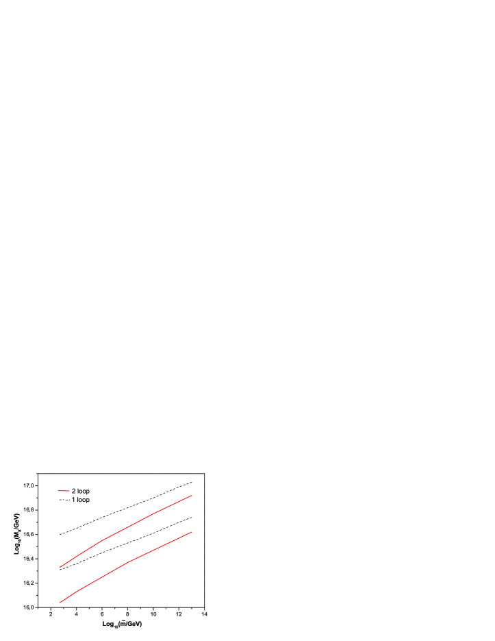
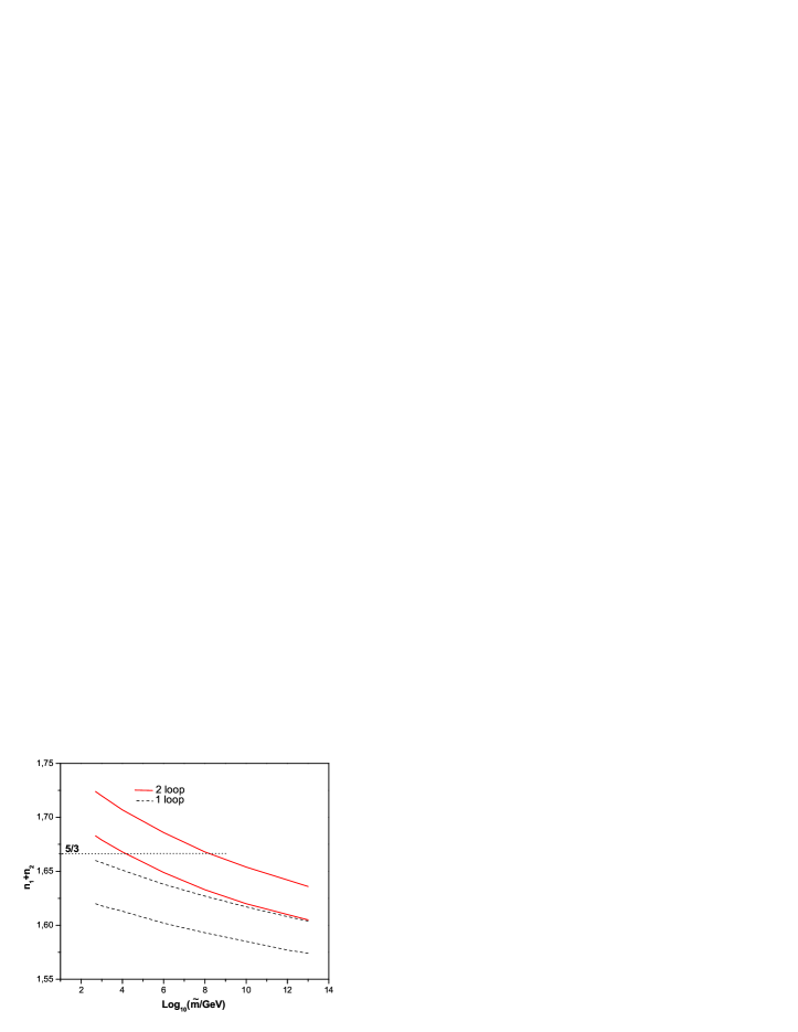
(a)	(b)

Figure 2: The $M_{S}$ scale,(a), and the sum $n_{1}+n_{2}$, (b), as a function of $\log_{10}\tilde{m}$ for the case where $\alpha_{3}=\alpha_{2}$ at $M_{S}$. The bands correspond to the strong coupling experimental error at $M_{Z}$. The solid lines correspond to 2-loop running while the dotted ones to 1-loop.

The $M_{S}$ scale found here is expected to be higher than the corresponding unification scale of the MSSM. This is due to the presence, in the split case and below $\tilde{m}$, of extra degrees of freedom (gauginos and higgsinos) which modify the $\beta$ functions. The width of the band which corresponds to the strong coupling experimental error at $M_{Z}$ corresponds almost to a factor of 2 in the $M_{S}$ scale. This is not at all surprising, since simple calculations in 1-loop approximation show that

$$\ln M_{S}=\ln\tilde{m}+\left(\frac{1}{\alpha_{2}(M_{Z})}-\frac{1}{\alpha_{3}(M_{Z})}\right)\frac{2\pi}{b_{2}^{S}-b_{3}^{S}}-\frac{b_{2}^{SP}-b_{3}^{SP}}{b_{2}^{S}-b_{3}^{S}}\left(\ln\tilde{m}-\ln M_{Z}\right)$$

where the superscript S (SP)to the b-coefficients corresponds to the Susy (Split Susy) case. The difference in $\ln M_{S}$, due to the strong coupling error and for constant m is given by

$$\frac{\Delta^{strong}M_{S}}{M_{S}}=\Delta^{strong}\left(\frac{1}{\alpha_{2}(M_{Z})}-\frac{1}{\alpha_{3}(M_{Z})}\right)\frac{2\pi}{b_{2}^{S}-b_{3}^{S}}=\sim 0.666$$

Figure 3: The $M_{S}$ scale as a function of $n_{1}+n_{2}$. The two curves correspond to the $a_{3}(M_{Z})$ experimental uncertainty. Curves of constant $\tilde{m}$ are shown for the values $10^{2.7}$, $10^{8}$ and $10^{13}$ GeV.

The correlation of the string and Split Susy scales for different values of $k_{Y}$, can be seen in Fig.(3) where, we plot $M_{S}$ as a function of $k_{Y}$. It can be readily seen that the $M_{S}$ value is not very sensitive to the value of $k_{Y}$.

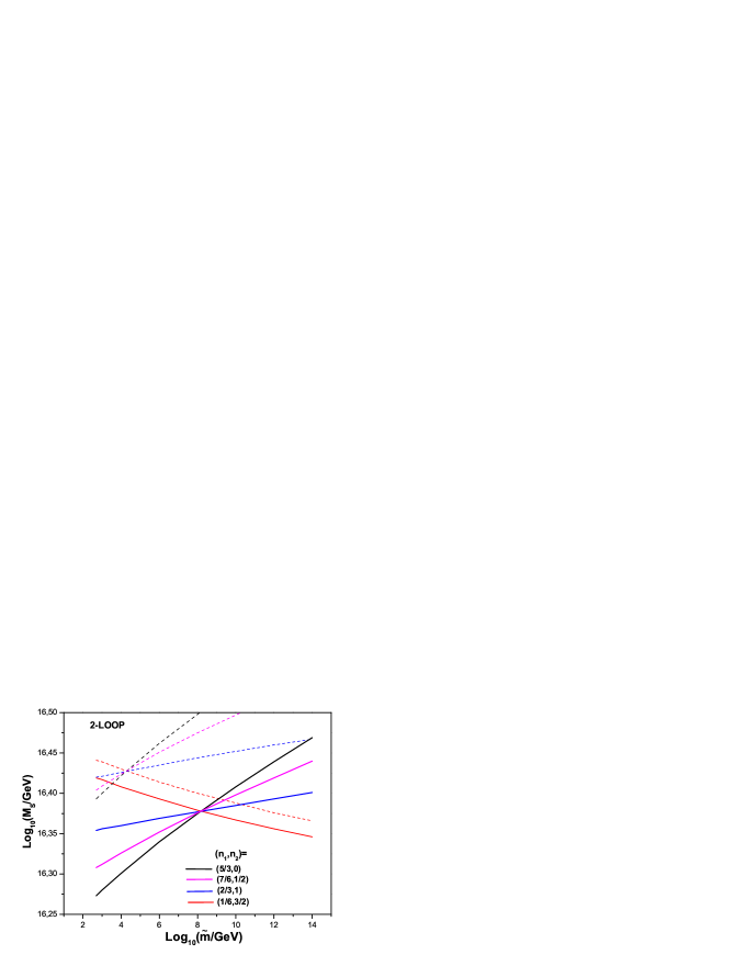
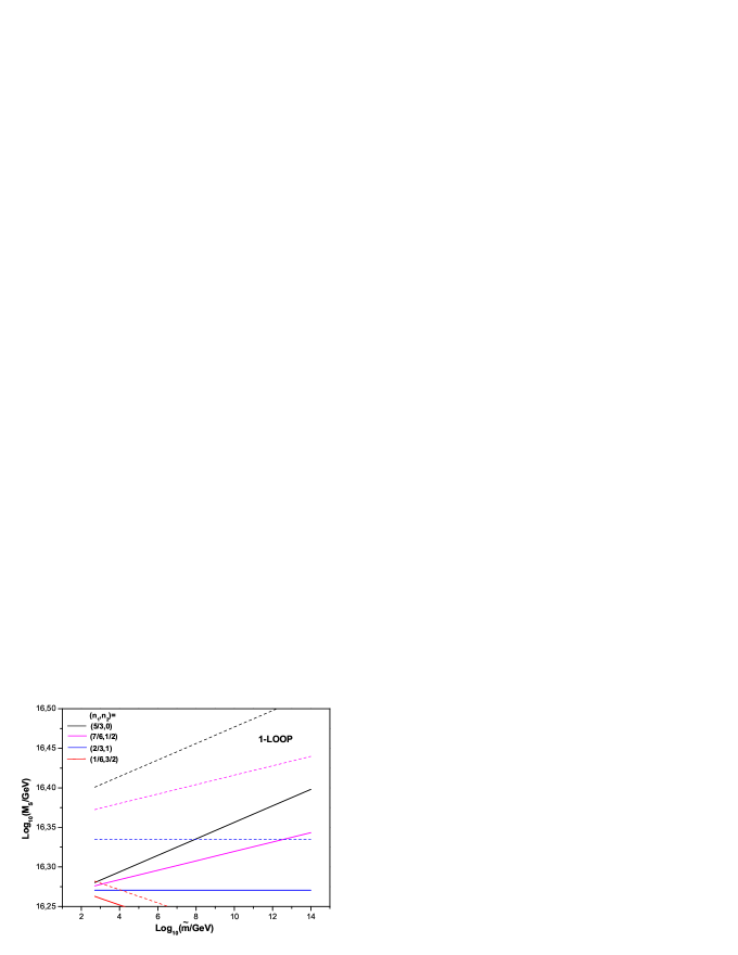
(a)	(b)

Figure 4: The $M_{S}$ scale as a function of $\tilde{m}$, for 2-loop running (a) and 1-loop running (b), for the models having $n_{1}+n_{2}=5/3$. Continuous lines correspond to the lower value of $\alpha_{3}(M_{Z})$ while dotted ones to the higher one.

Next, relaxing the requirement of $SU(3)$ and $SU(2)$ gauge coupling unification, we calculate $M_{S}$ for all models that satisfy the relation $n_{1}+n_{2}=5/3$ as a function of $\tilde{m}$. Since the equality of $\alpha_{2}$ and $\alpha_{3}$ at $M_{S}$ is no longer required, different models evolve differently. The results are depicted in Fig.(4). It is interesting to realize that all the curves have one common point. In other words, there exists a singled out $\tilde{m}$ value that gives the same $M_{string}$ for all models in this class. This is expected as we have seen in our first approach and in Fig.(3): If we choose a specific $\tilde{m}$ scale we can satisfy Eq.(18) at a scale $M_{S}$ with the additional requirement that at this scale $\alpha_{3}=\alpha_{2}$. All models corresponding to a given $n_{1}+n_{2}$ behave similarly. This behavior is independent of 1-loop or 2-loop running, although these special points are different (see Fig.(4(b)). Notice also the big difference (6 orders of magnitude) in the value of $\tilde{m}$ between the corresponding meeting point of 1- and 2-loop running although the difference in $M_{S}$ is much smaller. This point is also made clear in Fig.(2b), where the curves meet the $5/3$ value at very low $\tilde{m}$.

In Fig.(5) we show for the sake of completeness, the corresponding graph for two more models, namely (8/3,1) and (14/3,1). The values for both $M_{S}$ and $\tilde{m}$ are now found to be much smaller than before.

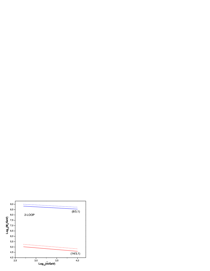
Figure 5: The $M_{S}$ scale as a function of $\tilde{m}$, for 2-loop running for the models with (8/3,1) and (14/3,1). Continuous lines correspond to the lower value of $\alpha_{3}(M_{Z})$ while dotted ones to the higher one.

5 Mirrors

$$\begin{array}[]{|c|c|c|c|c|c|c|c|c|}\hline\cr\textrm{model}&Q&U&D&L&E&N&Y&H\\ \hline\cr 1&0&0&0&0&2&3&2&16\\ \hline\cr 2&0&0&0&0&2&3&6&16\\ \hline\cr 3&0&0&0&2&2&3&6&8\\ \hline\cr 4&0&0&0&2&2&3&6&24\\ \hline\cr 5&0&0&0&6&2&3&2&8\\ \hline\cr 6&0&0&0&6&2&3&2&24\\ \hline\cr 7&2&0&0&0&2&3&2&16\\ \hline\cr 8&2&0&0&0&2&3&6&16\\ \hline\cr 9&4&0&0&2&2&3&2&8\\ \hline\cr 10&4&0&0&2&2&3&2&24\\ \hline\cr 11&4&0&0&6&2&3&6&8\\ \hline\cr 12&4&0&0&6&2&3&6&24\\ \hline\cr\end{array}$$

Table 4: The twelve possible configurations of extra mirror content

As mentioned previously, D-brane constructions include states with the quantum numbers of leptoquarks. Such cases have already been analyzed in the context of CFT-orientifolds models. Here, we will pick up the 32 models presented in [19] which also have the advantage of inducing neutrino Majorana masses through instanton effects. The extra particles of these models consist of mirror states having the same quantum numbers (under the SM gauge group) as the standard ones, with the exception of singlet neutrinos and d-like leptoquarks, i.e. states with the quantum numbers of d-quarks carrying both lepton and baryon number. Four brane-stack configurations are considered in the above construction, two of them carrying the $SU(3)$ and the $SU(2)$, with 2 more providing either a $U(1)$ and an $O(2)$, or two $U(1)$ factors. A similar analysis can also be carried out for the five brane-stack scenario discussed in the present work.

The above 32 models correspond to only 12 distinct spectra with the exotic states shown in Table 4. The doublet and the singlet quarks are denoted by $Q$, $U$ and $D$ respectively, the doublet and the singlet leptons are $L$ and $E$, $N$ are the right-handed neutrinos, $Y$ stands for the leptoquarks and finally, $H$ represents the Higgs. Note that in these models the minimum number of RH neutrinos required is 3 (to avoid the cubic anomaly) however, since these are singlets under the SM gauge group do not contribute to the running of the couplings.

We will now repeat the renormalization group analysis for these models, including also the exotic states. Starting again from the known initial values of the three SM couplings at $M_{Z}$, we determine, for each of the above models, the pair $(\tilde{m},M_{S})$ subject to the “unification” condition (18) at $M_{S}$. Above $\tilde{m}$ we have the complete MSSM spectrum enriched by the extra mirrors appearing in Table 4. Below $\tilde{m}$, we have Split Susy containing extra quarks, leptons, leptoquarks and higgsinos, while we keep one Higgs doublet only as in the original Split scenario. Since our group is the SM one, no extra gauginos appear.

a	b

Figure 6: Plots of $M_{S}$ vs $\tilde{m}$ for the twelve models appearing in Table 4 and the two cases of the pair $(n_{1},n_{2})$. The thicker line corresponds to the case with no mirrors (0 model) while the label corresponds to the model as in Table 4.

In Fig.6 we plot the one-loop results for the 12 models together with the case of no extra mirrors (thick line) and for $(n_{1},n_{2})$ equal to(14/3,1) and (8/3,1) respectively. The allowed region lies above the $\tilde{m}=M_{S}$ line. The emerging picture seems to favor higher $M_{S}$ values as compared to the minimal cases discussed previously. Notice that in models 9 and 10, $\tilde{m}$ is almost fixed ($10^{6.5}$ and $10^{7.5}$) while $M_{string}$ varies along the whole (acceptable) range.

Some comments are here in order. In Fig.6(a), the depicted models can be grouped in three distinctive classes: (i) In the low $M_{S}$ class, the higher $\tilde{m}$ the lower $M_{S}$. (ii) In the class with high $M_{S}$ the tendency is reversed. (iii) The third class has almost constant $\tilde{m}$ while $M_{S}$ varies along the whole (acceptable) range. In Fig.6(b), the majority of the models show that $M_{S}$ is less sensitive against the variation of $\tilde{m}$. This rather peculiar behavior can be easily explained if we recall Eq.(7) written in the form

$$\ln\left[{\frac{{M_{S}}}{{M_{Z}}}}\right]=a\ln\left[{\frac{{\tilde{m}}}{{M_{Z}}}}\right]+b\,\cdot$$

In models of the first class $a<0$. In class (ii) $a>0$ and $M_{S}$ increases with ${\tilde{m}}$. Finally, for models in (iii) $a$ is very large and $M_{S}$ is almost independent of ${\tilde{m}}$.

6 The lepton flavor violating process $\mu\rightarrow e\gamma$

One of the most important flavor violating rare processes present in all models with flavor mixing in the Yukawa sector, is the decay of the muon to an electron-photon pair. In ordinary supersymmetric theories, this exotic process is usually suppressed by powers of the supersymmetry breaking scale which is of the order of 1 TeV at the most [20],[21]. If the scalar partners involved in the process are non-universal, hard violations of the lepton number conservation that exceed the present experimental limits are expected. Even in the case of universal masses at the unification scale, renormalization effects result to mass splitting and important mixing effects at low energies. Although there is a certain degree of ambiguity due to the unknown mixing details in lepton and slepton mass matrices in the calculation of the branching ratios, a significant portion of the universal gaugino mass–universal scalar mass parameter space $(m_{1/2},m_{0})$ is excluded in ordinary supersymmetric models. In the present analysis, we examine the conditions for accessibility of this interesting decay in the context of the D-brane constructions discussed above.

In Split Susy, the scale of the slepton masses is set by the $\tilde{m}$ scale which is considered to be much higher than the TeV ordinary Susy scale. The renormalization group analysis of the generic D-brane constructions has shown however, that in several cases the $\tilde{m}$ can be as low as a few TeV. Graphs for $\mu\rightarrow e\gamma$ are mediated by the above scalars. It is worth exploring whether in some of the above models, these exotic reactions could be observed in future experiments. The branching ratio of the $\mu\rightarrow e\gamma$ process is given by [20, 21]

$$\textrm{BR}(\mu\rightarrow e\gamma)=\frac{48\pi^{3}\alpha}{G_{F}^{2}}\left(|A_{2}^{L}|^{2}+|A_{2}^{R}|^{2}\right)$$

where

$$A_{2}^{L}=A_{2}^{(n)L}+A_{2}^{(c)L}\quad\quad\textrm{and}\quad\quad A_{2}^{R}=A_{2}^{(n)R}+A_{2}^{(c)R}\,\cdot$$

The superscript $n$ ($c$) of the amplitudes $A$ corresponds to the neutralino (chargino) exchange contribution and $L$ ($R$) to the left (right) handed incoming lepton. The amplitudes are given by the relations

$$A_{2}^{(n)L} =\frac{1}{32\pi^{2}}\frac{1}{\tilde{m}^{2}_{\tilde{l}_{X}}}\left[N^{L(l)}_{1AX}N^{L(l)*}_{2AX}\,f_{1}(r)+N^{L(l)}_{1AX}N^{R(l)*}_{2AX}\,\frac{M_{\tilde{\chi}^{0}_{A}}}{m_{\mu}}\,f_{2}(r)\right]$$ (35)

$$A_{2}^{(c)L} =-\frac{1}{32\pi^{2}}\frac{1}{\tilde{m}^{2}_{\tilde{\nu}_{X}}}\left[C^{L(l)}_{1AX}C^{L(l)*}_{2AX}\,f_{3}(r^{\prime})+C^{L(l)}_{1AX}C^{R(l)*}_{2AX}\,\frac{M_{\tilde{\chi}^{-}_{A}}}{m_{\mu}}\,f_{4}(r^{\prime})\right]$$ (36)

$$A_{2}^{(n)R} =A_{2}^{(n)L}|_{L\leftrightarrow R}\quad\quad\textrm{and}\quad\quad A_{2}^{(c)R}=A_{2}^{(c)L}|_{L\leftrightarrow R}\,\cdot$$ (37)

We are working with the mass eigenstates so, all matrices rotating from the weak to the mass eigenstates are moved to the vertices. The neutral amplitude involves the neutralinos and the charged sleptons with corresponding masses $M_{\tilde{\chi}^{0}_{A}}$ ($A=1,...,4$) and $\tilde{m}_{\tilde{l}_{X}}$ ($X=1,...,6$) while $m_{\mu}$ is the mass of the decaying muon. The charged amplitude involves the charginos and sneutrinos with corresponding masses $M_{\tilde{\chi}^{-}_{A}}$ ($A=1,2$) and $\tilde{m}_{\tilde{\nu}_{X}}$ ($X=1,2,3$). The matrices $N^{L(l)}_{iAX}$ and $N^{R(l)}_{iAX}$ involve both the neutralino and the slepton rotating matrices ($i=1$ for the electron and $i=2$ for the muon) and are given by

$$\begin{split}N^{R(l)}_{iAX}&=-\frac{g_{2}}{\sqrt{2}}\left\{\left[-(O_{N})_{A2}-(O_{N})_{A1}\tan\theta_{W}\right]U^{l}_{Xi}+\frac{m_{i}}{m_{W}\cos\beta}\,(O_{N})_{A3}U^{l}_{X(i+3)}\right\}\\ N^{L(l)}_{iAX}&=-\frac{g_{2}}{\sqrt{2}}\left\{\frac{m_{i}}{m_{W}\cos\beta}\,(O_{N})_{A3}U^{l}_{Xi}+2(O_{N})_{A1}\tan\theta_{W}U^{l}_{X(i+3)}\right\}\,\cdot\end{split}$$

The matrices $O_{N}$ rotate the neutralinos while $U^{l}$ rotate the charged sleptons. Finally, $m_{i}$ is the lepton mass ($m_{1}=m_{e}$, $m_{2}=m_{\mu}$).

The matrices $C^{L(l)}_{iAX}$ and $C^{L(l)}_{iAX}$ (again $i=1$ for the electron and $i=2$ for the muon) involve both the chargino ($O_{L}$ and $O_{R}$) and the sneutrino ($U^{\nu}$) rotating matrices and they are given by

$$\begin{split}C^{R(l)}_{iAX}&=-g_{2}(O_{R})_{A1}U^{\nu}_{Xi}\\ \\ C^{L(l)}_{iAX}&=g_{2}\,\frac{m_{i}}{\sqrt{2}m_{W}\cos\beta}(O_{L})_{A2}U^{\nu}_{Xi}\,\cdot\end{split}$$

Finally, the $f$ functions appearing in Eqs.(35) and (36) are

$$\begin{split}f_{1}(r)&=\frac{1}{6(1-r)^{4}}(1-6r+3r^{2}+2r^{3}-6r^{2}\ln(r))\\ f_{2}(r)&=\frac{1}{(1-r)^{3}}(1-r^{2}+2r\ln(r))\\ f_{3}(r^{\prime})&=\frac{1}{6(1-r^{\prime})^{4}}(2+3r^{\prime}-6r^{\prime 2}+r^{\prime 3}+6r^{\prime}\ln(r^{\prime}))\\ f_{4}(r^{\prime})&=\frac{1}{(1-r)^{3}}(-3+4r^{\prime}-r^{\prime 2}-2\ln(r^{\prime}))\\ \textrm{where,}\quad r&=\frac{M^{2}_{\tilde{\chi}^{0}_{A}}}{\tilde{m}^{2}_{\tilde{l}_{X}}}\quad\quad\textrm{and}\quad\quad r^{\prime}=\frac{M^{2}_{\tilde{\chi}^{-}_{A}}}{\tilde{m}^{2}_{\tilde{\nu}_{X}}}\,\cdot\end{split}$$

In estimating the $\mu\rightarrow e\gamma$ branching ratio and in order not to complicate our analysis we have ignored the neutralino and the chargino mixing (i.e. the $O_{L}$, $O_{R}$ and $O_{N}$ matrices are the identity matrix) and have dropped terms proportional to the mass of the leptons. Therefore, we are left with the $U^{l}$ and $U^{\nu}$ matrices.

The $6\times 6$ charged slepton matrix is given by

$$\left(\begin{array}[]{cc}m^{2}_{LL}&m^{2}_{LR}\\ m^{2}_{RL}&m^{2}_{RR}\\ \end{array}\right)$$ (38)

where each entry is a $3\times 3$ matrix with an obvious notation and [22]

$$m^{2}_{LL} =(\tilde{m}^{\delta}_{\tilde{l}})^{2}+\delta m^{2}_{N}+m^{2}_{l}+M^{2}_{Z}\left(\frac{1}{2}-\sin^{2}\theta_{W}\right)\cos 2\beta$$ (39)

$$m^{2}_{RR} =(\tilde{m}^{\delta}_{\tilde{e}_{R}})^{2}+m^{2}_{l}-M^{2}_{Z}\sin^{2}\theta_{W}\cos 2\beta$$ (40)

$$m^{2}_{RL} =(A_{e}^{\delta}+\delta A_{e}+\mu\tan\beta)m_{l}$$ (41)

$$m^{2}_{LR} =m^{2{\dagger}}_{RL}\,\cdot$$ (42)

The superscript $\delta$ denotes the diagonal part of the corresponding $3\times 3$ matrix and we have assumed universal soft masses, so that $(\tilde{m}^{\delta}_{\tilde{l}})^{2}=(\tilde{m}^{\delta}_{\tilde{e}_{R}})^{2}=\textrm{Diagonal}(m_{0},m_{0},m_{0})$ where in our case, $m_{0}=\tilde{m}$. Also, $A_{e}^{\delta}=\textrm{Diagonal}(A_{0},A_{0},A_{0}))$ with $A_{0}=-1.5m_{0}$. The terms $\delta m^{2}_{N}$ and $\delta A_{e}$ stand for the off-diagonal matrices which arise because of the non-diagonal Yukawa coupling $\lambda_{D}$ (in the basis where the lepton matrix is diagonal) appearing in the term which gives mass to the neutrino through the superpotential term $N^{c}\lambda_{D}lH_{2}$ and in the trilinear coupling of the potential correspondingly. The sneutrino reduced $3\times 3$ matrix ([22]) is given by

$$\tilde{m}^{2}_{\tilde{\nu}}=(\tilde{m}^{\delta}_{\tilde{l}})^{2}+\delta m^{2}_{N}+\frac{1}{2}M^{2}_{Z}\cos 2\beta\,\cdot$$ (43)

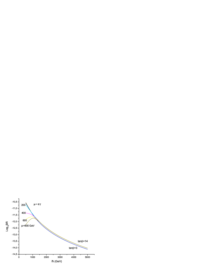
Figure 7: The (logarithm of the) branching ratio of $\mu\rightarrow e\gamma$ as a function of $\tilde{m}$ for $\tan\beta=3$ and 14 and for $\mu=200,400,600,800$ GeV.

The off diagonal matrices $\delta m^{2}_{N}$ and $\delta A_{e}$ are evaluated in [22] for the region of $\tan\beta=3-14$. Having determined the mass matrices for the charged sleptons and the sneutrino, we can find the matrices $U^{l}$ and $U^{\nu}$ which rotate to the corresponding mass eigenstates and therefore, proceed to the evaluation of the desired branching ratio. In Fig.(7) we show the BR as a function of $\tilde{m}$ for the above region of $\tan\beta$ and for $\mu=200-800$ GeV. We clearly see that for the present experimental BR bound ($10^{-12}$), $\mu\rightarrow e\gamma$ could be observed in models allowing $\tilde{m}$ around 1.5 TeV (for the evaluation of the BR we have assumed a universal gaugino mass of 200 GeV, since we run our RGE’s with the Split Susy regime active down to the weak scale).

From the renormalization group analysis of the previous section, we can check that for a wide class of D-brane constructions, the Split-supersymmetric scale ranges from 1 TeV up to values as high as $10^{13}$ GeV. The above reaction could in principle be observed in the present day experiments for the lower marginal values of the Split Susy scale as it can also be seen from Fig. 2 and 3. However, if we stick to cases where we have $a_{3}=a_{2}$ unification at $M_{S}$, the $U(1)_{Y}$ normalization constant $k_{Y}$ is found to be around the standard value $\frac{5}{3}$. Then, from Fig. 3 we observe that $\tilde{m}\sim 10^{8}$ GeV therefore, the branching ratio is significantly suppressed and lies far beyond the capabilities of even future experiments.

On the other hand, the observability prospects of this reaction are different in models implying low string scale, since the Split scale $\tilde{m}$ cannot be higher that $\tilde{m}\leq M_{S}\sim 5$ TeV. For $\tilde{m}\sim 5$ TeV, the ${\mu\rightarrow e\gamma}$ branching ratio is $BR_{\mu\rightarrow e\gamma}\sim 10^{-14}$, a number that could in principle be checked in future experiments. Thus, for this particular class of D-brane constructions, muon number violating reactions can probe the whole $\tilde{m}$-region.

7 Conclusions

D-branes brought profound changes in our approach to model building. In the present work, we presented the simplest D-brane extensions of the Standard Model based on configurations with gauge symmetry of the form $U(3)\times U(2)\times U(1)^{P}$ with $P\leq 3$. Exploring the different brane-stack orientations in the higher dimensional space as well as the various hypercharge embeddings consistent with the SM particle spectrum, we managed to obtain a complete classification of the SM variants that arise in this context. We addressed several phenomenological issues affecting the viability of these constructions. These issues were examined in the context of split supersymmetric spectrum which has been shown to be a natural possibility in a wide class of D-brane constructions. This way, we extended previous investigations on the correlation between the string scale and the split supersymmetry breaking scale, incorporating two-loop effects. The calculations show a significant change on the split supersymmetry breaking scale as compared to the one-loop results, while, the string scale for several interesting cases is only moderately affected. The analysis was further extended to non-minimal cases that include leptoquark and mirror states. Yukawa terms providing masses to the SM fields were calculated, while the problem of incorporating the right handed neutrino mass through instanton effects was also mentioned. Finally, we presented a detailed discussion on the possible observability of the $\mu\rightarrow e\gamma$ flavor violating decay in the present and future experiments.

The work is partially supported by the EU Grant MRTN-CT-2004-503369.

References

- [1] J. Polchinski, “Dirichlet-Branes and Ramond-Ramond Charges”, Phys. Rev. Lett. 75 (1995) 4724 [arXiv:hep-th/9510017].
- [2] R. Blumenhagen, M. Cvetic, P. Langacker and G. Shiu, “Toward realistic intersecting D-brane models”, Ann. Rev. Nucl. Part. Sci. 55 (2005) 71 [arXiv:hep-th/0502005].
- [3] R. Blumenhagen, B. Kors, D. Lust and S. Stieberger, “Four-dimensional String Compactifications with D-Branes, Orientifolds and Fluxes”, arXiv:hep-th/0610327.
- [4] I. Antoniadis, E. Kiritsis and T. Tomaras, “D-brane Standard Model”, Fortsch. Phys. 49 (2001) 573 [arXiv:hep-th/0111269].
- [5] I. Antoniadis, E. Kiritsis, J. Rizos and T. N. Tomaras, “D-branes and the standard model”, Nucl. Phys. B 660 (2003) 81 [arXiv:hep-th/0210263].
- [6] D. V. Gioutsos, G. K. Leontaris and J. Rizos, “Gauge coupling and fermion mass relations in low string scale brane models”, Eur. Phys. J. C 45 (2006) 241 [arXiv:hep-ph/0508120].
- [7] P. Anastasopoulos, T. P. T. Dijkstra, E. Kiritsis and A. N. Schellekens, “Orientifolds, hypercharge embeddings and the standard model”, Nucl. Phys. B 759 (2006) 83 [arXiv:hep-th/0605226].
- [8] D. V. Gioutsos, G. K. Leontaris and A. Psallidas, “D-brane standard model variants and split supersymmetry: Unification and fermion mass predictions”, Phys. Rev. D 74 (2006) 075007 [arXiv:hep-ph/0605187].
- [9] R. Blumenhagen, L. Goerlich, B. Kors and D. Lust, “Noncommutative compactifications of type I strings on tori with magnetic background flux”, JHEP 0010 (2000) 006 [arXiv:hep-th/0007024].
- [10] G. Aldazabal, S. Franco, L. E. Ibanez, R. Rabadan and A. M. Uranga, “Intersecting brane worlds”, JHEP 0102 (2001) 047 [arXiv:hep-ph/0011132].
- [11] E. Kiritsis, “D-branes in standard model building, gravity and cosmology”, Fortsch. Phys. 52 (2004) 200 [Phys. Rept. 421 (2005 ERRAT,429,121-122.2006) 105] [arXiv:hep-th/0310001].
- [12] N. Arkani-Hamed and S. Dimopoulos, “Supersymmetric unification without low energy supersymmetry and signatures for fine-tuning at the LHC”, JHEP 0506 (2005) 073 [arXiv:hep-th/0405159].
- [13] T. Gherghetta and A. Pomarol, “The standard model partly supersymmetric”, Phys. Rev. D 67 (2003) 085018 [arXiv:hep-ph/0302001].
- [14] I. Antoniadis and S. Dimopoulos, “Splitting supersymmetry in string theory”, Nucl. Phys. B 715 (2005) 120 [arXiv:hep-th/0411032].
- [15] G. F. Giudice and A. Romanino, “Split supersymmetry”, Nucl. Phys. B 699 (2004) 65 [Erratum-ibid. B 706 (2005) 65] [arXiv:hep-ph/0406088].
- [16] V. Barger, P. Langacker and G. Shaughnessy, “TeV physics and the Planck scale”, arXiv:hep-ph/0702001.
- [17] D. Cremades, L. E. Ibanez and F. Marchesano, “Yukawa couplings in intersecting D-brane models,” JHEP 0307 (2003) 038 [arXiv:hep-th/0302105].
-
[18]
R. Blumenhagen, M. Cvetic and T. Weigand,
“Spacetime instanton corrections in 4D string vacua: The Seesaw
mechanism for D-Brane models”,
arXiv:hep-th/0609191.
L. E. Ibanez and A. M. Uranga, “Neutrino Majorana masses from string theory instanton effects”, JHEP 0703 (2007) 052 [arXiv:hep-th/0609213].
M. Cvetic, R. Richter and T. Weigand, “Computation of D-brane instanton induced superpotential couplings: Majorana masses from string theory”, arXiv:hep-th/0703028. - [19] L. E. Ibanez, A. N. Schellekens and A. M. Uranga, “Instanton Induced Neutrino Majorana Masses in CFT Orientifolds with MSSM-like spectra”, arXiv:0704.1079 [hep-th].
-
[20]
J. Hisano, T. Moroi, K. Tobe and M. Yamaguchi,
“Lepton-Flavor Violation via Right-Handed Neutrino Yukawa Couplings in
Supersymmetric Standard Model,”
Phys. Rev. D 53 (1996) 2442
[arXiv:hep-ph/9510309].
J. Hisano and D. Nomura, “Solar and atmospheric neutrino oscillations and lepton flavor violation in supersymmetric models with the right-handed neutrinos”, Phys. Rev. D 59 (1999) 116005 [arXiv:hep-ph/9810479].
J. A. Casas and A. Ibarra, “Oscillating neutrinos and ”, Nucl. Phys. B 618 (2001) 171 [arXiv:hep-ph/0103065]. -
[21]
J. R. Ellis, M. E. Gomez, G. K. Leontaris, S. Lola and D. V. Nanopoulos,
“Charged lepton flavour violation in the light of the Super-Kamiokande
data”,
Eur. Phys. J. C 14 (2000) 319
[arXiv:hep-ph/9911459].
G. K. Leontaris and N. D. Tracas, “Lepton flavour violation in unified models with U(1)-family symmetries”, Phys. Lett. B 431 (1998) 90 [arXiv:hep-ph/9803320].
T. Kosmas, G. K. Leontaris and J. D. Vergados, “Lepton flavor violation in Supergravity theories”, Phys. Lett. B 219 (1989) 457. - [22] M. E. Gomez, G. K. Leontaris, S. Lola and J. D. Vergados, “U(1)-textures and lepton flavor violation”, Phys. Rev. D 59 (1999) 116009 [arXiv:hep-ph/9810291].