Weak values of electron spin in a double quantum dot

Abstract

We propose a protocol for a controlled experiment to measure a weak value of the electron’s spin in a solid state device. The weak value is obtained by a two step procedure – weak measurement followed by a strong one (post-selection), where the outcome of the first measurement is kept provided a second post-selected outcome occurs. The set-up consists of a double quantum dot and a weakly coupled quantum point contact to be used as a detector. Anomalously large values of the spin of a two electron system are predicted, as well as negative values of the total spin. We also show how to incorporate the adverse effect of decoherence into this procedure.

Introduction.— The measurement of any observable in quantum mechanics is a probabilistic process described by the projection postulate von Neuman (1932). Each eigenvalue of the observable happens to be an outcome of the measurement process with a given probability, and the original state of the system collapses into the corresponding eigenstate. An intriguing viewpoint of quantum mechanics, based on a two-vector formulation Aharonov et al. (1964), stipulates that the measured value of an observable depends on both a “past vector”, $\left|\chi_{0}\right\rangle$, at which the system is prepared (pre-selection), and a “future vector”, $\left|\chi_{f}\right\rangle$, where a given state is selected following the measurement (post-selection). Within this framework a procedure that leads to a weak value (WV) Aharonov et al. (1988) involves a weak measurement (i.e. a measurement that disturbs the system weakly) whose outcome is kept provided a second postselected outcome occurs. The protocol for the WV of $\hat{A}$, ${}_{f}\langle\hat{A}\rangle_{0}^{(W)}=\langle\chi_{f}|\hat{A}|\chi_{0}\rangle/\langle\chi_{f}|\chi_{0}\rangle$ Aharonov et al. (1988); Aharonov and Vaidman (1990), involves three steps: (i) preselection, (ii) weak measurement of $\hat{A}$, and then (iii) projective post-selection of an eigenstate of observable $\hat{B}$. WVs can be orders of magnitude larger than strong values Aharonov et al. (1988), negative (where conventional strong values would be positive definite) 200 (2002), or even complex. Such non-standard values open an intriguing window to some fundamental aspects of quantum measurement, including access to simultaneous measurement of non-commuting variables non_commuting ; dephasing and phase recovery Neder et al. (2007); correlation between measurements correlations ; and even new horizons in metrology Aharonov et al. (1988).

While some aspects of WVs have been demonstrated in optics based setups optics , the arena of quantum solid state offers very rich physics to be studied through a WV measurement, and the possibility to fine tune and control the system’s parameters through electrostatic gates and an applied magnetic field. The three main challenges in such an undertaking are: (1) overcoming the adverse effects of dephasing during the application of the protocol, (2) designing a tunable detector that will operate in both the strong and weak measurement regimes, (3) design a protocol such that step (ii) and (iii) do not commute,

$$[\hat{A},\hat{B}]\neq 0\,,$$ (1)

notwithstanding the fact that both $\hat{A}$ and $\hat{B}$ address the charge degree of freedom.

Here we propose a protocol for a controlled experiment to measure the weak value of the electron’s spin. Our protocol overcomes the above mentioned difficulties. We also show how to incorporate the adverse effect of decoherence into this procedure. The set-up consists of a double quantum dot, recently studied as a candidate for a quantum computer qubit Petta et al. (2005), and a weakly coupled quantum point contact to be used as a detector.

Within the protocol alluded to above, the interaction between the detector (D) and the system (S) is weak in the coupling parameter $\lambda\ll 1$. As a result of the weak measurement, the shift in the detector’s coordinate, $q$, is $\propto\lambda$, while the modification of the state of the system is $\propto\lambda^{2}$, hence $\left|\chi_{0}\right\rangle$ is unchanged to order $\lambda$. In an ideal strong measurement there is a one-to-one correspondence between the observed value of the detector’s coordinate, $q_{\alpha}$, and the state of S, $\left|\alpha\right\rangle$. Within a weak measurement procedure the ranges of values of $q$ that correspond to two distinct states of S, $\left|\alpha\right\rangle$ and $\left|\alpha^{\prime}\right\rangle$, are described by two probability distribution functions, $P_{\alpha}(q)$ and $P_{\alpha^{\prime}}(q)$ respectively. These distributions strongly overlap. Hence the measurement of $q$ provides only partial information on the state of S.

The model.— Petta et al. Petta et al. (2005) studied experimentally a device that can operate and be controlled over time scales up to tens of nanoseconds or more, preserving quantum coherence. This system (cf. Fig. 1(a)) consists of a gate confined semiconducting double quantum dot hosting two electrons.

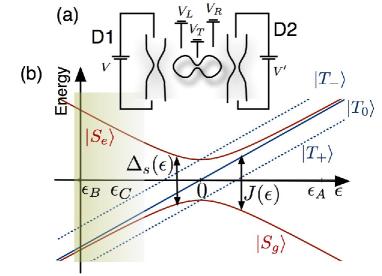
Figure 1: (Color online) Schematics of the system and energy levels. (a) Scheme of a double dot with nearby quantum point contacts (QPCs) as charge sensors. (b) Energy levels of lowest singlet (red) and triplet (blue) states vs. the detuning parameter $\epsilon$. In the $(0,2)$ charge configuration the antisymmetric nature of the electrons wave function implies a singlet ground state. The states $\left|T_{\pm}\right\rangle$ (blue dashed lines), with angular momenta $\pm\hbar$ in the direction of the applied magnetic field, are split by the Zeeman energy ($\Delta=g\mu_{B}B\approx 2.5\mu eV$ in Ref. 4). The range of $\epsilon$ in which the effect of nuclear interaction is relevant is highlighted by the shadowed part. Spin-to-charge conversion. If the variation $\epsilon_{B}\rightarrow\epsilon_{A}$ is fast on the time scale of the nuclear field coupling, $\langle T_{0}(1,1)|H_{N}|S(1,1)\rangle$, (”fast adiabatic”), $\left|S(1,1)\right\rangle$ is mapped into the ground state, $\left|S(0,2)\right\rangle$. For the ”slow adiabatic” limit the ground state of the total Hamiltonian, $\left|\uparrow\downarrow\right\rangle$, will be mapped into $\left|S(0,2)\right\rangle$. By measuring the charge of the final state one is effectively measuring either the singlet, triplet or the $\left|\uparrow\downarrow\right\rangle$, $\left|\downarrow\uparrow\right\rangle$ component of the initial state at $\epsilon=\epsilon_{B}$, depending on the specific time sequence of $\epsilon$.

The charge configuration in the two dots, $(n_{L},n_{R})$, is controlled by the gate voltages $V_{L}$ and $V_{R}$. In particular, by controlling the dimensionless parameter $\epsilon\propto V_{R}-V_{L}$, the charge configuration is continuously tuned between $(0,2)$ and $(1,1)$. When the two electrons are in the same dot $(0,2)$, the ground state is a spin singlet, $\left|S(0,2)\right\rangle$; the highly energetic excited triplet states are decoupled. For $(1,1)$ the degeneracy of the triplet states is removed by a magnetic field, $\textbf{B}=B\hat{\textbf{z}}$, applied perpendicularly to the sample’s plane; $\left|S(1,1)\right\rangle$ and $\left|T_{0}(1,1)\right\rangle$ are degenerate. The charging energy and the spin preserving inter-dot tunneling (controlled by the gate voltage $V_{T}$) are described by $H_{0}=\Delta_{s}(0)[\epsilon(\left|T_{0}(1,1)\right\rangle\left\langle T_{0}(1,1)\right|+\left|S(1,1)\right\rangle\left\langle S(1,1)\right|-\left|S(0,2)\right\rangle\left\langle S(0,2)\right|)+1/2(\left|S(0,2)\right\rangle\left\langle S(1,1)\right|+\textrm{H.c.})]$, where $\Delta_{s}(0)/2$ is the tunneling amplitude. The singlet ground state, $\left|S_{g}(\epsilon)\right\rangle$, and the excited state, $\left|S_{e}(\epsilon)\right\rangle$, together with $\left|T_{0}(1,1)\right\rangle$, diagonalize the Hamiltonian (cf. Fig. 1(b))

$$H_{0}= \Delta_{s}(\epsilon)/2\left(\left|S_{e}(\epsilon)\right\rangle\left\langle S_{e}(\epsilon)\right|-\left|S_{g}(\epsilon)\right\rangle\left\langle S_{g}(\epsilon)\right|\right)$$ (2)

$$+\Delta_{s}(0)\epsilon\left|T_{0}(1,1)\right\rangle\left\langle T_{0}(1,1)\right|\,.$$

The energy gap, $J(\epsilon)=\Delta_{s}(\epsilon)/2+\epsilon\Delta_{s}(0)$, between $\left|S_{g}(\epsilon)\right\rangle$ and $\left|T_{0}(1,1)\right\rangle$ is vanishingly small at $\epsilon\lesssim\epsilon_{B}$ (cf. Fig. 1(b)). The hyperfine interaction between electrons and the nuclear spin nuclei , facilitates transitions between these states. For our purpose, the effect of the nuclear spins on the electrons is described by classical magnetic fields, ${{\bf B}_{N}}_{L}$, ${{\bf B}_{N}}_{R}$, resulting in the Hamiltonian $H_{N}=g\mu_{B}({{\bf B}_{N}}_{R}-{{\bf B}_{N}}_{L})\cdot\hat{{\bf z}}\left|T_{0}(1,1)\right\rangle\left\langle S(1,1)\right|+\textrm{H.c.}$.

Dealing with the spin degree of freedom enables us to achieve long dephasing times, which allows for weak (continuous) measurements Jordan et al. (2007). By contrast, the detectors (D1 and D2), which are two quantum point contacts (QPCs) located near the dots, are charge sensors  sensing suitable for continuous measurements Korotkov:2001aa . D2 is effectively used to perform a strong measurement of the spin, following a spin-to-charge conversion, i.e. a mapping of different spin states at $\epsilon=\epsilon_{B}$ into different charge states at $\epsilon=\epsilon_{A}$, employing an adiabatic (as compared to the tunneling Hamiltonian) variation of $\epsilon$ (cf. Fig. 1). D1 is used as a weak detector. It is sensitive to the difference between two spin states; the latter correspond to two different charge configurations. This is indeed the case for $\epsilon\neq\epsilon_{B}$. The interaction between the double QD and the QPC is modeled as $H_{\textrm{int}}=(H_{(0,2)}-H_{(0,1)})\otimes\left|S(0,2)\right\rangle\left\langle S(0,2)\right|+H_{(1,1)}\otimes{\rm 1}{\rm I}\hskip 1.42262pt$. For the $(1,1)$ (or $(0,2)$) charge configuration, the electrons in the QPC are described by the Hamiltonian $H_{(1,1)}$ (or $H_{(0,2)}$). Assuming the excited singlet state is not populated (which is the case for $k_{B}T$, $eV$, $\hbar/\tau\ll\Delta_{s}(\epsilon)$, cf. Fig. 1(b)), the interaction Hamiltonian can be written as $H_{\textrm{int}}\approx H_{(1,1)}+J(\epsilon)/\Delta_{s}(\epsilon)(H_{(0,2)}-H_{(1,1)})\otimes({\rm 1}{\rm I}\hskip 1.42262pt-\hat{S}^{2}/2)$, where the measured observable, $\hat{A}\equiv{\rm 1}{\rm I}\hskip 1.42262pt-\hat{S}^{2}/2=\left|S_{g}(\epsilon)\right\rangle\left\langle S_{g}(\epsilon)\right|$, is the singlet component of the spin state. $H_{(1,1)}$ describes scattering of the electrons in the QPC with transmission (reflection) coefficient $t_{0}$ ($r_{0}$): any incoming electron in the QPC, $\left|\textrm{in}\right\rangle$, evolves to $\left|\phi\right\rangle=t_{0}\left|t\right\rangle+r_{0}\left|r\right\rangle$, where $\left|t\right\rangle$ and $\left|r\right\rangle$ are the reflected and transmitted states for the electron. If the system is in the $\left|S_{g}(\epsilon)\right\rangle$ state, the electron in the QPC evolves according to $\left|\textrm{in}\right\rangle\rightarrow\left|\phi^{\prime}\right\rangle=(t_{0}+\delta t(\epsilon))\left|t\right\rangle+(r_{0}+\delta r(\epsilon))\left|r\right\rangle=\left|\phi\right\rangle+\left|\Delta\phi\right\rangle$. $\delta t$, $\delta r$ can be tuned to be arbitrarily small in $J(\epsilon)/\Delta_{s}(\epsilon)$.

The protocol.— The protocol consists of a weak measurement with post-selection realized by a sequence of voltage pulses as described in Fig. 2(a).

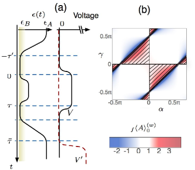
Figure 2: (Color online) (a) A protocol to measure weak values of two electron spin: shown are $V$, $V^{\prime}$, (voltage bias across D1 and D2 respectively) and $\epsilon$. (b) The weak value, ${}_{f}\langle\hat{A}\rangle_{0}^{(W)}=[1-{}_{f}\langle\hat{S}^{2}\rangle_{0}^{(W)}]/2$, as a function of the parameters $\alpha$ and $\gamma$ for $\beta=\pi$. The dark region defines the range of parameters for which a positive post-selection is obtained with probability $P_{(0,2)}<0.5\%$. The shadowed region (parallel lines) corresponds to the values of the parameters for which ${}_{f}\langle\hat{S}^{2}\rangle_{0}^{(W)}<0$.

The evolution of the system in the absence of the detector has already been realized in experiment Petta et al. (2005). Initially, at $\epsilon=\epsilon_{A}$, the system is in the ground state, $\left|S(0,2)\right\rangle$. By a fast adiabatic variation (cf. Fig. 1) it is evolved into $\left|S(1,1)\right\rangle$ ($\epsilon=\epsilon_{B}$ at time $t=-\tau^{\prime}$). This state evolves under the influence of the nuclear interaction until time $t=0$, thus preselecting $\left|\chi_{0}\right\rangle=\cos\alpha\left|S_{g}\right\rangle-i\sin\alpha\left|T_{0}\right\rangle$ with $\alpha=g\mu_{B}({{\bf B}_{N}}_{R}-{{\bf B}_{N}}_{L})\cdot\hat{{\bf z}}\tau^{\prime}$. During the measurement pulse the free evolution of the system is $\mathcal{U}(\tau,0)=\left|S_{g}\right\rangle\left\langle S_{g}\right|+\exp(-i\beta)\left|T_{0}\right\rangle\left\langle T_{0}\right|$, with $\beta=J(\epsilon)\tau$. The evolution during the time interval $(\tau,\tau+\tau^{\prime\prime})$ is governed by the nuclear interaction and that from $\tau+\tau^{\prime\prime}$ to $\bar{\tau}$ is a fast adiabatic variation. The evolution $\mathcal{U}(\bar{\tau},\tau)$ defines the effective post-selected state $|\chi_{f}^{\prime}\left.\right\rangle=\mathcal{U}^{-1}(\bar{\tau},\tau)\left|S(0,2)\right\rangle=\cos\gamma\left|S_{g}\right\rangle+i\sin\gamma\left|T_{0}\right\rangle$, where $\gamma=g\mu_{B}({\bf B}_{NR}-{\bf B}_{NL})\cdot\hat{{\bf z}}\tau^{\prime\prime}$ (cf. Fig. 2(b)). The weak value of $\mathcal{U}(\tau,0)\hat{A}$ is then ${}_{f}\langle\hat{A}\rangle_{0}^{(W)}=\cos\gamma\cos\alpha/(\cos\gamma\cos\alpha-e^{-i\beta}\sin\gamma\sin\alpha)$. By tuning the duration of the pulses, one can obtain a real WV (e.g. for $\beta=\pi$), which is arbitrarily large (e.g. for $\gamma-\alpha\rightarrow\pi/2$) –cf. Fig. 2(b).

The interaction with the detector in this protocol is depicted by a simple model, in which the electrons in the double dot interact with a single electron in the QPC. Once the state $\left|\chi_{0}\right\rangle$ is prepared at time $t=0$, the system interacts with the QPC, $t\in[0,\tau]$, creating an entangled state at time $t=\tau$, $\left|\psi\right\rangle=\mathcal{U}(\tau,0)\left|\chi_{0}\right\rangle\left|\phi\right\rangle+\hat{A}\mathcal{U}(\tau,0)\left|\chi_{0}\right\rangle\left|\Delta\phi\right\rangle$, where $\mathcal{U}(\tau,0)$ defines the time evolution of the system from $t=0$ to $t=\tau$. Applying the operator $\Pi_{t}\equiv\left|t\right\rangle\left\langle t\right|$ one can now detect whether the electron in the QPC has ($n=1$) or has not ($n=0$) been transmitted. The respective probabilities are $P(n=1)=\langle\psi|\Pi_{t}|\psi\rangle$, $P(n=0)=1-P(n=1)$. In either case, the corresponding spin state of the system is given by $\left|\bar{\chi}_{n}\right\rangle=[\Pi_{t}^{n}+(1-\Pi_{t})^{(1-n)}]\left|\psi\right\rangle/\sqrt{\langle\psi|\Pi_{t}|\psi\rangle}$. We employ QPC D2 to detect the charge configuration in the double dot (post selection) at a later time $\bar{\tau}$ (cf. Fig. 2(a)), but use time $t=\tau$ to express the post-selected state, $|\chi_{f}^{\prime}\rangle=\mathcal{U}^{-1}(\bar{\tau},\tau)\left|\chi_{f}\right\rangle$, in terms of the time evolved state, $\left|\chi_{f}\right\rangle$ at time $t=\bar{\tau}$. The signal of QPC D1 is kept, provided D2 measures the $(0,2)$ charge configuration (with probability $P((0,2)|n)=|\langle\bar{\chi}_{n}|\chi_{f}\rangle|^{2}$). This corresponds to averaging the reading of the first QPC conditional to the positive outcome ($(0,2)$ charge configuration) of the second measurement, ${}_{f}\langle n\rangle_{0}=\sum_{n=0,1}nP(n)P((0,2)|n)/(\sum_{n}P(n)P((0,2)|n))$. If $\mbox{\rm Re}\{{}_{f}\langle\hat{A}\rangle_{0}^{(W)}t_{0}^{*}\delta t\}\ll 1$, the average number of transmitted electrons is

$${}_{f}\langle n\rangle_{0}=\left|t_{0}\right|^{2}+2\mbox{\rm Re}\left\{{}_{f}\langle\hat{A}\rangle_{0}^{(W)}t_{0}^{*}\delta t\right\}\,,$$

$${}_{f}\langle\hat{A}\rangle_{0}^{(W)}=\langle\chi_{f}^{\prime}|\mathcal{U}(\tau,0)\hat{A}|\chi_{0}\rangle/\langle\chi_{f}^{\prime}|\mathcal{U}(\tau,0)|\chi_{0}\rangle\,,$$ (3)

defining the weak value ${}_{f}\langle\hat{A}\rangle_{0}^{(W)}$. Indeed the inferred weak measurement operator, $\mathcal{U}(\tau,0)\hat{A}$, and the strong post-selection operator, $\mathcal{U}^{-1}(\bar{\tau},\tau)\hat{A}\mathcal{U}(\bar{\tau},\tau)$, both expressed at time $\tau$, do not commute with each other, as required to obtain nonstandard weak values. This measurement may capture the real and the imaginary part of the WV; one can reconstruct the complex WV provided the phase of $t_{0}^{*}\delta t$ is tunable in a controlled way. In particular this is possible if one embeds the QPC in an interferometry device. Note that in the absence of post-selection, Eq. (3) is replaced by $n=|t_{0}|^{2}+2\langle\hat{A}\rangle\mbox{\rm Re}\{t_{0}^{*}\delta t\}$.

The result of this simple model captures the physics of weak values. Indeed, during the measurement time, $\tau$, the number of electrons attempting to pass through the QPC is $N=2eV\tau/(2\pi\hbar)$. In this case the probability that $n$ electrons out of $N$ will pass through the QPC is $P(n,N)=|\langle S_{g}(\epsilon)|\chi_{0}\rangle|^{2}P_{t_{0}+\delta t}(n,N)+|\langle T_{0}(1,1)|\chi_{0}\rangle|^{2}P_{t_{0}}(n,N)$, with $P_{x}(n,N)=N!/[n!(N-n)!]|x|^{2n}(1-|x|^{2})^{(N-n)}$. If $|1+t_{0}^{*}\delta t+r_{0}^{*}\delta r|^{N}\ll 1$, the two distribution functions, $P_{t_{0}}$, $P_{t_{0}+\delta t}$, are strongly overlapping and the average current in the QPC, ${}_{f}\langle I\rangle_{0}=e\hskip 2.84544pt{}_{f}\langle n\rangle_{0}/\tau$, will measure, to leading order in $t_{0}^{*}\delta t$, the WV ${}_{f}\langle I\rangle_{0}=I_{0}+(2e^{2}V/h)2\mbox{\rm Re}\{{}_{f}\langle\hat{A}\rangle_{0}^{(W)}t_{0}^{*}\delta t\}$. Here $I_{0}=2e^{2}V|t_{0}|^{2}/h$ is the current for the $(1,1)$ charge configuration. Note that this result essentially coincides with that of the simplified picture outlined above. In the opposite limit, $|1+t_{0}^{*}\delta t+r_{0}^{*}\delta r|^{N}\gg 1$, the overlap between $P_{t_{0}}$ and $P_{t_{0}+\delta t}$ is vanishing, in which case the measurement is strong: the outcome of each single measurement is either $2e^{2}V|t_{0}|^{2}/h$ or $2e^{2}V|t_{0}+\delta t|^{2}/h$. Note that the parameter controlling the crossover from weak to strong measurement is the same controlling the decoherence of the double dot state due to the measurement Averin and Sukhorukov (2005).

Weak values protected from nuclear field induced decoherence.— Weak values are sensitive to decoherence effects. The latter arise not only from the measuring device itself. In the protocol discussed above decoherence is dominated by fluctuations of the nuclear spins Johnson et al. (2005); Petta et al. (2005). While new emerging experimental techniques carry the promise of an increased level of coherent control recent , a protocol realizable in actual experiments which is insensitive to nuclear spin fluctuations is depicted in Fig. 3.

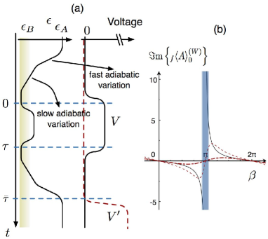
Figure 3: (Color online) (a) An alternative protocol to measure ${}_{f}\langle\hat{A}\rangle_{0}^{(W)}$: shown are $\epsilon$, $V$ and $V^{\prime}$ (notation as in Fig. 2). (b) Imaginary part of the weak value of the spin as a function of $\beta$ for $\Gamma\tau=0$ (full line), $\Gamma\tau=0.1$ (dashed curve) and $\Gamma\tau=1$ (dash-dotted curve). The values of parameters for which the corresponding weak values of spin are obtained with probability $P_{(0,2)}<1\%$ are shadowed.

Here, though the freedom in defining the pre- and post-selected state is reduced: one is restricted to move only within the equatorial plane of the Bloch sphere. The protocol consists in starting with the system in the ground state, $\left|S(0,2)\right\rangle$ (at $\epsilon=\epsilon_{A}$), a slow adiabatic variation (cf. Fig. 1) allows the system to evolve to $\left|\uparrow\downarrow\right\rangle$ at time $t=0$ ($\epsilon=\epsilon_{B}$). The time evolution during the weak measurement pulse is $\mathcal{U}(\tau,0)=\left|S_{g}\right\rangle\left\langle S_{g}\right|+\exp(-i\beta)\left|T_{0}\right\rangle\left\langle T_{0}\right|$, with $\beta=J(\epsilon)\tau$. The evolution from $\tau$ to $\bar{\tau}$ is “slow adiabatic”. The effective post-selected state at time $\tau$ is $|\chi_{f}^{\prime}\left.\right\rangle=\mathcal{U}^{-1}(\bar{\tau},\tau)\left|\chi_{f}\right\rangle$. The weak value of $\mathcal{U}(\tau,0)\hat{A}$ is then ${}_{f}\langle\hat{A}\rangle_{0}^{(W)}=1/2[1-i\tan(\beta/2)]$. The imaginary part of the weak value can then be arbitrary large. Decoherence due to fluctuations of the electromagnetic field is however unavoidable mio . A general scheme to account for the effects of decoherence requires the use of a density matrix, $\rho(\tau)$. In the present protocol decoherence mainly comes from charge fluctuations (fluctuations of $\epsilon$), which commute with the measured operator $\hat{A}$, yielding ${}_{f}\langle\hat{A}\rangle_{0}^{(W)}=\langle\chi_{f}^{\prime}|\rho(\tau)\hat{A}|\chi_{f}^{\prime}\rangle/\langle\chi_{f}^{\prime}|\rho(\tau)|\chi_{f}^{\prime}\rangle$. Here the density matrix is $\rho(\tau)=1/2(\left|S_{g}\right\rangle\left\langle S_{g}\right|+\left|T_{0}\right\rangle\left\langle T_{0}\right|+e^{-i(\beta-i\Gamma\tau)}\left|S_{g}\right\rangle\left\langle T_{0}\right|+e^{+i(\beta+i\Gamma\tau)}\left|T_{0}\right\rangle\left\langle S_{g}\right|)$, where $\Gamma$ is defined by $J(\epsilon)\rightarrow J(\epsilon)+\xi(t)$, with $\langle\xi(t)\xi(t^{\prime})\rangle=2\hbar\Gamma\delta(t-t^{\prime})$ –cf. Fig. 3. In general the strong incoherent limit does not reduce to the standard expectation value of the spin. The presence of coherent oscillations within this protocol Petta et al. (2005), anyway, underlines the possibility to realize this procedure experimentally. The present protocol employs building blocks which have already been tested experimentally (QPCs as charge sensors, spin manipulation in the double dot). Most promising is the experiment setup of Ref. Petta et al. (2005) . The main experimental future challenge here would be a single shot readout, i.e. a quantum mechanical measurement of the state of the dot (without averaging over many repetitions as in ref. [13]). In this context we note that charge sensing by a QPC operated with fast pulses has been recently demonstrated Reilly, Marcus, Hanson, Gossard (2007).

Conclusions.— The protocol outlined above will facilitate the measurement of non-standard (weak) values of spin. The procedure is generalized to include the effect of non-pure states. Further directions may include a systematic study of various mechanisms for decoherence within the weak value scheme and the measurement of two interacting spins (pair of double quantum dots), leading to cross-correlations of weak values.

We are grateful to Y. Aharonov for introducing us to the subject of weak values. We acknowledge useful discussions with Y. Aharonov, L. Vaidman and A. Yacoby on theoretical and experimental aspects of the problem. This work was supported in part by the U.S.-Israel BSF, the DFG project SPP 1285, the Transnational Access Program RITA-CT-2003-506095 and the Minerva Foundation.

Note added.— Upon submission of this manuscript we have noted the paper by Williams and Jordan Williams:2008aa which too discusses weak values in the context of solid state devices.

References

- von Neuman (1932) J. von Neuman, Mathematische Grusndlagen der Quantemechanik (Springler-Verlag, Berlin, 1932).
- Aharonov et al. (1964) Y. Aharonov, P. Bergmann, and J. Lebowitz, Phys. Rev. 134, B1410 (1964).
- Aharonov et al. (1988) Y. Aharonov, D. Z. Albert, and L. Vaidman, Phys. Rev. Lett. 60, 1351 (1988).
- Aharonov and Vaidman (1990) Y. Aharonov and L. Vaidman, Phys. Rev. A 41, 11 (1990).
- 200 (2002) Y. Aharonov, and L. Vaidman, in Time in Quantum Mechanics, J.G. Muga et al. eds., (Springer) 369-412,(2002).
- (6) A. N. Jordan and M. Buttiker, Phys. Rev. Lett. 95, 220401 (2005); W. Hongduo and Y. V. Nazarov, cond-mat/0703344 (2007).
- Neder et al. (2007) I. Neder, M. Heiblum, D. Mahalu, and V. Umansky, Phys. Rev. Lett. 98, 036803 (2007).
- (8) A. Di Lorenzo and Y. V. Nazarov, Phys. Rev. Lett. 93, 046601 (2004); E. Sukhorukov, A. Jordan, S. Gustavsson, R. Leturcq, T. Ihn, and K. Ensslin, Nat Phys 3, 243 (2007), 10.1038/nphys564.
- (9) N. W. M. Ritchie, J. G. Story, and R. G. Hulet, Phys. Rev. Lett. 66, 1107 (1991); A. M. Steinberg, ibid. 74, 2405 (1995); G. J. Pryde, J. L. O’Brien, A. G. White, T. C. Ralph, and H. M. Wiseman, ibid. 94, 220405 (2005).
- Petta et al. (2005) J. R. Petta, A. C. Johnson, J. M. Taylor, E. A. Laird, A. Yacoby, M. D. Lukin, C. M. Marcus, M. P. Hanson, and A. C. Gossard, Science 309, 2180 (2005).
- (11) S. I. Erlingsson, Y. V. Nazarov, and V. I. Fal’ko, Phys. Rev. B 64, 195306 (2001); A. V. Khaetskii, D. Loss, and L. Glazman, Phys. Rev. Lett. 88, 186802 (2002); I. A. Merkulov, A. L. Efros, and M. Rosen, Phys. Rev. B 65 205309 (2002).
- Jordan et al. (2007) A. Jordan, B. Trauzettel, and G. Burkard, arXiv:0706.0180 (2007).
- (13) M. Field, C. G. Smith, M. Pepper, D. A. Ritchie, J. E. F. Frost, G. A. C. Jones, and D. G. Hasko, Phys. Rev. Lett. 70, 1311 (1993); L. DiCarlo, H. J. Lynch, A. C. Johnson, L. I. Childress, K. Crockett, C. M. Marcus, M. P. Hanson, and A. C. Gossard, ibid. 92, 226801 (2004).
- (14) A. N. Korotkov and D. V. Averin, Phys. Rev. B 64, 165310 (2001).
- Averin and Sukhorukov (2005) D. V. Averin and E. V. Sukhorukov, Phys. Rev. Lett. 95, 126803 (2005).
- Johnson et al. (2005) A. C. Johnson, J. R. Petta, J. M. Taylor, A. Yacoby, M. D. Lukin, C. M. Marcus, M. P. Hanson, and A. C. Gossard, Nature 435, 925 (2005).
- (17) F. H. L. Koppens, C. Buizert, K. J. Tielrooij, I. T. Vink, K. C. Nowack, T. Meunier, L. P. Kouwenhoven, and L. M. K. Vandersypen, Nature 442, 766 (2006); E. Laird, C. Barthel, E. Rashba, C. Marcus, M. Hanson, and A. Gossard, cond-mat/0707.0557 (2007).
- (18) G. Burkard, D. Loss, and D. P. DiVincenzo, Phys. Rev. B 59, 2070 (1999); A. Romito and Y. Gefen, ibid. 76, 195318 (2007).
- Reilly, Marcus, Hanson, Gossard (2007) D. J. Reilly, C. M. Marcus, M. P. Hanson, and A. C. Gossard, cond-mat/0707.2946 (2007).
- (20) N. S. Williams, and A. N. Jordan, arXiv:0707.3427 [Phys. Rev. Lett. (to be published)].