$N^{*}$ and $\Delta^{*}$  decays into $N\pi^{0}\pi^{0}$

Abstract

Decays of baryon resonances in the second and the third resonance region into $N\pi^{0}\pi^{0}$ are studied by photoproduction of two neutral pions off protons. Partial decay widths of $N^{*}$ and $\Delta$* resonances decaying into $\Delta(1232)\pi$, $N(\pi\pi)_{S}$, $N(1440)P_{11}$$\pi$, and $N(1520)D_{13}$$\pi$ are determined in a partial wave analysis of this data and of data from other reactions. Several partial decay widths were not known before. Interesting decay patterns are observed which are not even qualitatively reproduced by quark model calculations. In the second resonance region, decays into $\rm\Delta(1232)\pi$ dominate clearly. The $\rm N(\pi\pi)_{S}$-wave provides a significant contribution to the cross section, especially in the third resonance region. The $\rm P_{13}$(1720) properties found here are at clear variance to PDG values.
PACS: 11.80.Et, 13.30.-a, 13.40.-f, 13.60.Le

, , , , , , , , , , , , , , , , , , , , , , , , , , , , , , , , , , , , , , , , , , , , , , ,

The structure of baryons and their excitation spectrum is one of the unsolved issues of strong interaction physics. The ground states and the low–mass excitations evidence the decisive role of SU(3) symmetry and suggest an interpretation of the spectrum in constituent quark models [1, 2, 3]. Baryon decays can be calculated in quark models using harmonic–oscillator wave functions and assuming a $q\bar{q}$ pair creation operator for meson production. A collective string-like model gives a description of the mass spectrum of similar quality [4] and predicts partial decay widths of resonances [5]. A comprehensive review of predictions of baryon masses and decays can be found in [6]. An alternative description of the baryon spectrum may be developed in effective field theories in which baryon resonances are generated dynamically from their decays [7]. At present, the approach is restricted to resonances coupling to octet baryons and pseudoscalar mesons, yet it can possibly be extended to include vector mesons and decuplet baryons [8]. To test the different approaches, detailed information on the spectrum and decays of resonances is needed, including more complex decay modes such as $\Delta\pi$ or $N(\pi\pi)_{\rm S}$, where $(\pi\pi)_{\rm S}$ stands for the $(\pi\pi)$-$S$-wave. The analysis of complex final states requires the use of event-based likelihood fits to fully exploit the sensitivity of the data. In baryon spectroscopy such fits have, to our knowledge, never been performed so far.

In this letter we report on a study of $\Delta\pi$ and other $p2\pi^{0}$ decay modes of baryon resonances belonging to the second and third resonance region. The results are obtained from data on the reaction

$$\gamma p\to p\pi^{0}\pi^{0}\,.$$ (1)

The data were obtained using the tagged photon beam of the ELectron Stretcher Accelerator (ELSA) [9] at the University of Bonn, and the Crystal Barrel detector [10]. A short description of the experiment, data reconstruction and analysis methods can be found in two letters on single $\pi^{0}$ [11] and $\eta$ [12] photoproduction, a more comprehensive one in [13, 14]. The analysis presented here differs only in the final state consisting now of four photons (instead of two or six) and a proton. The data cover the photon energy range from 0.4 to 1.3 GeV.

In the analysis, events due to reaction (1) are selected by requiring five clusters of energy deposits in the Crystal Barrel calorimeter, one of them matching the direction of a charged particle emerging from the liquid H₂ target of 5cm length and hitting a three–layer scintillation fiber (Scifi) detector surrounding the target. The latter cluster is assigned to be a ‘proton’, the other four clusters are treated as photons. Events are also retained when they have four clusters in the calorimeter and a hit in the Scifi which cannot be matched to any of the clusters. The Scifi hit is then treated as ‘proton’, the four hits in the barrel as photons. In a second selection step, the events are subjected to a one–constraint kinematical fit to the $\gamma p\to p4\gamma$ hypothesis imposing energy and momentum conservation and assuming that the interaction took place in the target center. The proton is treated as missing particle, its direction resulting from the fit has to agree with the direction of the detected proton within 20^∘. The $\gamma\gamma$ invariant mass distribution of one photon pair versus the invariant mass distribution of the second photon pair is plotted in Fig. 1a.

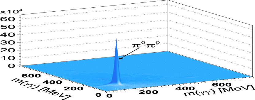
Figure 1: a) $\gamma\gamma$ invariant mass distribution of one photon pair versus the invariant mass distribution of the second photon pair after a kinematical fit to $\gamma p\to p4\gamma$ (6 entries per event). b) Total cross sections for $\gamma p\to p\pi^{0}\pi^{0}$, $\bullet$ this work; ${\tiny\triangle}$: TAPS  [15]; open squares: GRAAL [18]. Solid line: PWA fit, band below the figure: systematic error (see text). Dashed curve: $\Delta^{+}\pi^{0}\to p\pi^{0}\pi^{0}$, dashed-dotted line: $p(\pi^{0}\pi^{0})_{S}$ cross section as derived from the PWA.

A $2\sigma$ cut ($\sigma=8$ MeV/c²) was applied to the two $\pi^{0}$, then the mass of the two $\pi^{0}$ was imposed in a $\gamma p\to p\pi^{0}\pi^{0}\to p\,4\gamma$ three–constraint kinematical fit with a missing proton. Its confidence level had to exceed 10$\%$ and had to be larger than that for a fit to $\gamma p\to p\pi^{0}\eta\to p\,4\gamma$. The final event sample contains 115.600 events. Performing extensive GEANT–based Monte Carlo (MC) simulations, the background was shown to be less than 1$\%$. The acceptance determined from MC simulations vanishes for forward protons leaving the Crystal Barrel through the forward hole, and for protons going backward in the center-of-mass system, having very low laboratory momenta. The overall acceptance depends on the contributing physics amplitudes which are determined by a partial wave analysis (PWA) described below. MC events distributed according to the PWA solution were used to determine the correct acceptance. This MC data sample undergoes the same analysis chain as real data.

We first discuss the main features of the data. Fig. 1b shows the total cross section for $2\pi^{0}$ photoproduction together with the $\Delta\pi$ and $p(\pi\pi)_{S}$ excitation functions. Two peaks due to the second and third resonance region are immediately identified. Our data points are given by black dots, the bars represent the statistical errors. The systematic error due to the acceptance correction is determined by the spread of results obtained from different PWA solutions. A second systematic error is due to uncertainties in the reconstruction [13]. These errors are added quadratically to determine the total systematic error shown as a band below the cross section. This error does not contain the normalization uncertainty of $\pm 5\%$ [13].

The general consistency between our data and those from A2-TAPS [15] (superseding in statistics earlier MAMI data [16, 17]) and GRAAL [18] is good (see Fig. 1b). In the low–energy region, our data show a shoulder which is less pronounced in the A2-TAPS data (see [15]). The recent A2-GDH measurements [19] fall in between these two results. The DAPHNE data exceed our cross section significantly [20]. At larger energies, the GRAAL data fall off with energy faster than our data. Data taken at higher energies covering the photon energy range from 0.8 to 3 GeV yield a cross section [21] which is compatible in the overlap region with the results presented here. All 3 experiments do not cover the full solid angle. In this analysis and in the analysis of the A2-TAPS collaboration, the cross section is extrapolated into “blind” detector regions using the result of the partial wave analysis. The GRAAL collaboration simulates $\gamma p\to\Delta^{+}\pi^{0}$ and $\gamma p\to p\pi^{0}\pi^{0}$ to account for the acceptance.

Fig. 2a,b) shows the $p\pi^{0}$ and $\pi^{0}\pi^{0}$ invariant mass distribution for reaction (1) after a 1550–1800 MeV/c² cut in the $p\pi^{0}\pi^{0}$ mass. Also shown are some angular distributions. The data and their errors are represented by crosses, the lines give the result of the fits described below. The $p\pi^{0}$ mass distribution reveals the role of the $\Delta$ as contributing isobar. The $\pi^{0}\pi^{0}$ mass distribution does not show any significant structure. While $2\pi$ decays of resonances belonging to the 2^nd resonance region are completely dominated by the $\Delta\pi$ isobar as intermediate state, the two-pion S-wave provides a significant decay fraction in the 3^rd resonance region.

The partial wave analysis uses an event–based maximum likelihood fit.

Figure 2: Mass and angular distributions for $\gamma p\to p\pi^{0}\pi^{0}$ after a 1550–1800 MeV/c² cut on $M_{p\pi^{0}\pi^{0}}$. a: $p\pi^{0}$, b: $\pi^{0}\pi^{0}$ invariant mass. In c)–f) $\cos\theta$ distributions are shown. In (c), $\theta$ is the angle of a $\pi^{0}$ with respect to the incoming photon in the center–of–mass–system (cms); in (d), the cms angle of the proton with respect to the photon is shown; in (e), the angle between two pions in the $\pi^{0}p$ rest frame; in (f) the angle between $\pi^{0}$ and $p$ in the $\pi^{0}\pi^{0}$ rest frame. Data are represented by crosses, the fit as solid line, the thin line in a,b) shows the phase space distribution. Dashed: $\Delta^{+}\pi^{0}\to p\pi^{0}\pi^{0}$, dotted: $p(\pi^{0}\pi^{0})_{S}$ contribution. The distributions are not corrected for acceptance to allow a fair comparison of the fit with the data without introducing any model dependence by extrapolating e.g. over acceptance holes. Differential cross sections will be given elsewhere.

To constrain the analysis, not only the data on reaction (1) were used in the fit but also data on $\gamma p\to p\pi^{0}$ [11, 22, 23, 24, 25, 26, 27, 28] including differential cross sections, beam and target asymmetry, and recoil polarization, further data on $\gamma p\to p\pi^{0}\pi^{0}$ [18, 19], $\gamma p\to p\eta$ [12, 29, 30, 31], and data on $\gamma p\to K\Lambda$, and $K\Sigma$ [32, 33, 34, 35, 36, 37, 38]. The SAID $\pi N$ partial-wave elastic scattering amplitudes [39] are used to constrain the K-matrices for the $S_{11}$, $P_{11}$, $P_{13}$, $P_{33}$, $D_{33}$ partial waves. Details of the fitting procedure and on the $\chi^{2}$ contributions of the different reactions are given in [40]. As examples, we show in Fig. 4 the beam asymmetry $\Sigma$ [18] and in Fig. 4 the helicity dependence of the reaction $\gamma p\to p\pi^{0}\pi^{0}$ [19]. Inclusion of the beam asymmetry had an impact on the size of couplings but did not lead to significant changes of the pole positions. The helicity dependence was correctly predicted; correspondingly, its inclusion had no effect on the final solution.

Figure 3: The beam asymmetry $\Sigma$ for the reaction $\gamma p\to p\pi^{0}\pi^{0}$ as a function of the proton or $\pi^{0}$ direction with respect to the beam axis, and as a function of the $\pi^{0}\pi^{0}$ and $p\pi^{0}$ invariant mass [18]. The solid line represents the PWA fit. The numbers given in the figures indicate the photon energy bin.

Figure 4: Helicity dependence of the reaction $\gamma p\to p\pi^{0}\pi^{0}$ [19]. The lines represent the result of the PWA fit.

Particularly useful were the Crystal Ball data on the charge exchange reaction $\pi^{-}p\to n\pi^{0}\pi^{0}$ [41]. Even though limited to masses below 1.525 GeV/c², the data provided also valuable constraints for the third resonance region due to their long low–energy tails. The log likelihoods of the different data sets are added with some weights varying from 1 to up to 30 [40]. The weights are chosen to force the fits to describe low-statistics data with reasonable accuracy even on the expense of a worse description of high-statistics data, where large $\chi^{2}$ contributions can be the result of small deficiencies due to model imperfections. The data on $2\pi^{0}$ photoproduction enter with a weight 4. Moderate changes in the weights lead to changes in the results which are covered by the quoted errors.

We started the analysis from the solution given in [42, 43] and found good compatibility. The new $p\pi^{0}\pi^{0}$ data provides information on the N$\pi\pi$ decay modes, without inducing the need to change masses or widths of the contributing resonances (from [42, 43]) beyond their respective errors, even though all parameters were allowed to adjust again. The quality of the fits of the previous data did not worsen significantly due to the constraints by the new $p\pi^{0}\pi^{0}$-data.

The dynamical amplitudes comprise resonances and background terms due to Born graphs and $t$– and $u$–channel exchanges. Angular distributions are calculated using relativistic operators [44]. Relations between cross sections and resonance partial widths are given in [45]. Most partial waves are described by multi–channel Breit-Wigner amplitudes with an energy dependent width (in the form suggested by Flatté [46]). Partial widths are calculated at the position of the Breit-Wigner mass. For the K-matrix parameterizations the Breit-Wigner parameters are determined in the following way. First, the couplings are calculated as T-matrix pole residues, then the imaginary part of the Breit-Wigner denominator is parameterized as a sum of these couplings squared, multiplied by the corresponding phase volumes and scaled by a common factor. This factor as well as the Breit-Wigner mass are chosen as to reproduce the amplitude pole position on the Rieman sheet closest to the physical region. The Breit-Wigner parameters of the $S_{11}$-resonances are determined without taking into account the $\Delta\pi$-width to obtain results which can be compared with the Particle Data Group (PDG) values [47].

Table 1 summarizes the results of our fits. In the absence of double-polarization data, there is no unique solution. We have studied a large variety of solutions and estimated the errors in the Table from the range of values found for different solutions giving an acceptable description of the data. Most results agree, within their respective errors, reasonably well with previous findings. The errors quoted are estimated from the variance of results of a large number of fits which provide an adequate description of the data. Several partial decay widths for baryon decays into $N\pi\pi$ were not known before. For widths known from previous analyses, good compatibility is found. The helicity amplitudes quoted in the table are calculated at the position of the resonance pole. Hence they acquire a phase. As long as the phase is small, the comparison with PDG values is still meaningful. We now discuss a few partial waves.

The $P_{13}$ wave is described by a three-pole multi-channel K-matrix which we interpret as $N(1720)P_{13}$, $N(1900)P_{13}$, and $N(2200)P_{13}$. The $N(1900)P_{13}$ resonance is required [48] due to the inclusion of the CLAS spin transfer measurements in hyperon photoproduction [37]. The $N(2200)P_{13}$ was already needed to fit single-pion photoproduction [42].

Table 1: Properties of the resonances contributing to the $\gamma p\to\pi^{0}\pi^{0}p$ cross section. The masses and widths are given in MeV, the branching ratios $\mathcal{B}$ in % and helicity couplings in GeV^-1/2. The helicity couplings and phases were calculated as residues in the pole position which is denoted as ‘Mass’ and ‘$\Gamma_{tot}$’. The method for calculation of Breit-Wigner parameters is described in the text.

	$N(1535)S_{11}$	$N(1650)S_{11}$	$N(1520)D_{13}$	$N(1700)D_{13}$	$N(1675)D_{15}$	$N(1720)P_{13}$	$N(1680)F_{15}$	$\Delta(1620)S_{31}$	$\Delta(1700)D_{33}$
Mass	1508${}^{+10}_{-30}$	1645$\pm$15	1509$\pm$7	1710$\pm$15	1639$\pm$10	1630$\pm$90	1674$\pm$5	1615$\pm$25	1610$\pm$35
rrrrr PDG	1495–1515	1640–1680	1505–1515	1630–1730	1655–1665	1660–1690	1665–1675	1580–1620	1620–1700
$\rm\Gamma_{tot}$	165$\pm$15	187$\pm$20	113$\pm$12	155$\pm$25	180$\pm$20	460$\pm$80	95$\pm$10	180$\pm$35	320$\pm$60
rrrrr PDG	90–250	150–170	110–120	50–150	125–155	115–275	105–135	100–130	150–250
MBW	1548$\pm$15	1655$\pm$15	1520$\pm$10	1740$\pm$20	1678$\pm$15	1790$\pm$100	1684$\pm$8	1650$\pm$25	1770$\pm$40
rrrrr PDG	1520–1555	1640–1680	1515–1530	1650–1750	1670–1685	1700–1750	1675–1690	1615–1675	1670–1770
$\Gamma^{BW}_{tot}$	170$\pm$20	180$\pm$20	125$\pm$15	180$\pm$30	220$\pm$25	690$\pm$100	105$\pm$8	250$\pm$60	630$\pm$150
rrrrr PDG	100–200	145–190	110–135	50–150	140–180	150–300	120–140	120–180	200–400
$A_{1/2}$	0.086$\pm$0.025	0.095$\pm$0.025	0.007$\pm$0.015	0.020$\pm$0.016	0.025$\pm$0.01	0.15$\pm$0.08	-(0.012$\pm$0.008)	0.13$\pm$0.05	0.125$\pm$0.030
rrrrr phase	$(20\pm 15)^{\circ}$	$(25\pm 20)^{\circ}$	$-$	$-(4\pm 5)^{\circ}$	$-(7\pm 5)^{\circ}$	$-(0\pm 25)^{\circ}$	$-(40\pm 15)^{\circ}$	$-(8\pm 5)^{\circ}$	$-(15\pm 10)^{\circ}$
rrrrr PDG	$(0.090\pm 0.030)$	$(0.053\pm 0.016)$	-$(0.024\pm 0.009)$	$-(0.018\pm 0.013)$	0.019$\pm$0.008	0.018$\pm$0.030	$-(0.015\pm 0.006)$	$0.027\pm 0.011$	$(0.104\pm 0.015)$
$A_{3/2}$			0.137$\pm$0.012	0.075$\pm$0.030	0.044$\pm$0.012	0.12$\pm$0.08	0.120$\pm$0.015		0.150$\pm$0.060
rrrrr phase			$-(5\pm 5)^{\circ}$	$-(6\pm 8)^{\circ}$	$-(7\pm 5)^{\circ}$	$-(20\pm 40)^{\circ}$	$-(5\pm 5)^{\circ}$		$-(15\pm 10)^{\circ}$
rrrrr PDG			$0.166\pm 0.005$	$-(0.002\pm 0.024)$	0.015$\pm$0.009	-(0.019$\pm$0.020)	0.133$\pm$0.012		0.085$\pm$0.022
$\rm\mathcal{B}_{miss}$	-	-	13$\pm$5 %	20$\pm$15 %	20$\pm$8 %	-	2$\pm$2 %	10$\pm$7 %	15$\pm$10 %
rrrrrPDG($N\rho$)	$<4$ %	4–12 %	15–25 %	$<35$ %	$<$1–3 %	70–85 %	3–15 %	7–25 %	30–55
$\rm\mathcal{B}_{\pi N}$	37$\pm$9 %	70$\pm$15 %	58$\pm$8 %	8${}^{+8}_{-4}$ %	30$\pm$8 %	9$\pm$6 %	72$\pm$15 %	22$\pm$12 %	15$\pm$8 %
rrrrr PDG	35–55 %	55–90 %	50–60 %	5–15 %	40–50 %	10–20 %	60–70 %	10–30 %	10–20 %
$\rm\mathcal{B}_{\eta N}$	40$\pm$10 %	15$\pm$6 %	0.2$\pm$0.1 %	10$\pm$5 %	3$\pm$3 %	10$\pm$7 %	$<1$ %	-	-
rrrrr PDG	30–55 %	3–10 %	0.23$\pm$0.04 %	0$\pm$1 %	0$\pm$1 %	4$\pm$1 %	0$\pm$1 %
$\rm N\sigma$	-	-	$<4$ %	18$\pm$12 %	10$\pm$5	3$\pm$3 %	11$\pm$5 %	-
rrrrr PDG		$<4$ %	$<8$ %			-	5–20 %
$\rm\mathcal{B}_{K\Lambda}$	-	5$\pm$5 %	-	1$\pm$1 %	3$\pm$3 %	12$\pm$9 %	$<1$ %		-
$\rm\mathcal{B}_{K\Sigma}$	-	-	-	$<1$ %	$<1$ %	$<1$ %	$<1$ %
$\rm\mathcal{B}_{\Delta\pi(L\!<\!J)}$			12$\pm$4 %	10$\pm$5 %	24$\pm$8 %	38$\pm$20 %	8$\pm$3 %	48$\pm$25 %
$L<J$  PDG			5–12 %			-	6–14 %	30–60 %
									70$\pm$20 %
									30–60 %
$\rm\mathcal{B}_{\Delta\pi(L\!>\!J)}$	23$\pm$8 %	10$\pm$5 %	14$\pm$5 %	20$\pm$11 %	$<3$ %	7$\pm$8 %	4$\pm$3 %
$L>J$  PDG	$<$1 %		10-14 %			-	$<2$ %
$\rm\mathcal{B}_{P_{11}\pi}$			2$\pm$2 %	14$\pm$8 %	$<3$ %	-	-	19$\pm$12 %	$<5$ %
$\rm\mathcal{B}_{D_{13}\pi}$			-	-	4$\pm$4 %	24$\pm$20 %	-	-	$<3$ %

Here, only the $N(1720)P_{13}$ resonance is discussed; for further information, see [48]. The $N(1720)P_{13}$ resonance is the only resonance with properties which are clearly at variance with PDG values. The central value for its total width $\Gamma_{tot}^{BW}$ is 400 to 500 MeV compared to the 200 MeV estimate of the PDG. However, Manley et al. [50] find $(380\pm 180)$ MeV/c². Its strongest decay mode is found to be $\Delta\pi$, not reported in [47]. We find a rather small missing width of (6$\pm$1)% of the total width while the PDG assigns $70-85\%$ to the $N\rho$-decay mode. A similar discrepancy was observed in electro-production of two charged pions [51], and interpreted either as evidence for a new – rather narrow – $P_{13}$-state or as a wrong PDG $N\rho$-decay width. In agreement with [52], we find a large branching ratio for $N(1720)P_{13}$$\to N\eta$ while most analyses ascribe the $N\eta$ intensity in this mass region to $N(1710)P_{11}$.

The $P_{33}$ wave is represented by a two-pole two-channel K-matrix. The low energy part of pion photoproduction is described by the $\Delta(1232)$ state even though non-resonant contributions were needed to get a good fit. The quality of the description of the elastic amplitude improved dramatically by introduction of a second pole. The first K-matrix pole has $1231\pm 4$ MeV/c² mass and helicity couplings $a_{1/2}=-0.125\pm 0.008$ and $a_{3/2}=-0.267\pm 0.010$. The pole position in the complex energy plane was found to be $M=1205\pm 4$ MeV/c² and $2\times Im=92\pm 10$ MeV/c². The second K-matrix pole was not very stable and varied between 1650 and 1800 MeV/c². The T-matrix pole showed better stability, and gave $M=1550\pm 40$ MeV/c² and $\Gamma=290\pm 60$ MeV/c². This can be compared to the PDG ranges, $M=1550-1700$ MeV/c² and $\Gamma=250-450$ MeV/c².

The two $S_{11}$ resonances (Table 1) are treated as coupled–channel $5\otimes 5$ K-matrix including $N\pi$, $N\eta$, $K\Lambda$, $K\Sigma$, and $\Delta\pi$ as channels. The $N\sigma$ or the $N\rho$ decay mode were added as 6^th channel for part of the fits. The first K-matrix pole varied over a wide range in different fits, from 1100 to 1480 MeV/c². The physical amplitude (T-matrix) exhibited, however, a stable pole at M_pole=1508${}^{+10}_{-30}$ -i(83$\pm$8) MeV/c², in good agreement with PDG. This pole position is very close to the $\eta N$ threshold. In some fits the pole moved under the $\eta N$ cut; in that case the closest physical region for this pole is the $\eta N$ threshold. No other pole around 1500 MeV/c² close to the physical region was then found on any other sheet. The second K-matrix pole always converged to $1715\pm 30$ MeV/c² resulting in a T-matrix pole as given in Table 1. Introduction of an additional pole did not lead to a significant improvement in the fit.

The $P_{11}$ partial wave is largely non-resonant. Two $P_{11}$ resonances were needed to describe this partial wave, the Roper resonance and a second one situated in the region 1.84-1.89 GeV/c². Detailed information on the $P_{11}$-partial wave is given in an accompanying letter [15].

The reaction $\gamma p\to p\pi^{0}\pi^{0}$ gives access to the isobar decomposition of proton-plus-two-pion decays of baryon resonances. The important intermediate states are $\Delta(1232)\pi$, $N(\pi\pi)_{S}$, $N(1440)P_{11}$$\pi$ and $N(1520)D_{13}$$\pi$ (see Table 1). The $N(\pi\pi)_{\rm S}$-wave contributes significantly in the $3^{\rm rd}$ resonance region in which the three states $N(1700)D_{13}$ , $N(1675)D_{15}$ , and $N(1680)F_{15}$ are shown to have non-negligible couplings to $N(\pi\pi)_{\rm S}$. The $N(1700)D_{13}$ and $\Delta(1620)S_{31}$ decay with a significant fraction into $P_{11}(1440)\pi$, a decay mode which has not yet been reported for these resonances. Naively, this decay mode is expected to be suppressed by either the orbital angular momentum barrier and/or by the smallness of the available phase space.

New and unexpected results were obtained for decays into $\Delta\pi$. The $\Delta\pi$-contribution clearly dominates the cross section, especially at lower energies (Fig.1). An interesting pattern of partial decays of resonances into $\Delta\pi$ is observed which is neither expected by phase space arguments nor by quark model calculations. $D_{13}$-decays into $\Delta\pi_{(S-wave)}$ are allowed by all selection rules but are observed to be weaker than naively expected. The $N(1520)D_{13}$ decays into $\Delta\pi$ in D–wave with about the same strength as in S-wave even though the orbital angular momentum barrier should suppress D-wave decays for such small momenta ($\sim 250$ MeV/c). The $N(1700)D_{13}$ $\Delta\pi_{(S-wave)}$-decay is observed to be weaker than $\Delta\pi_{(D-wave)}$. For both $D_{13}$-states, the $\Delta\pi_{(S-wave)}$ seems to be suppressed dynamically. For other resonances, like $N(1675)D_{15}$, and $N(1680)F_{15}$  the lower orbital momentum partial wave is preferred. The $N(1535)S_{11}$ and $N(1650)S_{11}$ resonances show sizable couplings to $\Delta\pi$, even though $L=2$ is required. The $\Delta(1700)D_{33}$ state decays dominantly into $\Delta\pi$. Unfortunately no statement on the dominance of the S- or D-wave decay of the $\Delta(1700)D_{33}$ can be made. Two distinct solutions have been found; for one of them the S-wave, for another one the D-wave, dominates clearly. The forthcoming double polarisation experiments will help to resolve this ambiguity.

The results on the decays can be compared to model calculations by Capstick and Roberts (A); Koniuk and Isgur (B); Stassart and Stancu (C); Bijker, Le Yaouanc, Oliver, Pène and Raynal (D), and Iachello and Leviatan (E); (numbers and references can be found in [6], Table VI and VII). A quality factor (mean fractional deviation) can be defined by the fractional difference between prediction $x_{i}$ and experimental result $y_{i}$ as $q_{i}=4(|x_{i}|-|y_{i}|)^{2}/(|x_{i}|+|y_{i}|)^{2}$. The $x_{i},y_{i}$ are proportional to the amplitude for a decay, they are normalized to give $x_{i}^{2}=\Gamma_{i}$. The $x_{i}$ carry a signature which is not given for all calculations. To enable a meaningful comparison, only absolute values are considered in the comparison. The rms value of the 14 $q_{i}$ values is calculated for each model to define a ‘model’ quality.

$$\scriptsize q_{A}=0.271;\quad\scriptsize q_{B}=0.247;\quad\scriptsize q_{C}=0.328;\quad\scriptsize q_{D}=0.222;\quad\scriptsize q_{E}=0.219\,.$$ (2)

The model (A) is the only model which predicts the correct signature in 13 out of the 14 cases. This achievement is not taken into account in the comparison (2). The (formally) most successful model describes baryons in terms of rotations and vibrations of strings and their algebraic relations [5].

Summarizing, we have presented new data on the reaction $\gamma p\to p\pi^{0}\pi^{0}$. The partial wave analysis reveals various contributions to the 2^nd and 3^rd resonance region. Most masses and widths determined here are in reasonable agreement with known resonances. Yet, several $p2\pi^{0}$-decay widths contradict expectation. An interesting pattern of partial decays of resonances into $\Delta\pi$ is observed which was not predicted by quark model calculations. Several $p2\pi$-partial widths for baryon resonances in the 2^nd and 3^rd resonance region and the excitation functions for $\gamma p\to\Delta\pi$ and $\gamma p\to N(\pi\pi)_{s}$ have been determined for the first time.

We would like to thank the technical staff of the ELSA machine groups and of all the participating institutions of their invaluable contributions to the success of the experiment. We acknowledge financial support from the Deutsche Forschungsgemeinschaft (DFG) within the SFB/TR16 and from the Schweizerische Nationalfond. The collaboration with St. Petersburg received funds from DFG and RFBR. U.Thoma thanks for an Emmy Noether grant from the DFG. A.V. Sarantsev acknowledges support from RSSF. This work comprises part of the thesis of M. Fuchs.

References

- [1] S. Capstick and N. Isgur, Phys. Rev. D 34 (1986) 2809.
- [2] L. Y. Glozman et al., Phys. Rev. D 58 (1998) 094030.
- [3] U. Löring et al., Eur. Phys. J. A 10 (2001) 395, 447.
- [4] R. Bijker, F. Iachello and A. Leviatan, Annals Phys. 236 (1994) 69.
- [5] R. Bijker, F. Iachello and A. Leviatan, Phys. Rev. D 55 (1997) 2862.
- [6] S. Capstick and W. Roberts, Prog. Part. Nucl. Phys. 45 (2000) S241.
- [7] E. Oset et al., Int. J. Mod. Phys. A 20 (2005) 1619.
- [8] M. F. M. Lutz and E. E. Kolomeitsev, Nucl. Phys. A 755 (2005) 29.
- [9] W. Hillert, Eur. Phys. J. A 28S1 (2006) 139.
- [10] E. Aker et al., Nucl. Instrum. Meth. A 321 (1992) 69.
- [11] O. Bartholomy et al., Phys. Rev. Lett. 94 (2005) 012003.
- [12] V. Crede et al., Phys. Rev. Lett. 94 (2005) 012004.
- [13] H. van Pee et al., Eur. Phys. J. A 31 (2007) 61.
- [14] O. Bartholomy et al., Eur. Phys. J. A 33 (2007) 133.
- [15] A. Sarantsev et al., “New results on the Roper resonance and the partial wave,” arXiv:0707.3591.
- [16] F. Harter et al., Phys. Lett. B 401 (1997) 229.
- [17] M. Wolf et al., Eur. Phys. J. A 9 (2000) 5.
- [18] Y. Assafiri et al., Phys. Rev. Lett. 90 (2003) 222001.
- [19] J. Ahrens et al., Phys. Lett. B 624 (2005) 173.
- [20] A. Braghieri et al., Phys. Lett. B 363 (1995) 46.
- [21] M. Fuchs, PhD thesis, Bonn, 2005.
- [22] A. A. Belyaev et al., Nucl. Phys. B 213 (1983) 201.
- [23] R. Beck et al., Phys. Rev. Lett. 78 (1997) 606.
- [24] D. Rebreyend et al.,Nucl. Phys. A 663 (2000) 436.
- [25] K. H. Althoff et al., Z. Phys. C 18 (1983) 199.
- [26] E. J. Durwen, BONN-IR-80-7 (1980).
- [27] K. Buechler et al., Nucl. Phys. A 570 (1994) 580.
- [28] O. Bartalini et al., Eur. Phys. J. A 26 (2005) 399.
- [29] B. Krusche et al., Phys. Rev. Lett. 74 (1995) 3736.
- [30] J. Ajaka et al., Phys. Rev. Lett. 81 (1998) 1797.
- [31] O. Bartalini et al., Eur. Phys. J. A 33 (2007) 169.
- [32] K. H. Glander et al., Eur. Phys. J. A 19 (2004) 251.
- [33] J. W. C. McNabb et al., Phys. Rev. C 69 (2004) 042201.
- [34] R. G. T. Zegers et al., Phys. Rev. Lett. 91 (2003) 092001.
- [35] R. Lawall et al., Eur. Phys. J. A 24 (2005) 275.
- [36] R. Bradford et al., Phys. Rev. C 73 (2006) 035202.
- [37] R. Bradford et al., Phys. Rev. C 75 (2007) 035205.
- [38] A. Lleres et al., Eur. Phys. J. A 31 (2007) 79.
- [39] R. A. Arndt et al., Phys. Rev. C 74 (2006) 045205.
- [40] A. V. Anisovich et al., “Baryon resonances and polarization transfer in hyperon photoproduction,” arXiv:0707.3596.
- [41] S. Prakhov et al., Phys. Rev. C 69 (2004) 045202.
- [42] A. V. Anisovich et al., Eur. Phys. J. A 25 (2005) 427.
- [43] A. V. Sarantsev et al., Eur. Phys. J. A 25 (2005) 441.
- [44] A.V. Anisovich et al., Eur. Phys. J. A 24 (2005) 111.
- [45] A. V. Anisovich and A. V. Sarantsev, Eur. Phys. J. A 30 (2006) 427.
- [46] S. M. Flatté, Phys. Lett. B 63 (1976) 224.
- [47] W. M. Yao et al. [Particle Data Group], J. Phys. G 33 (2006) 1.
- [48] V. A. Nikonov et al., “Further evidence for from photoproduction of hyperons”, arXiv:0707.3600.
- [49] T.P. Vrana, S.A. Dytman and T.S.H. Lee, Phys. Rept. 328 (2000) 181.
- [50] D.M. Manley, E.M. Saleski, Phys. Rev. D 45 (1992) 4002.
- [51] M. Ripani et al., Phys. Rev. Lett. 91 (2003) 022002.
- [52] I.G. Aznauryan, Phys. Rev. C 68 (2003) 065204.