Chiral Plaquette Polaron Theory of Cuprate Superconductivity

Abstract

Ab-initio density functional calculations on explicitly doped La_2-xSr_xCuO₄ find doping creates localized holes in out-of-plane orbitals. A model for cuprate superconductivity is developed based on the assumption that doping leads to the formation of holes on a four-site Cu plaquette composed of the out-of-plane A₁ orbitals apical O $p_{z}$, planar Cu d${}_{3z^{2}-r^{2}}$, and planar O $p_{\sigma}$. This is in contrast to the assumption of hole doping into planar Cu $d_{x^{2}-y^{2}}$ and O $p_{\sigma}$ orbitals as in the t-J model. Allowing these holes to interact with the $d^{9}$ spin background leads to chiral polarons with either a clockwise or anti-clockwise charge current. When the polaron plaquettes percolate through the crystal at $x\approx 0.05$ for La_2-xSr_xCuO₄, a Cu $d_{x^{2}-y^{2}}$ and planar O $p_{\sigma}$ band is formed. The computed percolation doping of $x\approx 0.05$ equals the observed transition to the “metallic” and superconducting phase for La_2-xSr_xCuO₄. Spin exchange Coulomb repulsion with chiral polarons leads to D-wave superconducting pairing. The equivalent of the Debye energy in phonon superconductivity is the maximum energy separation between a chiral polaron and its time-reversed partner. This energy separation is on the order of the antiferromagnetic spin coupling energy, $J_{dd}\sim 0.1$ eV, suggesting a higher critical temperature. An additive skew-scattering contribution to the Hall effect is induced by chiral polarons and leads to a temperature dependent Hall effect that fits the measured values for La_2-xSr_xCuO₄. The integrated imaginary susceptibility, observed by neutron spin scattering, satisfies $\omega/T$ scaling due to chirality and spin-flip scattering of polarons along with a uniform distribution of polaron energy splittings. The derived functional form is compatible with experiments. The static spin structure factor for chiral spin coupling of the polarons to the undoped antiferromagnetic Cu $d^{9}$ spins is computed for classical spins on large two dimensional lattices and is found to be incommensurate with a separation distance from $(\pi/a,\pi/a)$ given by $\delta Q\approx(2\pi/a)x$ where $x$ is the doping. When the perturbed $x^{2}-y^{2}$ band energy in mean-field is included, incommensurability along the Cu$-$O bond direction is favored. A resistivity $\sim T^{\mu+1}$ arises when the polaron energy separation density is of the form $\sim\Delta^{\mu}$ due to Coulomb scattering of the $x^{2}-y^{2}$ band with polarons. A uniform density leads to linear resistivity. The coupling of the $x^{2}-y^{2}$ band to the undoped Cu $d^{9}$ spins leads to the angle resolved photoemission pseudogap and its qualitative doping and temperature dependence. The chiral plaquette polaron leads to an explanation of the evolution of the bi-layer splitting in Bi-2212.

I Introduction

It is generally assumed that the relevant orbitals for understanding high temperature cuprate superconductivity arise from holes on planar Cu $d_{x^{2}-y^{2}}$ and O $p_{\sigma}$ orbitals. The t-J modelanderson_tj and its generalization to the three band Hubbard modelemery are believed to be the correct Hamiltonians for understanding these materials. Extensive work since the original discoverybednorz_muller has not led to a complete understanding of the properties of the cuprates, despite the rich physics contained in such a simple Hamiltonian.

In this paper, we assume doping creates polarons composed of apical O $p_{z}$ hybridized with Cu $d_{3z^{2}-r^{2}}$ and planar O $p_{\sigma}$ that form localized chiral states in the vicinity of the dopant (Sr in La_2-xSr_xCuO₄, for example). The polaron orbital is spread over the 4-site Cu plaquette near the Sr and is stabilized in a chiral state due to its interaction with the antiferromagnetic $d^{9}$ spins on the undoped Cu sites. This is similar to prior work siggia1 ; siggia2 ; siggia3 ; zee1 ; gooding1 suggesting chiral spins states arise from doping except, in our case, the polaron is formed from out-of-plane orbitals.

As the doping is increased, the chiral polarons eventually percolate through the crystal. We assume a Cu $d_{x^{2}-y^{2}}$ and O $p_{\sigma}$ delocalized band is formed in the percolating swath. This leads to our Hamiltonian of a delocalized Cu $d_{x^{2}-y^{2}}$ band interacting with chiral plaquette polarons and localized $d^{9}$ antiferromagnetic spins on the undoped Cu sites.

For low dopings, momentum k is not a good quantum number because the $x^{2}-y^{2}$/$p_{\sigma}$ band is formed on the percolating swath. This leads to broadening observed in angle-resolved photoemission (ARPES) measurements. As the doping is increased, k becomes a better quantum number.

With increasing doping the 4-site chiral polarons crowd together in the crystal and several changes occur. First, the apical O and single Cu closest to Sr is doped with $p_{z}$ instead of the four Cu’s of the plaquette.ub3lyp_dope Second, the reduction of undoped $d^{9}$ spins decreases the energy difference between a polaron state and its time-reversed partner. Third, the number of $x^{2}-y^{2}$/$p_{\sigma}$ band electrons increases.

In our model, the superconducting d-wave pairing is due to the Coulomb spin exchange interaction of the $x^{2}-y^{2}$ band with chiral polarons where the Debye energy in phonon superconductors is replaced by the maximum energy difference of a polaron with its time-reversed partner (the polaron with flipped chirality and spin). This leads to an overdoped phase where superconductivity is suppressed.

Calculations in this paper of the doping values of La_2-xSr_xCuO₄ and YBa₂Cu₃O_6+δ for percolation of polaron plaquettes and the formation of an $x^{2}-y^{2}$ band are $x\approx 0.05$ and $\delta\approx 0.36$. Percolation of single doped apical O $p_{z}$ and Cu $z^{2}$ described above is $x\approx 0.20$. These numbers are close to known phase transitions in La_2-xSr_xCuO₄birgeneau_rmp ; cava_ortho ($x\approx 0.05$ for the spin-glass to superconducting transition and $x\approx 0.20$ for the orthorhombic to tetragonal transition) and YBa₂Cu₃O_6+δybco_af_sc ($\delta\approx 0.35$ for the antiferromagnetic to superconducting transition).

Chiral polarons couple to the Cu $d^{9}$ spins on the undoped sites and distort the antiferromagnetic order leading to incommensurate magnetic neutron scattering peaks. The charge current of the polaron induces a chiral coupling of the form $\pm J_{ch}[{\mathbf{S}_{z}\cdot(\mathbf{S}_{d1}\times\mathbf{S}_{d2})}]$ zee1 ; gooding1 ; gooding_birgeneau where $\mathbf{S}_{z}$ is the polaron spin and the subscripts $d1$ and $d2$ represent Cu $x^{2}-y^{2}$ spins at adjacent sites. The sign of the interaction is determined by the chirality of the polaron. This term is in addition to an antiferromagnetic coupling between the polaron spin and a neighboring $d^{9}$ spin, $J_{dz}$, and the $d^{9}-d^{9}$ spin coupling, $J_{dd}$.

We have performed energy minimizations on large lattices of classical spins doped with chiral plaquette polarons over a range of coupling parameters to compute the static spin structure factor. These calculations are similar to previous computations of the correlation length and incommensurability due to chiral plaquettesgooding_birgeneau using the Grempel algorithmgrempel to search for a global minimum. A neutron incommensurability peak consistently appears on a circle in k-space centered at $(\pi/a,\pi/a)$ with radius $\approx(2\pi/a)x$. This result is missing the kinetic energy perturbation of the $d_{x^{2}-y^{2}}$ band. Computing this contribution in mean field selects the incommensurate peaks along the Cu-O bond directions in accord with experiments. birgeneau_rmp ; incommen_metal1 ; incommen_metal2 ; incommen_metal3

If the energy difference between a chiral state and its time-reversed partner, where the spin and chirality are flipped, is uniformly distributed over an energy range larger than the temperature, then the dynamical magnetic response of the polarons satisfies $\omega/T$ scaling. neutron_scaling1 ; neutron_scaling2 ; neutron_scaling3 ; neutron_scaling4 ; neutron_scaling5 ; neutron_scaling6 ; neutron_scaling7 ; birgeneau_rmp Since the polarons are randomly distributed throughout the crystal with different undoped $d^{9}$ environments, the probability distribution of the energy separation of these states may be approximately uniform.

There are four possible orbital state symmetries for a polaron delocalized over a four Cu plaquette. They are $S$, $D_{xy}$, and $P_{x^{\prime}}\pm iP_{y^{\prime}}$, where the last two states are chiral. $x^{\prime}$, $y^{\prime}$ refer to axes along the diagonals. Coulomb scattering of Cu $x^{2}-y^{2}$ band electrons with polarons leads to a linear resistivity in the case of a uniform energy distribution of the energies of the four polaron states. This may be uniform for the same reasons discussed above for neutron scaling. Any non-uniformity of the energy distribution spectrum makes the resistivity non-linear.

Spin exchange Coulomb scattering of an $x^{2}-y^{2}$ Cooper pair $(\mathbf{k}\uparrow,\mathbf{-k}\downarrow)$ with a chiral polaron $P_{x^{\prime}}\pm iP_{y^{\prime}}$ and spin $s$ into the time-reversed intermediate state $P_{x^{\prime}}\mp iP_{y^{\prime}}$ and spin $-s$ leads to an anisotropic repulsion that is peaked for scattering of a Cooper pair with $\mathbf{k}$ near $(\pm\pi,0)$ to $\mathbf{k^{\prime}}$ near $(0,\pm\pi)$. There are two necessary conditions to obtain d-wave superconducting pairing. First, time-reversal symmetry must be broken such that $P_{x^{\prime}}+iP_{y^{\prime}}$ and spin $s$ is not degenerate with $P_{x^{\prime}}-iP_{y^{\prime}}$ and spin $-s$. The maximum energy separation of these two polarons replaces the Debye energy in phonon superconductivity. Second, the polaron must be spread out over more than one site so that phase differences in the initial and final $x^{2}-y^{2}$ band states can interfere. A single site polaron would lead to an isotropic repulsion and no superconductivity.

In zero magnetic field, there is an equal number of polarons of each chirality. A magnetic field creates more polarons of one chirality than the other. An $x^{2}-y^{2}$ band electron scattering from a chiral polaron is skew-scatteredfert1 ; fert2 ; fert3 ; coleman1 due to second-order Coulomb repulsion with a polaron where the polaron orbital changes in the intermediate state. This leads to an additive skew-scattering contribution to the Hall effect proportional to the difference of the number of “plus” and “minus” polarons. For high temperatures, the difference is $\sim 1/T$.

For the hole-doped cuprates, the polarons are holes. The Coulomb matrix element is negative, $U<0$, since the change in the Hamiltonian amounts to the removal of a Coulomb coupling. Although we have not identified the nature of the polaron in the electron-doped system Nd_2-xCe_xCuO₄, the same argument makes $U>0$.

The skew-scattering contribution is derived and computed for reasonable values of the parameters. It is found the sign change between the hole-doped and electron-doped cuprates appears due to the sign change of $U$. The magnitude of the skew-scattering term is shown to be large enough to account for the experimental data. The derived functional form for the temperature dependence is shown to fit datacava_hall on La_2-xSr_xCuO₄. To our knowledge, the only explanation for this sign difference between the hole and electron-doped cuprates arises from the additional $(\pi,\pi)$ nesting of the Nd_2-xCe_xCuO₄ Fermi surface.kontani1

The $d^{9}$ undoped spins interact with the $x^{2}-y^{2}$ band electrons. They induce a coupling of a state with momentum $k$ to $k\pm Q$ where $Q\approx(\pi,\pi)$ is the incommensurate peak momentum. This leads to an ARPES pseudogap.norman1 ; loeser1 ; marshall1 ; ding1 The strength of the $d^{9}$ antiferromagnetism decreases with increasing temperature making the pseudogap close with temperature. At low doping, there are more undoped $d^{9}$ spins and the coupling to the $x^{2}-y^{2}$ band electrons is larger than the coupling at higher doping. The pseudogap increases with decreasing doping while $T_{c}$ is reduced. The couplings leading to the pseudogap and superconductivity are different in our model.

The outline of the paper is as follows. In Section II, the experimental and theoretical arguments for the existence of $p_{z}$ holes with doping are examined. In particular, experiments considered to establish the validity of the t-J modelbrookes1 ; brookes2 and preclude any substantial out-of-plane character are addressed.xray1 Section III defines the chiral plaquette polarons. Section IV calculates the percolation phase transitions and compares them to the La_2-xSr_xCuO₄ and YBa₂Cu₃O_6+δ phase diagrams. Section V describes classical spin calculations of the neutron structure factor including the effect of the $d^{9}$ and polaron spin incommensurability on the kinetic energy of the band $x^{2}-y^{2}$ electrons. Incommensurate peaks along the Cu$-$O bond direction are obtained. The polaron magnetic susceptibility is calculated, assuming a uniform probability distribution of polaron energy level separations, and is shown to satisfy $\omega/T$ scaling. In Section VI, the Coulomb interactions of $x^{2}-y^{2}$ band states with chiral plaquette polarons is examined to determine the possible superconducting pairing channels. The spin exchange interaction leads to an anisotropic repulsion of the form sufficient to create a d-wave gap with nodes. Section VII describes the resistivity and Hall effect due to Coulomb interactions with chiral polarons. If the distribution of energy separations of polarons states with different symmetries is uniform, then the resistivity is linear. A magnetic field produces a difference in “up” and “down” chiral polarons leading to an additive skew-scattering contribution to the ordinary band Hall effect with a temperature dependence consistent with measurements. The magnitude and temperature dependence of the skew-scattering is calculated. Section VIII.1 describes our model of the ARPES pseudogap and its doping and temperature dependence. Section VIII.2 discusses the doping and temperature dependence of the bilayer splitting observed in ARPES on Bi-2212. Section IX discusses the NMR data of Takigawa et altakigawa1 that is assumed to be strong evidence for a one-component theory because of the similar temperature dependencies of the Knight shifts of planar Cu and O in underdoped YBa₂Cu₃O_6.63. We argue qualitatively that these results are compatible with our model. Section X presents our conclusions.

II Existence of $\mathbf{A_{1}}$ holes

II.1 Ab-initio Calculations

Becke-3-Lee-Yang-Parr (B3LYP) is a three parameter hybrid density functional that includes 20% exact Hartree-Fock exchange. becke1 ; becke2 ; becke3 ; lyp ; vwn Its success has extended beyond its original domain of parametrization to include the thermochemistry of compounds containing transitions metals.b3lyp_tm1 ; b3lyp_tm2 ; b3lyp_tm3 ; b3lyp_tm4

Several years ago,ub3lyp we performed ab-initio periodic band structure computations using the spin unrestricted B3LYP functional on undoped La₂CuO₄ and explicitly doped La_2-xSr_xCuO₄. For the undoped insulator, the antiferromagnetic insulator with the experimental bandgap of 2.0 eV was obtained. lcogap

Prior to this calculation, the insulating state had been obtained by extending local spin density (LSD) computations, which yielded zero gap or a metal, to approximately incorporate the self-interaction correction not accounted for in this functional. Table 1 summarizes chronologically corrections to the initial LDA results and their computed bandgaps.

Table 1: Ab-initio La₂CuO₄ bandgap results. LSDA stands for local spin density approximation, SIC is self-interaction correction, HF is Hartree-Fock, and UB3LYP is unrestricted spin B3LYP. The last line is the experimental gap.

Method	Bandgap (eV)	Author
LSDA	0.0	Yu et al.yu (1987)
LSDA	0.0	Mattheissmattheiss (1987)
LSDA	0.0	Pickettpickett (1989)
SIC-LSDA	1.0	Svanesvane (1992)
LSDA+U	2.3	Anisimov et al.anisimov (1992)
SIC-LSDA	2.1	Temmerman et al.temmerman (1993)
LSDA+U	1.7	Czyzyk et al.czyzyk (1994)
HF	17.0	Su et al.su (1999)
UB3LYP	2.0	Perry et al.ub3lyp (2001)
Experiment	2.0	Ginder et al.lcogap (1988)

Our result showed that an off-the-shelf functional with an established track recordb3lyp_tm1 ; b3lyp_tm2 ; b3lyp_tm3 ; b3lyp_tm4 for molecular systems could reproduce the results of more elaborate LDA corrections.

In addition, we found the highest occupied states to have more out-of-plane orbital character (apical O $p_{z}$ and Cu $z^{2}$) than obtained by LDA. Svanesvane also made this observation in his self-interaction corrected (SIC) computation.

In a second paper,ub3lyp_dope we explicitly doped La₂CuO₄ with Sr to form supercells of La_2-xSr_xCuO₄ at special dopings of $x=0.125$, 0.25, and 0.50. We found an additional hole was formed for each Sr atom that localized in the vicinity of the dopant of apical O $p_{z}$, Cu $z^{2}$, and an A_1g combination of planar O $p_{\sigma}$ character. The Cu sites split into undoped and doped sites. The undoped sites had a $d^{9}$ $x^{2}-y^{2}$ hole and the doped sites were still predominantly $d^{9}$ with a mixture of $x^{2}-y^{2}$ and $z^{2}$ hole character. There was corresponding hole character on the neighboring O atoms in and out of the plane with the appropriate B_1g and A_1g symmetries. This led us to argue that out-of-plane hole orbitals are a generic characteristic of cuprates and must be considered in developing theories of these materials.

At the time, B3LYP had an established track record with molecular systems, but its use for crystal band structures was in its infancy. This is likely due to the difficulty of including exact Hartree-Fock exchange into periodic band structure codes.

Since the appearance of our doped Sr work, it has been found that B3LYP does remarkably well at obtaining the bandgaps of insulators.b3lyp1 ; b3lyp2 ; b3lyp3 ; b3lyp4 Hybrid functionals appear to compensate the overestimate of the gap from Hartree-Fock with the underestimate arising from local density and gradient corrected functionals. Thus, we believe density functionals have established the existence of non-planar hole character in La_2-xSr_xCuO₄.

For La_2-xSr_xCuO₄, there are five Cu sites in the vicinity of a Sr atom in two distinct CuO₂ planes. The Sr is centered over four Cu in a square plaquette. The fifth Cu couples to the Sr through the neighboring apical O between them as shown in figure 1. The hole state composed of apical O $p_{z}$ , Cu $z^{2}$, and planar O $p_{\sigma}$  as shown in figure 1 appeared with Sr doping.

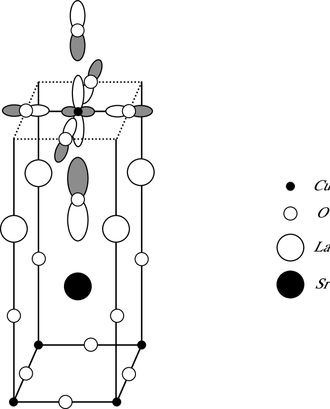
Figure 1: La₂CuO₄ with one doped Sr atom. Ab-initio calculationsub3lyp_dope find an A₁ hole localized above the Sr with hole character on the apical O $p_{z}$, Cu $z^{2}$, and planar O $p_{\sigma}$ orbitals. The $p_{z}$ character above the doped Cu is smaller than the $p_{z}$ below the Cu leading to an A₁ state rather than A_1g.

The polaron state with the hole delocalized over two diagonally opposed Cu in the four Cu plaquette is higher in energy in our ab-initio calculation by 0.57 eV for each Sr or 0.071 eV for each formula unit La_1.875Sr_0.125CuO₄. The value of 0.57 eV is an upper bound since our geometry optimizations only allowed the apical O sites to relax. The polaron localizes on two Cu sites due to spin exchange coupling with the $x^{2}-y^{2}$ hole and the anti-ferromagnetic spin ordering of the $x^{2}-y^{2}$ holes in our periodic supercells. In this paper, the hole state in figure 1 obtained from our ab-initio calculations is not taken to be the correct polaron. Instead, we postulate Sr doping leads to chiral polarons over the four plaquette Cu atoms shown in figure 2. This is discussed in section III.

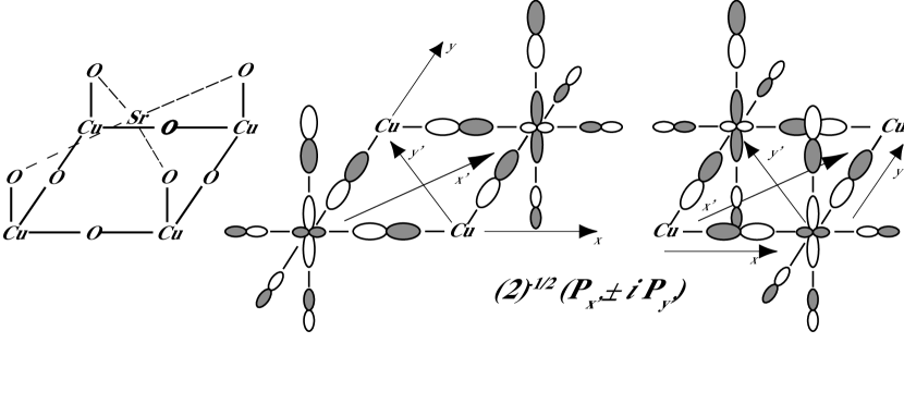
Figure 2: Orbital schematic of chiral polarons postulated in our model. We assume these chiral hole states are the most stable due to interactions with the undoped $d^{9}$ Cu lattice spins.

This paper explores the consequences of the assumptions that Sr doping causes holes to appear in Cu four-site plaquettes and the most stable configurations are the chiral states $P_{x^{\prime}}\pm iP_{y^{\prime}}$.

From an ab-initio standpoint, our first assumption is plausible for La_2-xSr_xCuO₄, but unproven. This may be due to the limitation of the special periodic supercells that were chosen out of necessity to perform the computation, the restrictive geometry relaxation for the plaquette polaron, or it may be a limitation of the B3LYP functional.

For YBa₂Cu₃O_6+δ, we do not have ab-initio proof for doping of four-site Cu plaquettes in the CuO₂ plane either. In fact, any polaron plaquettes would likely be in the yz plane where the Cu$-$O chains are along the y-axis and the z-axis is normal to the CuO₂ planes. One way in which polaron plaquettes can arise is when two adjacent Cu$-$O chains each have an occupied O separated by one lattice spacing along the x-axis (perpendicular to the direction of the chains). In other words, the two chain O reside in neighboring chains with minimum separation between them. This may create four-site polarons on the two CuO₂ planes above and below the two O atoms. For this paper, the chiral plaquette polarons in figure 2 are assumed.

The second assumption, that the polarons are chiral, is true for a localized polaron interacting with an infinite $d^{9}$ antiferromagnetic lattice in two dimensions (2D)siggia1 ; siggia2 ; siggia3 ; zee1 ; gooding1 by mapping the 2D Heisenberg antiferromagnet to a continuum model and analyzing the effective Hamiltonian arising from a path integral formulation. These papers did not specifically consider an out-of-plane hole, but the analysis is applicable in our scenario. This is discussed further in section III.

II.2 Experiment

Resonance circular dichroism photoemission investigating the spin of the occupied states near the Fermi level brookes1 ; brookes2 find a preponderance of singlet occupied states just below the Fermi level in CuO and Bi₂Sr₂CaCu₂O_8+δ (2212). These results are considered strong evidence in favor of the correctness of the t-J model. In particular, it is expected that out-of-plane $p_{z}$, $z^{2}$, and A_1g $p_{\sigma}$ would lead to triplet occupied states near E_F due to exchange Coulomb coupling to the orthogonal $x^{2}-y^{2}$ orbital. Since the prima facie evidence is against our proposal, we review the measurement and its interpretation.

We show our assumption of a delocalized $x^{2}-y^{2}$ band on the percolating out-of-plane polaron doped Cu sites leads to a null effect for resonance absorption on these sites. This arises because a delocalized $x^{2}-y^{2}$ band electron spin has no correlation to the polaron spin. Thus, the experiment measures the spin of the highest occupied states on the undoped Cu d⁹ sites where it is expected the first holes would be created in B_1g combinations of ligand planar O $p_{\sigma}$ orbitals that form a singlet with the $x^{2}-y^{2}$ d⁹ hole (the Zhang-Ricezhang_rice singlet).

The idea behind the dichroism experiment is to use circularly polarized incident soft x-rays tuned to the Cu L₃ ($2p_{3/2}$) white line energy ($\approx 931.5$ eV). The incident x-rays induce the photoabsorption transition $2p^{6}3d^{9}+\hbar\omega\rightarrow 2p^{5}d^{10}$ that Auger decays to an ARPES final state $2p^{6}d^{8}+e$. The spin-orbit energy separation of the core-hole $2p_{1/2}$ and $2p_{3/2}$ states is sufficiently large ($\sim 20$ eV) to guarantee the intermediate state is a $j=3/2$ core-hole.

By monitoring the outgoing electron energy and spin along the incident photon direction for each photon helicity, $\sigma^{+}$ and $\sigma^{-}$, the total spin of the final Cu d⁸ is obtained.

In the Bi-2212 experiment, brookes1 the photon is incident normal to the CuO₂ planes. The analysis below is for a normally incident photon. The transition rates are slightly different for the CuO casebrookes2 where a poly-crystalline sample was used.

Consider a Cu initially in the d⁹ state $|2p^{6};3d_{z^{2}}\uparrow\downarrow;3d_{x^{2}-y^{2}}(A_{\uparrow}\uparrow+A_{\downarrow}\downarrow)\rangle$, where our notation shows the occupied electrons. The $d_{xy}$, $d_{xz}$, $d_{yz}$ orbitals are always doubly occupied and are omitted in the wavefunction for convenience. The $3d_{z^{2}}$ orbital is doubly occupied and the single $x^{2}-y^{2}$ electron is in a spin state along a direction that may be different from the incident photon direction. It is represented as a linear combination of $\uparrow$ and $\downarrow$ along the incident photon direction with $|A_{\uparrow}|^{2}+|A_{\downarrow}|^{2}=1$. By summing over all helicities and exiting electron spin directions, the photoemission becomes independent of the initial direction of the $x^{2}-y^{2}$ electron as shown below.

Writing $\hat{x}$, $\hat{y}$, and $\hat{z}$ for the angular part of the Cartesian variables, $x/r$, $y/r$, and $z/r$, the relevant wave functions and photon polarization operators may be written as $d_{3z^{2}-r^{2}}=C_{2}(3\hat{z}^{2}-1)$, $d_{x^{2}-y^{2}}=\sqrt{3}C_{2}(\hat{x}^{2}-\hat{y}^{2})$, and $Y_{1\pm 1}=C_{1}(1/\sqrt{2})(\hat{x}\pm\hat{y})$, where $C_{1}=\sqrt{3/4\pi}$ and $C_{2}=\sqrt{5/16\pi}$. The mod-squared matrix elements for resonance absorption of $|2p^{6};3d_{z^{2}}\uparrow\downarrow;3d_{x^{2}-y^{2}}(A_{\uparrow}\uparrow+A_{\downarrow}\downarrow)\rangle$ to the intermediate $2p_{3/2}$ core-hole states are,

$$|2p^{6};3d_{z^{2}}\uparrow\downarrow;3d_{x^{2}-y^{2}}(A_{\uparrow}\uparrow+A_{\downarrow}\downarrow)\rangle$$

$$\stackrel{{\scriptstyle\hbar\omega^{+}}}{{\longrightarrow}}\left\{\begin{array}[]{llr}\left|p^{5}:\frac{3}{2},\frac{3}{2}\right\rangle d^{10}&=&|A_{\uparrow}|^{2}\\ \left|p^{5}:\frac{3}{2},\frac{1}{2}\right\rangle d^{10}&=&\frac{1}{3}|A_{\downarrow}|^{2}\end{array}\right\}\cdot\frac{1}{6}\left(\frac{C_{1}}{C_{2}}\right),$$ (3)

$$|2p^{6};3d_{z^{2}}\uparrow\downarrow;3d_{x^{2}-y^{2}}(A_{\uparrow}\uparrow+A_{\downarrow}\downarrow)\rangle$$

$$\stackrel{{\scriptstyle\hbar\omega^{-}}}{{\longrightarrow}}\left\{\begin{array}[]{llr}\left|p^{5}:\frac{3}{2},-\frac{3}{2}\right\rangle d^{10}&=&|A_{\downarrow}|^{2}\\ \left|p^{5}:\frac{3}{2},-\frac{1}{2}\right\rangle d^{10}&=&\frac{1}{3}|A_{\uparrow}|^{2}\end{array}\right\}\cdot\frac{1}{6}\left(\frac{C_{1}}{C_{2}}\right),$$ (6)

where $\hbar\omega^{\pm}$ are positively and negatively circularly polarized photons.

The Auger scattering rates of the four $2p_{3/2}$ intermediate states where one $x^{2}-y^{2}$ electron fills the $2p_{3/2}$ core hole and the other is ejected are,

$$\left|\frac{3}{2},\frac{3}{2}\right\rangle d^{10}\longrightarrow|2p^{6}\rangle|d_{z^{2}}\uparrow\downarrow\rangle+e\uparrow=|V|^{2},$$ (7)

$$\left|\frac{3}{2},\frac{1}{2}\right\rangle d^{10}\longrightarrow\left\{\begin{array}[]{c}|2p^{6}\rangle|d_{z^{2}}\uparrow\downarrow\rangle+e\uparrow=\left(\frac{2}{3}\right)|V|^{2},\\ |2p^{6}\rangle|d_{z^{2}}\uparrow\downarrow\rangle+e\downarrow=\left(\frac{1}{3}\right)|V|^{2},\end{array}\right.$$ (8)

$$\left|\frac{3}{2},-\frac{1}{2}\right\rangle d^{10}\longrightarrow\left\{\begin{array}[]{c}|2p^{6}\rangle|d_{z^{2}}\uparrow\downarrow\rangle+e\uparrow=\left(\frac{1}{3}\right)|V|^{2},\\ |2p^{6}\rangle|d_{z^{2}}\uparrow\downarrow\rangle+e\downarrow=\left(\frac{2}{3}\right)|V|^{2},\end{array}\right.$$ (9)

$$\left|\frac{3}{2},-\frac{3}{2}\right\rangle d^{10}\longrightarrow|2p^{6}\rangle|d_{z^{2}}\uparrow\downarrow\rangle+e\downarrow=|V|^{2},$$ (10)

where $|V|^{2}$ is the Auger matrix element. The $z^{2}$ is doubly occupied making the $d^{8}$ state a singlet. There are analogous matrix elements if the Auger process scatters the two $z^{2}$ electrons instead of $x^{2}-y^{2}$and also if the final $d^{8}$ is composed of one electron in $z^{2}$ and one in $x^{2}-y^{2}$ in a singlet configuration.

The total scattering rate is given by the products through the various intermediate states. Using the convention brookes1 ; brookes2 $\sigma^{+}\uparrow$, $\sigma^{-}\uparrow$, $\sigma^{+}\downarrow$, and $\sigma^{-}\downarrow$ to represent a positively circularly polarized photon ejecting an electron with $\uparrow$ spin etc, the scattering leaving a singlet $d^{8}$ final state is,

$$\sigma^{+}\uparrow = \left(|A_{\uparrow}|^{2}+\frac{2}{9}|A_{\downarrow}|^{2}\right)|V|^{2},$$ (11)

$$\sigma^{+}\downarrow = \frac{1}{9}|A_{\downarrow}|^{2}|V|^{2},$$ (12)

$$\sigma^{-}\uparrow = \frac{1}{9}|A_{\uparrow}|^{2}|V|^{2},$$ (13)

$$\sigma^{-}\downarrow = \left(\frac{2}{9}|A_{\uparrow}|^{2}+|A_{\downarrow}|^{2}\right)|V|^{2}.$$ (14)

The total parallel and anti-parallel scattering is,

$$\uparrow\uparrow\equiv(\sigma^{+}\uparrow+\sigma^{-}\downarrow) = \frac{11}{9}|V|^{2},$$ (15)

$$\uparrow\downarrow\equiv(\sigma^{+}\downarrow+\sigma^{-}\uparrow) = \frac{1}{9}|V|^{2},$$ (16)

where we have neglected the $(C_{1}/6C_{2})$ from equations II.2 and II.2 since it cancels out when we evaluate the polarization defined below. These two sums are independent of the starting spin orientation of the $x^{2}-y^{2}$ electron. The “polarization,” defined as a ratio $(\uparrow\uparrow-\uparrow\downarrow)/(\uparrow\uparrow+\uparrow\downarrow)=5/6$ for pure singlet $d^{8}$ states.

There are three possible triplet $d^{8}$ spin states. There is one electron in $x^{2}-y^{2}$ and $z^{2}$. The scattering from the intermediate $d^{10}$ state with a $2p_{3/2}$ core-hole to triplet $d^{8}$ is given by,

$$\left|\frac{3}{2},\frac{3}{2}\right\rangle d^{10}\rightarrow\left\{\begin{array}[]{l}|2p^{6}\rangle|\downarrow\downarrow\rangle+e\downarrow=2|V|^{2},\\ |2p^{6}\rangle|\frac{\uparrow\downarrow+\downarrow\uparrow}{\sqrt{2}}\rangle+e\uparrow=|V|^{2},\end{array}\right.$$ (17)

$$\left|\frac{3}{2},\frac{1}{2}\right\rangle d^{10}\rightarrow\left\{\begin{array}[]{l}|2p^{6}\rangle|\downarrow\downarrow\rangle+e\downarrow=\left(\frac{2}{3}\right)\cdot 2|V|^{2},\\ |2p^{6}\rangle|\frac{\uparrow\downarrow+\downarrow\uparrow}{\sqrt{2}}\rangle+e\uparrow=\left(\frac{2}{3}\right)|V|^{2},\\ |2p^{6}\rangle|\frac{\uparrow\downarrow+\downarrow\uparrow}{\sqrt{2}}\rangle+e\downarrow=\left(\frac{1}{3}\right)|V|^{2},\\ |2p^{6}\rangle|\uparrow\uparrow\rangle+e\uparrow=\left(\frac{1}{3}\right)\cdot 2|V|^{2},\end{array}\right.$$ (18)

$$\left|\frac{3}{2},-\frac{1}{2}\right\rangle d^{10}\rightarrow\left\{\begin{array}[]{l}|2p^{6}\rangle|\downarrow\downarrow\rangle+e\downarrow=\left(\frac{1}{3}\right)\cdot 2|V|^{2},\\ |2p^{6}\rangle|\frac{\uparrow\downarrow+\downarrow\uparrow}{\sqrt{2}}\rangle+e\downarrow=\left(\frac{2}{3}\right)|V|^{2},\\ |2p^{6}\rangle|\frac{\uparrow\downarrow+\downarrow\uparrow}{\sqrt{2}}\rangle+e\uparrow=\left(\frac{1}{3}\right)|V|^{2},\\ |2p^{6}\rangle|\uparrow\uparrow\rangle+e\uparrow=\left(\frac{2}{3}\right)\cdot 2|V|^{2},\end{array}\right.$$ (19)

$$\left|\frac{3}{2},-\frac{3}{2}\right\rangle d^{10}\rightarrow\left\{\begin{array}[]{l}|2p^{6}\rangle|\uparrow\uparrow\rangle+e\uparrow=2|V|^{2},\\ |2p^{6}\rangle|\frac{\uparrow\downarrow+\downarrow\uparrow}{\sqrt{2}}\rangle+e\downarrow=|V|^{2}.\end{array}\right.$$ (20)

Multiplying by the transition rates to the intermediate state for all possible photon and electron spin polarizations,

$$\sigma^{+}\uparrow = (|A_{\uparrow}|^{2}+\frac{4}{9}|A_{\downarrow}|^{2})|V|^{2},$$ (21)

$$\sigma^{+}\downarrow = (2|A_{\uparrow}|^{2}+\frac{5}{9}|A_{\downarrow}|^{2})|V|^{2},$$ (22)

$$\sigma^{-}\uparrow = (\frac{5}{9}|A_{\uparrow}|^{2}+2|A_{\downarrow}|^{2})|V|^{2},$$ (23)

$$\sigma^{-}\downarrow = (\frac{4}{9}|A_{\uparrow}|^{2}+|A_{\downarrow}|^{2})|V|^{2}.$$ (24)

The total parallel and anti-parallel scattering is,

$$\uparrow\uparrow\equiv(\sigma^{+}\uparrow+\sigma^{-}\downarrow) = \frac{13}{9}|V|^{2},$$ (25)

$$\uparrow\downarrow\equiv(\sigma^{+}\downarrow+\sigma^{-}\uparrow) = \frac{23}{9}|V|^{2},$$ (26)

leading to polarization $(\uparrow\uparrow-\uparrow\downarrow)/(\uparrow\uparrow+\uparrow\downarrow)=-(1/3)(5/6)$ for pure triplet $d^{8}$ states.

The measured value of the polarization for each photoelectron energy gives an estimate of the amount of singlet and triplet character in the occupied states below E_F. The experimentsbrookes1 ; brookes2 find singlet character just below E_F consistent with the t-J model and in contradiction to A₁ holes that would Hund’s rule triplet couple to the $x^{2}-y^{2}$ electron.

In our model, there are two types of Cu sites. The first is undoped with a single $x^{2}-y^{2}$ hole in a $d^{9}$ state. The ejected photoelectron near the Fermi level comes from the B_1g combination of neighboring $p_{\sigma}$ orbitals on the planar O that couples to the $x^{2}-y^{2}$ electron in a singlet as described by Zhang and Rice.zhang_rice This is consistent with experiment and the t-J model.

The second Cu is on a doped site with an out-of-plane polaron and a delocalized band comprised of $x^{2}-y^{2}$ and $p_{\sigma}$ in our model. In this case, the final Cu $d^{8}$ state has one $z^{2}$ and one $x^{2}-y^{2}$ hole with no spin correlation between them. Thus, $\uparrow\uparrow=\uparrow\downarrow$ and the “polarization” arising from resonance scattering on doped Cu sites is zero. The only polarization observed arises from the undoped sites with singlet holes near the Fermi energy.

The second experiment we consider is polarized xray absorption on La_2-xSr_xCuO₄ for $x=0.04-0.30$.xray1 ; pellegrin1 A substantial O absorption with z-axis polarized xrays indicates there are holes in apical O $p_{z}$. In addition, xray absorption fine structure (XAFS) haskel_Sr1 ; haskel_Sr2 measurements observe displacement of the apical O away from the Sr towards Cu consistent with hole formation in O $p_{z}$. Since the $p_{z}$ hole character is compatible with our out-of-plane polaron assumption, we focus on the Cu result.

The Cu absorption finds a few percent $z^{2}$ character on the Cu sites. Our ab-initio calculations find the $z^{2}$ hole character to be approximately 85% of the $x^{2}-y^{2}$ hole character. It is too large compared with experiment. One could argue that the many-body response to the formation of a Cu $2p$ core-hole is different for an undoped Cu versus a doped Cu where the delocalized $x^{2}-y^{2}$ band may suppress the white line due to the orthogonality catastrophe or more strongly screen the core-hole potential. We are not convinced this is the sole reason for the small amount of $z^{2}$ hole character observed in the white line.

A possible explanation is that the chiral polaron, spread out over four Cu sites as in figure 2, has more $p_{\sigma}$ and $p_{z}$ character at the expense of $z^{2}$ from delocalization compared to the polaron centered around a single Cu site in figure 1. A recent neutron pair distribution analysisbillinge is more compatible with a chiral plaquette polaron. In this case, extracting a very small signal from a bulk average of bond distances and then using the measured bond distances to infer orbital occupations is very model dependent.

III Chiral Polarons

The higher energy anti-bonding electronic states with apical $p_{z}$, $z^{2}$, and $p_{\sigma}$ over a four Cu doped plaquette are shown in figure 3. The $P_{x^{\prime}}$ and $P_{y^{\prime}}$ are degenerate. For simplicity, we have taken the two apical O $p_{z}$ above and below each Cu and the Cu $z^{2}$ and 4s to be one A₁ orbital. Thus, there are a total of eight states. The figure does not show the lower energy three bonding states (E and B₂) since they are occupied.

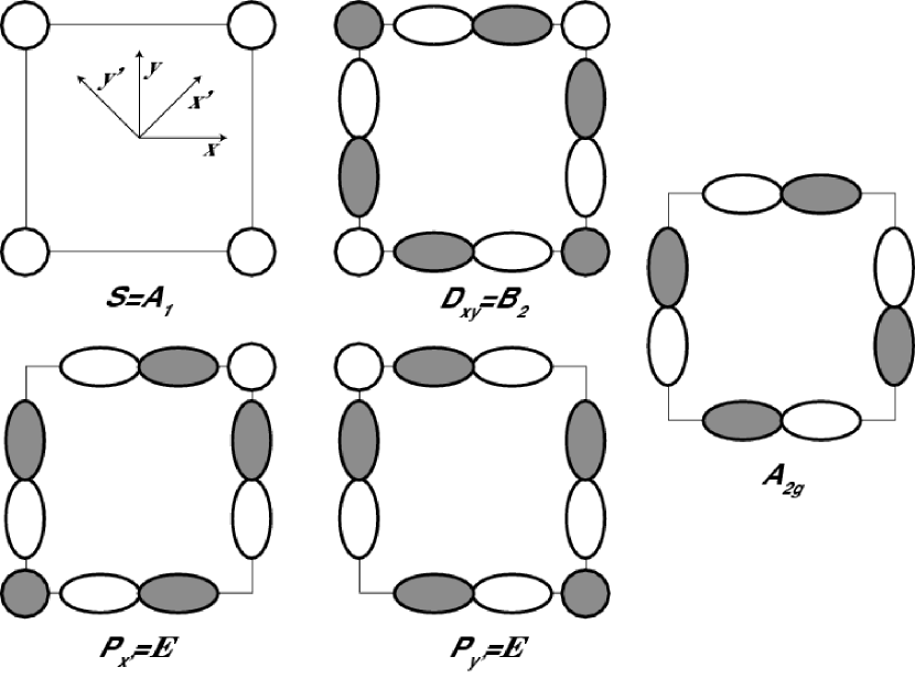
Figure 3: Projection onto CuO₂ of four polaron states and their symmetries. The higher energy anti-bonding states are shown. The fifth state of A_2g symmetry is composed entirely of $p_{\sigma}$ orbitals and is not a polaron state. This state becomes part of the delocalized $x^{2}-y^{2}$ band at the unoccupied $k$ state $(\pi,\pi)$ and the occupied bonding $x^{2}-y^{2}$, $p_{\sigma}$ band. We assume interaction with the undoped $d^{9}$ spin background, as shown in prior work, siggia1 ; siggia2 ; siggia3 ; zee1 ; gooding1 makes the chiral combinations $P_{x^{\prime}}\pm iP_{y^{\prime}}$ the most unstable electronic states (most stable hole states). When these chiral states percolate through the crystal, we further assume the electronic states composed of $x^{2}-y^{2}$ and $p_{\sigma}$ delocalize over these doped sites. There are a total of eight states. The lowest three have E (P${}_{x^{\prime}}$ and P${}_{y^{\prime}}$) and B₂ (D_xy) symmetry and are bonding combinations of the states in the figure. They are always occupied. The energies of the states are listed in table 2

Table 2 lists the energies of the eight polaron states for the case where the orbital energy of the “effective” A₁ composed of $p_{z}$ and $z^{2}$, is taken to be equal to the $p_{\sigma}$ orbital energy, $\epsilon_{z}=\epsilon_{p}=0$. There is an effective hopping matrix element, $t_{pz}$, from $p_{z}$ to $p_{\sigma}$. $t_{pp}$ is the diagonal $p_{\sigma}$ matrix element. It is expected $0<t_{pz}<t_{pp}$.

Table 2: Polaron symmetries and energies from highest (most unstable electronic states) to lowest. The effective $p_{z}$ and $p_{\sigma}$ orbital energies are taken to be 0.

State	Symmetry	Energy
P${}_{x^{\prime}}$, P${}_{y^{\prime}}$	E	$+\sqrt{2}t_{pz}$
Dxy	B2	$-t_{pp}+\sqrt{t_{pp}^{2}+4t_{pz}^{2}}$
S	A1	0
P${}_{x^{\prime}}$, P${}_{y^{\prime}}$	E	$-\sqrt{2}t_{pz}$
Dxy	B2	$-t_{pp}-\sqrt{t_{pp}^{2}+4t_{pz}^{2}}$
Not Polaron	A2	Coupled to $x^{2}-y^{2}$

Antiferromagnetic (AF) interaction of the polaron spin with the undoped Cu $d^{9}$ lattice renormalizes these couplings, but we expect P${}_{x^{\prime}}$ and P${}_{y^{\prime}}$ to remain the most unstable electronic states.

The effect of the undoped $d^{9}$ spin background is seen in mean-field where the $d^{9}$ AF spins surrounding a plaquette are frozen with an $\uparrow$ spin on one sublattice and a $\downarrow$ spin on the other sublattice. The additional energy of an $S$ or $D_{xy}$ polaron with spin $\sigma$ due to AF coupling of $\sigma$ with the $d^{9}$ spins is zero since the average $d^{9}$ spin seen by the polaron is zero. For $P$ states, the polaron spin couples to one sublattice. $\sigma$ can be aligned with the sublattice spin leading to a further destabilization of the $P$ state.

$P$ hole states were found in the exact diagonalization of Goodinggooding1 for a t-J model on a $4\times 4$ lattice with an additional hole allowed to delocalize on the interior $2\times 2$ lattice. This is in accordance with theoretical predictions. siggia1 ; siggia2 ; siggia3 ; zee1

Based on the energies in table 2, the mean-field description of the $d^{9}$ spins, and exact results on a $4\times 4$ lattice,gooding1 we assume the polaron hole has $P$ symmetry.

For a single hole delocalized in a small region of an AF spin background, it has been shownsiggia1 ; siggia2 ; siggia3 ; zee1 the chiral states $1/\sqrt{2}(P_{x^{\prime}}\pm iP_{y^{\prime}})$ are the correct spontaneous symmetry breaking states for the hole rather than P${}_{x^{\prime}}$ and P${}_{y^{\prime}}$, because the complex linear combinations are compatible with the long range twisting of the AF lattice spins into a stable configuration topologically distinct from the AF ground state.polyakov

In this paper, we assume doping introduces hole character in out-of-plane orbitals that can delocalize over a small number of sites in the vicinity of the dopant. The most favorable configuration for the polaron is taken to be the chiral state. If there was a single dopant in an infinite $d^{9}$ crystal, then the chiral states, $1/\sqrt{2}(P_{x^{\prime}}\pm iP_{y^{\prime}})$, would be degenerate. These two states are time-reversed partners.

In a finitely doped system, the environment of each polaron is different and the two chiral states may have different energies. We assume, in a doped cuprate, the chiral states are the correct polaron eigenstates, but the energies of the two states may be different. This leads to a model of the polarons where the splitting between the chiral states along with all the other states represented in table 2 and figure 3 are distributed differently for each plaquette. The assumption of a completely uniform probability distribution of different polaron state energies throughout the crystal leads to neutron $\omega/T$ scaling as shown in section V.1. A linear resistivity, derived in section VII, arising from the Coulomb scattering of $x^{2}-y^{2}$ band electrons with the polarons is also obtained with a uniform energy distribution.

This model of non-degenerate chiral polarons implies time-reversal symmetry is broken. At any instant, the number of “up” chiral polarons should equal the number of “down” chiral polarons and macroscopically the cuprate is time-reversal invariant. There is recent experimental evidence for local time-reversal symmetry breaking in neutron scattering. neutron_TR

IV Percolation

There are three basic assumptions of our model. First, doping leads to additional holes in out-of-plane orbitals that form chiral states as shown in figures 2 and 3.

Second, when these polaron plaquettes percolate through the crystal, a band is formed with the $x^{2}-y^{2}$ and $p_{\sigma}$ orbitals on the percolating swath. This metallic band interacts with the $x^{2}-y^{2}$ hole $d^{9}$ spins on the undoped Cu sites and the plaquette polarons. The random distribution of impurities leads to a distribution of the energy separations of polaron states shown in figure 3.

Third, this energy distribution is uniform. The linear resistivity arises from this assumption as shown in section VII. Since the resistivity is non-linear for certain dopings and temperature ranges, this assumption is not always valid.

The transition from spin-glass to superconductor in La_2-xSr_xCuO₄ at $x\approx 0.05$birgeneau_rmp and from an antiferromagnet to superconductor at $\delta\approx 0.35$ybco_af_sc in YBa₂Cu₃O_6+δ occur at the doping when the polarons percolate through the crystal.

In this section, the site percolation doping values are computed for La_2-xSr_xCuO₄ and YBa₂Cu₃O_6+δ. Reasonable assumptions for the distribution of plaquettes are used to approximately simulate the repulsion of the dopants. The computed values are close to known phase transitions in these materials.

We also computed the percolation for two additional systems. The first is La_2-xSr_xCuO₄ where each Sr dopes exactly one Cu site as shown in figure 1 and the second is a 2D square lattice with plaquette doping. The computed La_2-xSr_xCuO₄ 1-Cu percolation value of $x\approx 0.20$ is associated with the observed orthorhombic to tetragonal phase transition. birgeneau_rmp

For the 2D square lattice with four Cu plaquette doping, percolation occurs at $x\approx 0.15$. We believe the 2D percolation of the plaquettes should be associated with the transition from insulator to metal at $x\approx 0.15$ found by low temperature resistivity measurements in large pulsed magnetic fields.boeb1 This is further discussed in section VII.

All percolation computations described here were performed using the linear scaling algorithm of Newman and Ziff.ziff

In all these calculations, we simplify the problem by using Cu sites only. For La_2-xSr_xCuO₄, we take each Cu to have four neighbors in the plane at vectors $(\pm a,0,0)$, $(0,\pm b,0)$ and eight neighbors out of the plane at $(\pm a/2,\pm b/2,\pm c/2)$ where $a$, $b$, and $c$ are the cell dimensions. Thus, each Cu has a total of 12 neighbors in the site percolation calculations.

For all YBa₂Cu₃O_6+δ calculations, we take each planar Cu to be connected to a total of six Cu atoms. There are four nearest neighbors in the same CuO₂ plane, one neighboring Cu on the adjacent CuO₂ across the intervening Y atom and one Cu on the neighboring chain. The chain Cu is connected to the two Cu atoms in the CuO₂ planes above and below itself. We assume a chain O dopes three Cu atoms, two in CuO₂ planes and the corresponding chain Cu as shown in the constraints of figure 5.

Table 3 lists the computed percolation values for La_2-xSr_xCuO₄, a 2D square lattice, and YBa₂Cu₃O_6+δ for various types of doping and doping constraints. These constraints were chosen to simulate the repulsion of the dopants and are approximations to the actual distribution of dopants in the cuprates.

The La_2-xSr_xCuO₄ and YBa₂Cu₃O_6+δ calculations are on $200\times 200\times 200$ lattices with $2,500$ different dopings. The square lattice size is $2,000\times 2,000$ with $5,000$ different dopings.

Table 3: Percolation values for various structures and doping scenarios. The constraints column references the figures describing the applied constraint. All La_2-xSr_xCuO₄ and YBa₂Cu₃O_6+δ results are obtained for a $200\times 200\times 200$ lattice with $2,500$ doped ensembles. The percolation value is the computed critical $x$ in La_2-xSr_xCuO₄ and $\delta$ in YBa₂Cu₃O_6+δ. The square lattice results are for a $2,000\times 2,000$ lattice with $5,000$ ensembles. The digit in parentheses is the error in the last digit.

Structure	Dopant Type	Constraints	Percolation
LSCO	1-Cu	none	$0.19617(2)$
LSCO	4-Cu	none	$0.05164(1)$
LSCO	4-Cu	fig. 4a	$0.05097(1)$
LSCO	4-Cu	fig. 4a,b	$0.04834(1)$
LSCO	4-Cu	fig. 4a,b,c	$0.04880(1)$
LSCO	4-Cu	fig. 4a,b,c,e	$0.04904(1)$
LSCO	4-Cu	fig. 4a,b,e	$0.04862(1)$
LSCO	4-Cu	fig. 4a,b,c,d	$0.04926(1)$
LSCO	4-Cu	fig. 4a,b,c,d,e	$0.04943(1)$
Square	4-Cu	fig. 4a,b	$0.15053(1)$
YBCO	3-Cu	fig. 5a	$0.31162(2)$
YBCO	3-Cu	fig. 5b	$0.32890(2)$
YBCO	3-Cu	fig. 5b,c	$0.36098(2)$

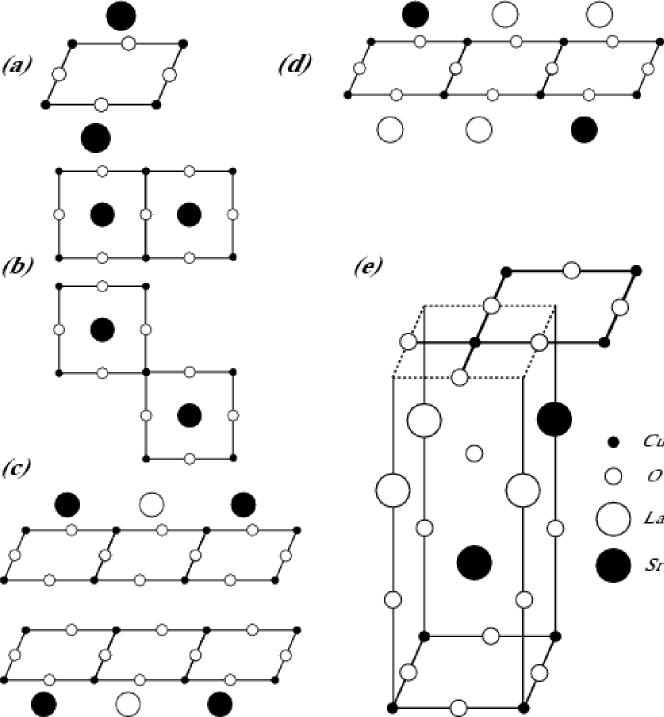
Figure 4: Applied Sr doping constraints used for the La_2-xSr_xCuO₄ and 2D square lattice plaquette percolation calculations shown in table 3. For each four Cu plaquette in figures 2 and 3, two Sr atoms, one above and one below the plaquette (upper and lower Sr), can dope the Cu’s. Each figure shows the disallowed configuration of Sr doping. It is assumed all $\pm 90^{\circ}$ and $180^{\circ}$ rotated configurations are equivalent to the figure and also disallowed. (a) an upper and lower Sr doping the same plaquette. (b) a Cu atom in a plaquette doped by two different Sr atoms. This figure includes the three cases of two upper Sr, two lower Sr, and one upper and one lower Sr. This is the no overlap constraint. (c) adjacent plaquettes doped by two upper Sr or two lower Sr. (d) adjacent plaquettes doped by one upper Sr and one lower Sr. (e) nearest neighbor upper Sr and lower Sr in different LaO planes.

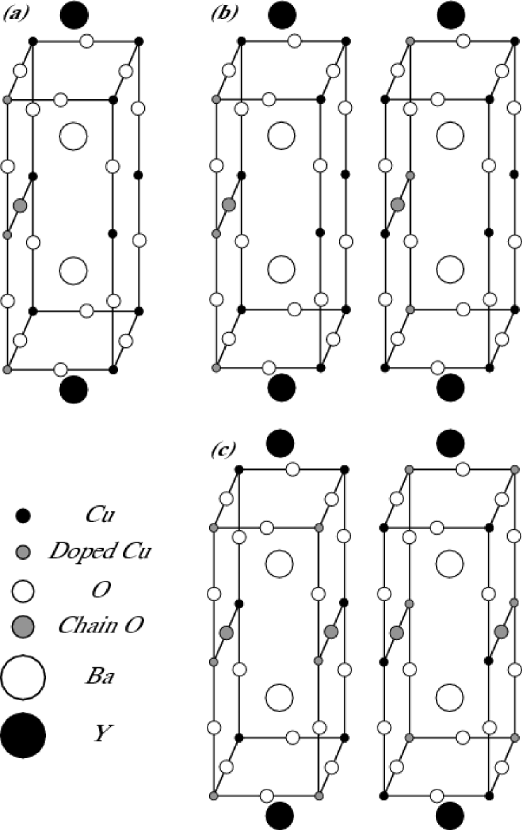
Figure 5: Doping constraints used for YBa₂Cu₃O_6+δ calculations shown in table 3. The chain O and its three doped Cu sites are shaded gray. Three different doping scenarios are shown. (a) the chain O dopes a fixed Cu triple. (b) the chain O randomly dopes one of the two possible Cu triples. No triple may be doped by two adjacent chain O. (c) If two chain O are in the same cell, the two Cu doping configurations where the triples are closest to each other are not permitted.

The first La_2-xSr_xCuO₄ calculation is the critical doping for percolation of doped Cu where each Sr dopes the single Cu shown in figure 1 instead of the four Cu plaquette of figure 2. Although we assume plaquettes are created at low dopings, once the doping is large enough, there is crowding of the plaquettes. Single Cu polarons are formed. This single Cu percolation calculation is an approximate measure of the doping for the transition from predominantly doped plaquettes to single site polarons. A phase transition at this crossover doping is expected. The computed percolation of $x\approx 0.20$ matches the orthorhombic to tetragonal transitionbirgeneau_rmp doping.

From the table, the critical doping for 3D plaquette percolation in La_2-xSr_xCuO₄ is $x\approx 0.05$ regardless of the applied doping constraints and matches the spin-glass to superconductor transition.birgeneau_rmp

This is because the plaquette percolation values are approximately $1/4$ of the single Cu percolation result of $x\approx 0.20$.

For YBa₂Cu₃O_6+δ, the more realistic doping constraints are the second and third cases where $\delta\approx 0.33$ and $\delta\approx 0.36$ since O chains should not have a preference for which Cu triple to dope. Experimentybco_af_sc finds $\delta\approx 0.35$.

From these results, we conclude the plaquette polaron model with percolation can obtain known insulator to metal phase transitions in La_2-xSr_xCuO₄ and YBa₂Cu₃O_6+δ.

V Neutron Scaling and Incommensurability

V.1 Scaling

Neutron spin scattering measures the imaginary part of the magnetic susceptibility, $\chi(\mathbf{q},\omega)$.

The integral of the imaginary part of the spin susceptibility $\int{\mathbf{d^{2}q}}\ \chi^{\prime\prime}({\mathbf{q}},\omega)$ over the Brillouin zone where $\chi=\chi^{\prime}+i\chi^{\prime\prime}$ has been found neutron_scaling1 ; neutron_scaling2 ; neutron_scaling3 ; neutron_scaling4 ; neutron_scaling5 ; neutron_scaling6 ; neutron_scaling7 to be a function of $\omega/T$. The integral is the on-site magnetic spin susceptibility.

The $\omega/T$ scaling is unusual because $\chi^{\prime\prime}\sim\omega/J_{dd}$ for an antiferromagnet and $\chi^{\prime\prime}\sim\omega/E_{F}$ for a band where $J_{dd}$ is the $d^{9}$ AF spin coupling and $E_{F}$ is the $x^{2}-y^{2}$ band Fermi energy.

In this section, we show that the single polaron susceptibility is a function of $\omega/T$ when the energy difference between polaron chiral states with opposite spins and chiralities is uniformly distributed.

The $\mathbf{q}$ dependence of the polaron susceptibility, $\chi_{p}^{\prime\prime}(\mathbf{q},\omega)$, is peaked at $\mathbf{q}=0$ if spin-flip polaron scattering dominates at low energy. $\chi_{p}^{\prime\prime}(\mathbf{q},\omega)$ is peaked at $\mathbf{q}=(\pi,\pi)$ if the polaron spin and chirality flip at low energy. The latter scatters the polaron to its time-reversed state. The time-reversed chiral polarons are the low energy excitations, as shown in section V.2. The $\mathbf{q}$ dependence is broad because the polaron is localized over a four-site plaquette. Since the total susceptibility is dominated by $\mathbf{q}$ near $(\pi,\pi)$, the polaron susceptibility is approximately momentum independent, $\chi_{p}^{\prime\prime}(\mathbf{q},\omega)\approx\chi_{p}^{\prime\prime}(\omega)$.

The imaginary part of the polaron susceptibility is found to be of the form $\chi_{p}^{\prime\prime}(\omega)\sim\tanh(\beta\omega/2)$ and satisfies scaling. The coupling of the polaron spin and chiral orbital state to the undoped $d^{9}$ spins causes the total susceptibility to become incommensurate. This is shown in the next subsection V.2 where we compute the static spin structure factor for classical spins perturbed by chiral polarons.

In this section, we show that coupling to the undoped $d^{9}$ spins leads to a dynamic susceptibility consistent with the measured form neutron_scaling1 ; birgeneau_rmp in equation 40.

Consider a polaron as in figure 6 with energy $\Delta$ separating the down spin state from the up spin and occupations $n_{\downarrow}$ and $n_{\uparrow}$ in thermal equilibrium. Since the polaron is always singly occupied, $n_{\uparrow}+n_{\downarrow}=1$ and $n_{\downarrow}=e^{\beta\Delta}n_{\uparrow}$. Solving for $n_{\downarrow}$ and $n_{\uparrow}$,

$$n_{\downarrow}=f(-\Delta),\ \ n_{\uparrow}=f(\Delta),$$ (27)

where $f(\epsilon)$ is the Fermi-Dirac function,

$$f(\epsilon)=\frac{1}{e^{\beta\epsilon}+1}.$$ (28)

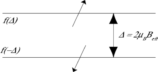
Figure 6: Energy difference $\Delta$ between an up and down spin polaron. $f(-\Delta)$ and $f(\Delta)$ are the equilibrium occupations of the spins states where $f(\epsilon)$ is the Fermi-Dirac function, $f(\epsilon)=1/(e^{\beta\epsilon}+1)$. B_eff is the effective magnetic field that splits the spin energies by $\Delta$. The chiralities of the two states are different for low energies leading to a broad peak in $\chi_{p}^{\prime\prime}(\mathbf{q},\omega)$ at $(\pi,\pi)$.

To compute the dynamical polaron spin susceptibility, consider an applied magnetic field $Be^{i\omega t}$ normal to the spin quantization axis. The alternating field induces transitions between the two states if $\Delta=\omega$.

Let $W=W_{\uparrow\downarrow}=W_{\downarrow\uparrow}$ be the induced transition rate between the two spin states. The total absorption rate is,

$$\left<P(\Delta)\right>=\hbar\omega W(n_{\downarrow}-n_{\uparrow}).$$ (29)

Using equation 27,

$$\left<P(\Delta)\right>=\hbar\omega W\left[f(-|\Delta|)-f(|\Delta|)\right],$$ (30)

$$\left<P(\Delta)\right>=\hbar\omega W\tanh(\beta|\Delta|/2).$$ (31)

The absolute values of $\Delta$ are used above because the absorption rate is independent of which spin state is lower in energy. The transition rate $W$ is,

$$W(\Delta)=\frac{2\pi}{\hbar}\mu_{B}^{2}B^{2}\delta(\omega-|\Delta|).$$ (32)

Averaging $W$ over all spin quantization directions multiplies equation 32 by $2/3$,

$$\langle W(\Delta)\rangle=\frac{4\pi}{3\hbar}\mu_{B}^{2}B^{2}\delta(\omega-|\Delta|).$$ (33)

Let $\rho(\Delta)$ to be the probability distribution of energy differences for spin and chirality flips. Summing over all polarons, the total absorption rate is,

$$\left<P(\omega)\right>=\hbar\omega\int d\Delta\ \rho(\Delta)\tanh(\beta|\Delta|/2)\langle W(\Delta)\rangle,$$ (34)

$$\left<P(\omega)\right>=\left(\frac{4\pi}{3}\right)\omega\mu_{B}^{2}B^{2}\left[\rho(\omega)+\rho(-\omega)\right]\tanh\left(\frac{\beta\omega}{2}\right),$$ (35)

$$\left<P(\omega)\right>=\left(\frac{8\pi}{3}\right)\omega\mu_{B}^{2}B^{2}\rho(\omega)\tanh\left(\frac{\beta\omega}{2}\right),$$ (36)

where $\rho(-\Delta)=\rho(\Delta)$ because there is an equal number of polarons with an up spin lower in energy than a down spin as there are down spins lower in energy than up spins.

The absorption rate can be written in terms of the imaginary part of the polaron susceptibility as,

$$\left<P(\omega)\right>=\frac{1}{2}\omega\chi_{p}^{\prime\prime}(\omega)B^{2},$$ (37)

leading to the imaginary susceptibility per polaron of,

$$\chi_{p}^{\prime\prime}(\omega)=\left(\frac{16\pi}{3}\right)\mu_{B}^{2}\rho(\omega)\tanh\left(\frac{\beta\omega}{2}\right).$$ (38)

The probability density of polaron energy separations $\rho(\Delta)$ is taken to be uniform with $\int d\Delta\rho(\Delta)=1$ and of the form,

$$\rho(\Delta)=\left\{\begin{array}[]{cc}\frac{1}{2\Delta_{\mathrm{max}}},&-\Delta_{\mathrm{max}}<\Delta<\Delta_{\mathrm{max}}\\ 0,&|\Delta|>\Delta_{\mathrm{max}}\end{array}\right.$$ (39)

where $\Delta_{\mathrm{max}}$ is doping dependent, $\Delta_{\mathrm{max}}=\Delta_{\mathrm{max}}(x)$.

Equations 38 and 39 show that the polaron susceptibility is a function of $\omega/T$ and has the approximate form seen in experiments.birgeneau_rmp ; neutron_scaling1 The functional form of $\chi_{p}^{\prime\prime}$ increasing from $\chi_{p}^{\prime\prime}(0)=0$ and saturating for $\beta\omega>1$ arises from the thermal occupations of polaron states with energy splitting $\omega$. When $\beta\omega\ll 1$, the two states have almost equal occupation and the absorbed energy is small from equations 29 and 30. For $\beta\omega\gg 1$, the lower energy state is always occupied and the higher energy spin state is always unoccupied. In this case, the absorption saturates. Since the polaron spin density $\rho(\Delta)$ is constant up to $\Delta_{\mathrm{max}}$, it is $\beta\omega$ that determines the amount of absorption due to the difference of the two Fermi-Dirac occupation factors. Finally, if there are no spin flip energies smaller than $\Delta_{\mathrm{min}}$, then $\chi_{p}^{\prime\prime}(\omega)$ is zero for $\omega<\Delta_{\mathrm{min}}$.

The measured susceptibility for La_2-xSr_xCuO₄ at $x=0.04$ is normalized and fit by the expression neutron_scaling1 ; birgeneau_rmp

$$\left(\frac{2}{\pi}\right)\tan^{-1}[a_{1}(\beta\omega)+a_{3}(\beta\omega)^{3}],$$ (40)

with $a_{1}=0.43$ and $a_{3}=10.5$. This curve rises to the saturating value of one faster than our expression in equation 38.

The contribution to the susceptibility from the undoped $d^{9}$ spins and the metallic $x^{2}-y^{2}$ band has not been included. The band contribution is on the order of $\omega/E_{f}$ where $E_{f}$ is the Fermi energy and can be neglected. The imaginary susceptibility from the undoped $d^{9}$ spins is on the orderpines_scaling1 of $\omega/\Gamma$ where $\Gamma$ is several $J_{dd}$ to $E_{f}$ and can also be neglected. The real part of the $d^{9}$ susceptibility is approximately constant up to the energy $\omega\sim\Gamma$. We may therefore take the $d^{9}$ susceptibility to be real and $\omega$ independent for small $\omega$. Thus, the $\omega$ dependence of the total susceptibility arises from the polaron susceptibility in equation 38.

The $\mathbf{q}$ dependence of the susceptibility is incommensurate from the calculations of the next section and of the form,pines_scaling1

$$\chi(\mathbf{q})=\frac{\mu_{B}^{2}\tilde{\chi}_{0}\left(\xi/a\right)^{2}}{1+\left(\mathbf{q}-\mathbf{Q}\right)^{2}\left(\xi/a\right)^{2}},$$ (41)

where $\mathbf{Q}$ is the incommensurability peak vector and $\xi$ is the correlation length. From the computations in the next section, $\mathbf{Q}$ is shifted from $(\pi/a,\pi/a)$ along the Cu$-$O bond direction and agrees with experiment. $\xi\approx a/\sqrt{x}$ is the mean separation between Sr.

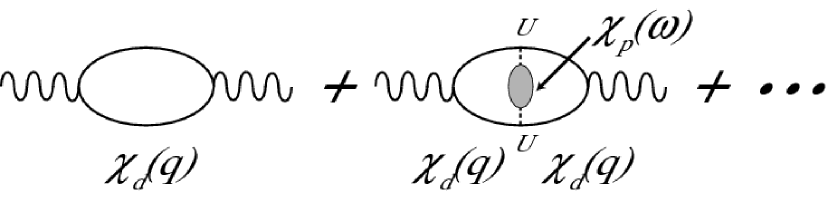
Figure 7: Diagrams to sum in the random phase approximation for the dynamic susceptibility $\chi(\mathbf{q},\omega)$. The first term is the static susceptibility $\chi(\mathbf{q})$ in equation 41 and the shaded loop is the polaron susceptibility $\chi_{p}(\omega)$ with imaginary part shown in equation 38. $U$ is the coupling energy.

Summing the random phase approximation diagrams in figure 7 leads to,

$$\left[\frac{\chi(\mathbf{q},\omega)}{\mu_{B}^{2}}\right]^{-1}=\left[\frac{\chi(\mathbf{q})}{\mu_{B}^{2}}\right]^{-1}-xU^{2}\left[\frac{\chi_{p}(\omega)}{\mu_{B}^{2}}\right],$$ (42)

$$\chi(\mathbf{q},\omega)=\frac{\mu_{B}^{2}\tilde{\chi}_{0}\left(\xi/a\right)^{2}}{1+\left(\mathbf{q}-\mathbf{Q}\right)^{2}\left(\xi/a\right)^{2}-\tilde{\chi}_{0}U^{2}\left[\chi_{p}(\omega)/\mu_{B}^{2}\right]},$$ (43)

where we have used $(\xi/a)^{2}x=1$ for the $\chi_{p}$ term.

Using the integral,

$$\mathrm{Im}\int\frac{d^{2}q}{A+Bq^{2}-iC}=\int_{0}^{+\infty}\frac{\left(2\pi C\right)qdq}{\left(A+Bq^{2}\right)^{2}+C^{2}},$$

$$=\left(\frac{\pi}{B}\right)\left[\frac{\pi}{2}-\tan^{-1}\left(\frac{A}{C}\right)\right]=\left(\frac{\pi}{B}\right)\tan^{-1}\left(\frac{C}{A}\right),$$ (44)

and defining $\tilde{\chi}_{p}(\omega)=\chi_{p}(\omega)/\mu_{B}^{2}$, the integrated imaginary susceptibility is,

$$\int\chi^{\prime\prime}(\mathbf{q},\omega)dq=\pi\mu_{B}^{2}\tilde{\chi}_{0}\tan^{-1}\left[\frac{\tilde{\chi}_{0}U^{2}\tilde{\chi}_{p}^{\prime\prime}(\omega)}{1-\tilde{\chi}_{0}U^{2}\tilde{\chi}_{p}^{\prime}(\omega)}\right].$$ (45)

In the above expression, $\tilde{\chi}_{p}=\tilde{\chi}_{p}^{\prime}+i\tilde{\chi}_{p}^{\prime\prime}$ has been expanded into real and imaginary parts.

Using $\chi_{p}^{\prime}(-\omega)=\chi_{p}^{\prime}(\omega)$ and $\chi_{p}^{\prime\prime}(-\omega)=-\chi_{p}^{\prime\prime}(\omega)$, the equation can fit the experimental curve in equation 40.

V.2 Incommensurability

There is an antiferromagnetic coupling, $J_{pd}$, between the polaron spin $\mathbf{S}_{p}$ and the neighboring $d^{9}$ spins. The polaron is delocalized over four Cu sites. The probability of the hole residing on a particular Cu is $1/4$ leading to the estimate $J_{pd}\approx(1/4)J_{dd}$ where $J_{dd}$ is the undoped $d^{9}$ AF coupling. The effective coupling of a chiral polaron to the $d^{9}$ spin background is known zee1 ; gooding1 ; gooding_birgeneau to induce a twist in the neighboring spins. This can be encapsulated in a topological charge termpolyakov of the form $\mp J_{ch}[{\mathbf{S}_{p}\cdot(\mathbf{S}_{1}\times\mathbf{S}_{2})}]$ where $\mathbf{S}_{p}$ is the polaron spin and $\mathbf{S}_{d1}$, $\mathbf{S}_{d2}$ are adjacent $d^{9}$ spins as shown in figure 8.

The expectation value $\langle{\mathbf{S}_{p}\cdot(\mathbf{S}_{1}\times\mathbf{S}_{2})}\rangle=0$ for states invariant under time reversal. Thus, the expectation value of the topological charge is zero for the real polaron states $P_{x^{\prime}}$, $P_{y^{\prime}}$, $S$, and $D_{xy}$. The complex linear combinations in the chiral states lead to non-zero topological charge. The above chiral coupling term is the simplest coupling of chiral polarons to the neighboring spins.

The referenceszee1 ; gooding1 ; gooding_birgeneau considered holes in both the t-J and three-band Hubbard models that can delocalize over a four-site plaquette. In our model, $x^{2}-y^{2}$ spins delocalize on the plaquettes forming a band when the polarons percolate. Our chiral coupling is between a polaron spin and the adjacent spin sites that may be undoped $d^{9}$ or another polaron spin. The specific form for the coupling is analogous to previous work.

The coupling of the $x^{2}-y^{2}$ band to the neighboring spins is smaller than the chiral coupling of the polaron and $d^{9}$ spins. The perturbation arising from the band spin coupling selects incommensurability along the Cu$-$O bond directions as shown at the end of this section.

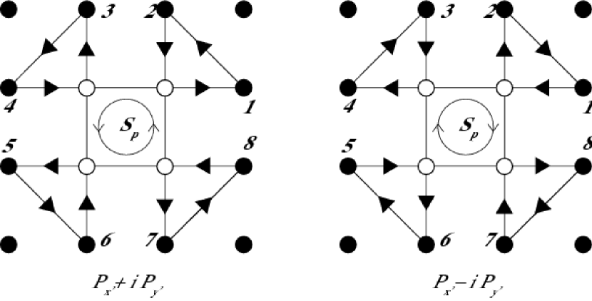
Figure 8: Coupling of chiral polarons to neighboring $d^{9}$ spins. $\mathbf{S}_{p}$ is the polaron spin and it couples to four $d^{9}$ pairs in the cyclic order shown by the arrows and equation 46. The chiral coupling for the $P_{x^{\prime}}-iP_{y^{\prime}}$ polaron reverses the cyclic ordering of the spins as seen in the figure and leads to the same expression as the $P_{x^{\prime}}+iP_{y^{\prime}}$ with $J_{ch}\rightarrow-J_{ch}$.

The polaron chiral coupling of $P_{x^{\prime}}\pm iP_{y^{\prime}}$ to the neighboring $d^{9}$ spins is,

$$\begin{array}[]{ccc}H_{ch}&=&\mp J_{ch}\left\{\mathbf{S_{p}}\cdot(\mathbf{S_{1}}\wedge\mathbf{S_{2}})+\mathbf{S_{p}}\cdot(\mathbf{S_{3}}\wedge\mathbf{S_{4}})+\right.\\ &&\left.\mathbf{S_{p}}\cdot(\mathbf{S_{5}}\wedge\mathbf{S_{6}})+\mathbf{S_{p}}\cdot(\mathbf{S_{7}}\wedge\mathbf{S_{8}})\right\},\end{array}$$ (46)

where $J_{ch}>0$ and the spins are labelled in figure 8. The antiferromagnetic coupling of polaron spins to undoped $d^{9}$ spins is

$$H_{pd}=J_{pd}\mathbf{S_{p}}\cdot\left(\mathbf{S_{1}}+\dots+\mathbf{S_{8}}\right).$$ (47)

Electronic hopping matrix elements are on the order of $0.5-1.0$ eV. The chiral coupling, $J_{ch}$, is estimated to be less than or of the same order. Gooding et al.gooding_mailhot1 obtain $J_{ch}\approx 3J_{dd}$ from numerical simulations and by computing the effective next-nearest neighbor antiferromagnetic coupling, $J^{\prime}_{dd}$, induced by chiral polarons at very low doping. $J^{\prime}_{dd}$ is then compared with Raman data to obtain $J_{ch}$.

In the spin Hamiltonian of Gooding et al.,gooding_mailhot1 the chiral coupling term is squared, $-J_{ch}[\mathbf{S_{1}}\cdot(\mathbf{S_{2}}\wedge\mathbf{S_{3}})]^{2}$, in contrast to our linear terms in equation 46. The overall energy scale of $J_{ch}$ is similar. We take $J_{ch}=3J_{dd}$ where $J_{dd}\approx 0.1$ eV in our computations of the static neutron structure factor. We have found our results for the magnitude of the incommensurability are independent of the precise values of all of the parameters. The only necessary feature to obtain incommensurability is that the chiral coupling, $J_{ch}$, is sufficiently large to break the $(\pi,\pi)$ spin ordering from the antiferromagnetic spin coupling, $J_{dd}$.

There is an antiferromagnetic spin-spin coupling between the polarons. $J_{pp}$ is the coupling between $\mathbf{S_{p1}}$ and $\mathbf{S_{p2}}$ and $J^{\prime}_{pp}$ is the coupling between $\mathbf{S_{p1}}$ and $\mathbf{S_{p3}}$ shown in figure 9. An estimate of $J_{pp}$ and $J^{\prime}_{pp}$ is obtained in a similar manner to $J_{pd}$. For $J_{pp}$, the polarons have two adjacent pair sites. An antiferromagnetic coupling occurs for every adjacent pair. This occurs with probability $(1/4)^{2}=1/16$. There are two pairs for $J_{pp}$ and one for $J^{\prime}_{pp}$ leading to estimates $J_{pp}\approx(1/8)J_{dd}$ and $J^{\prime}_{pp}\approx(1/16)J_{dd}$.

Figure 9 shows various chiral couplings when polarons are adjacent to each other. Using a similar analysis, we estimate the magnitude of the chiral couplings to be, $J_{ppp}\approx(1/4)^{2}J_{ch}$, $J_{ppd}\approx(1/4)J_{ch}$, and $J^{\prime}_{ppd}\approx(1/4)J_{ch}$.

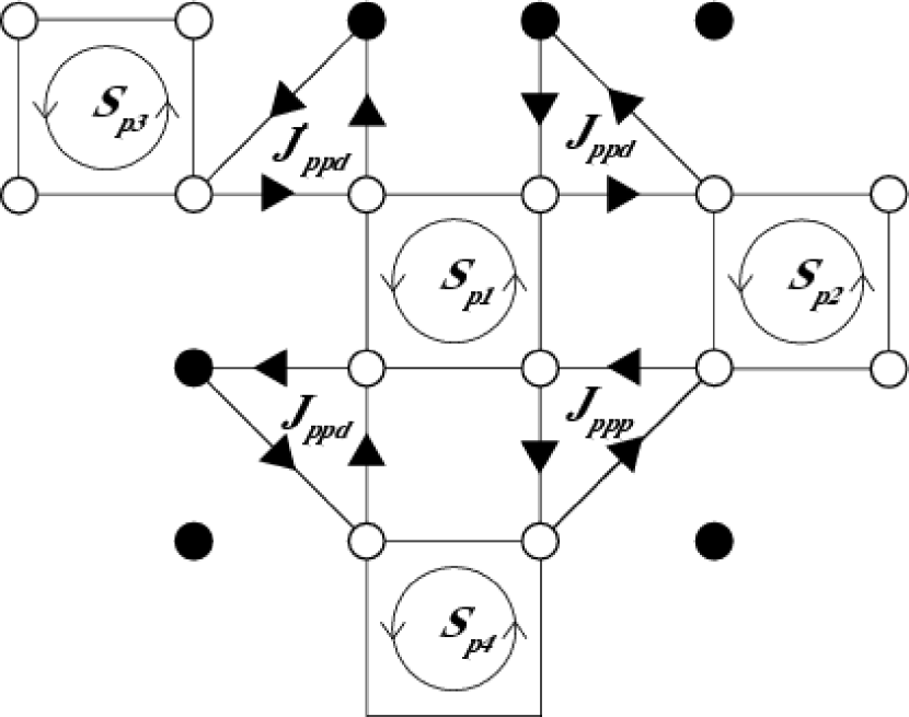
Figure 9: Schematic of adjacent polaron configurations. $J_{ppp}$ is the chiral coupling between three polarons, $J_{ppd}$ couples two polarons to a $d^{9}$ spin, and $J^{\prime}_{ppd}$ couples two polarons to a $d^{9}$ spin when one polaron is shifted by one lattice spacing. The couplings are shown for the case where all the polarons are $P_{x^{\prime}}+iP_{y^{\prime}}$. For each opposite chirality polaron, $P_{x^{\prime}}-iP_{y^{\prime}}$, the coupling should be multiplied by $-1$. The figure does not exhaust all possible couplings. For example, there is another term $J^{\prime}_{ppp}$ if $\mathbf{S_{p4}}$ is shifted to the right by one lattice spacing.

The total spin Hamiltonian for the $d^{9}$ spins and polarons is

$$H=H_{dd}+H_{pd}+H_{pp}+H_{ch}^{tot},$$ (48)

where $H_{dd}$ is the antiferromagnetic $d^{9}$ spin-spin coupling with $J_{dd}\approx 0.1$ eV. $H_{pd}$ is the polaron-$d^{9}$ coupling and $H_{pp}$ is the polaron-polaron spin coupling. $H_{ch}^{tot}$ is the total chiral coupling.

The chiral coupling $H_{ch}^{tot}$ is invariant under polaron time reversal that flips the chirality of a single polaron $P_{x^{\prime}}\pm iP_{y^{\prime}}\rightarrow P_{x^{\prime}}\mp iP_{y^{\prime}}$ or $(J_{ch}\rightarrow-J_{ch})$ and the polaron spin, $\mathbf{S_{p}}\rightarrow\mathbf{-S_{p}}$. $H_{pd}\rightarrow-H_{pd}$ is not invariant under time reversal of the polaron. When the chiral coupling is much larger than all spin-spin couplings, $J_{ch}\gg J_{dd}>J_{pd}>J_{pp}>J^{\prime}_{pp}$, the ground state energy becomes independent of the polaron chiralities.

This is an important point because it means the energy to simultaneously flip the chirality and spin of a polaron has an energy scale $J_{dd}$ while flipping either the chirality or the spin, but not both, has an energy scale $J_{ch}$.

Figure 10 shows the minimized spin ordering surrounding a polaron when the chiral coupling, $J_{ch}$, dominates the polaron spin to $d^{9}$ coupling, $J_{pd}$. Increasing $J_{ch}$ further does not change the spin ordering. This leads to an incommensurability that is weakly parameter dependent. All the neighboring $d^{9}$ spins in the figure are orthogonal to the polaron spin. The $H_{pd}$ antiferromagnetic energy is zero. The energy difference of the time reversed polaron in the same background is also zero. The spin-spin couplings, $J_{pd}$ etc, lead to non-zero energy differences.

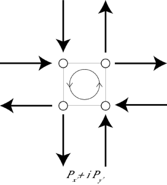
Figure 10: Minimized energy configuration for a polaron with spin pointing out of the page surrounded by 8 $d^{9}$ spins. Only $J_{dd}$ and $J_{ch}$ are non-zero. This represents the regime dominated by $J_{ch}$.

The static neutron spin structure factor is computed by minimizing the energy in equation 48 on a finite 2D lattice with classical spins $\mathbf{S}_{i}$ of unit length, $\mathbf{S}_{i}^{2}=1$. Each undoped $d^{9}$ site has a spin and every polaron has an orbital chirality, $P_{x^{\prime}}\pm iP_{y^{\prime}}$, and spin. All the terms for the classical Hamiltonian are described above along with the parameters used. The only constraint on the polarons is that they may not overlap, but otherwise they are randomly placed in the lattice. At this point, the effect of the delocalized $x^{2}-y^{2}$ band electrons is ignored.

One can imagine additional constraints on the placement of the polarons arising from polaron-polaron Coulomb repulsion. Also, calculations on 3D lattices with a small interlayer antiferromagnetic spin coupling can be done. The addition of polaron constraints and the third dimension does not to change the computed incommensurability or its location in the Brillouin zone. These effects are ignored in this paper.

Finally, calculations with periodic and non-periodic boundary conditions were performed to ensure there is no long range twist in the spins that is frustrated by periodic boundary conditions. No major difference was found in the computed structure factors. This is likely due to the small energy difference between a polaron and its time reversed partner.

Computations were done on $256\times 256$ lattices with polaron dopings of $x=0.075$, $0.10$, and $0.125$. A random configuration of polarons was chosen subject to the constraint that no polarons overlap. Starting spins and chiralities are randomly generated and the initial energy is calculated. The energy is minimized by performing local minimizations.walstedt1

A spin is selected and the effective magnetic field on the site is computed. Since the Hamiltonian in equation 48 is linear in the spins, the energy arising from the chosen spin is minimized by aligning it with the magnetic field. If the spin is a polaron spin, then the effective magnetic field is computed for both orbital chiralities to determine the chirality and spin that minimizes the energy. The chirality is flipped if a lower energy can be obtained. The program loops through all the spins, determines the new energy, and compares it to the previous energy to decide on convergence. Calculations were performed on $5,000$ different polaron configurations for each doping value.

The Grempel algorithmgrempel ; gooding_birgeneau was used to obtain the global minimum. This algorithm is similar to raising the temperature to allow the energy to climb out of local minima and then annealing. Unlike Gooding et al.,gooding_birgeneau we found the Grempel steps lowered the energy minimally and made no difference to the static neutron structure factor. It is likely that this is due to our linear chiral coupling in equation 46. A squared chiral coupling, used by Gooding et al., makes the minimization more difficult and computationally expensive. Thus, we were able to minimize larger lattices and more ensembles to obtain smaller error bars on the results. Our calculations constitute a different physical model than Gooding et al.gooding_birgeneau despite the similar computational methods used.

Finally, we found that including the polaron-polaron spin and chiral couplings shown in figure 9 does not alter the results. The dominant couplings in terms of the minimized spin structure are the $d^{9}$ spin coupling $J_{dd}$ and the chiral coupling $J_{ch}$. The results shown below exclude any chiral couplings involving more than one polaron.

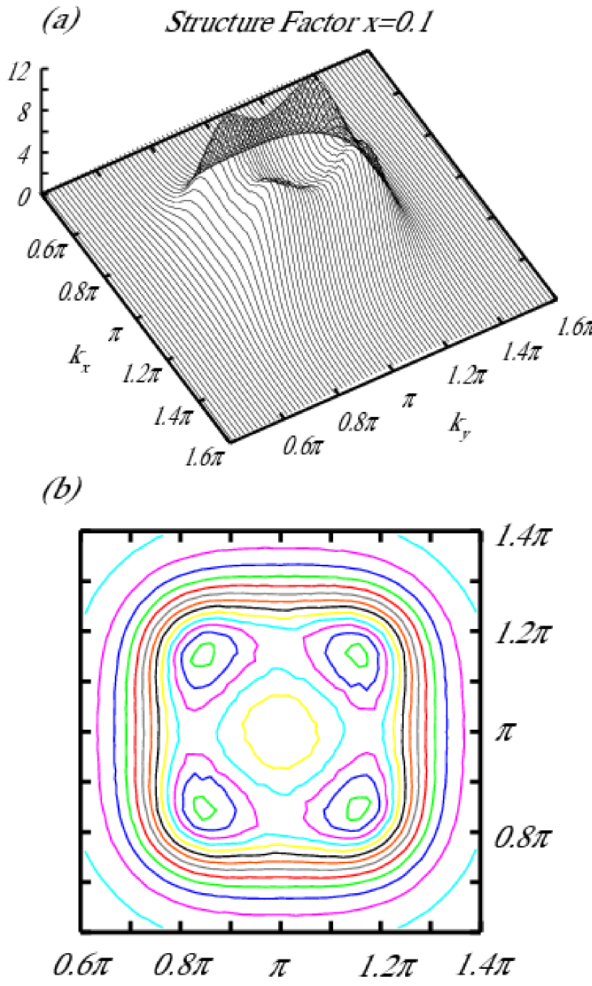
Figure 11: Static spin structure factor for $d^{9}$ spins at doping $x=0.10$. The structure factor is incommensurate with a ring of radius $k\approx(2\pi/a)x$ around $(\pi/a,\pi/a)$. The total sum over the Brillouin zone satisfies the normalization, $N^{-1}\sum_{k}S(k)=1$ where $N$ is the total number of cells. (a) 3D plot of structure factor. (b) contour plot centered at $(\pi/a,\pi/a)$.

Figures 11 and 12 show our results for the spin correlation at dopings $x=0.075$, $0.10$, and $0.125$ on a $256\times 256$ lattice averaged over an ensemble of $5,000$ configurations for each doping. The structure factor is dimensionless and is normalized such that its integral over the Brillouin zone is one, $N^{-1}\sum_{k}S(k)=1$, where $N$ is the total number of cells. Figure 13 shows part of a minimized spin structure at $x=0.10$.

Due to the large number of ensembles, the error bars for the plotted values are small. For $x=0.075$, they are $\pm 0.12$, $\pm 0.15$, and $\pm 0.12$ for the diagonal peak, $(\pi,\pi)$, and the Cu$-$O bond peak respectively. For $x=0.10$, the error is $\pm 0.09$, $\pm 0.08$, and $\pm 0.07$. For $x=0.125$, the error is $\pm 0.07$, $\pm 0.05$, and $\pm 0.05$. The error decreases sharply and becomes negligible on the scale of the figure as $k$ moves past the peaks and farther from $(\pi,\pi)$.

From figure 12, the diagonal incommensurate peak is shifted from $(\pi/a,\pi/a)$ by $(2\pi/a)(x/\sqrt{2})(1,1)$ and is of length $(2\pi/a)x$. The peak along the Cu$-$O bond direction is shifted in the range $(2\pi/a)x(1/\sqrt{2},0)$ to $(2\pi/a)x(1,0)$. The Cu$-$O bond direction shift is experimentally observed for the metallic range $x>0.05$ incommen_metal3 ; birgeneau_rmp in La_2-xSr_xCuO₄ and the diagonal shift is seen in the spin-glass regime $0.02<x<0.05$.incommensurate_sg

Since the difference between $(2\pi/a)x(1/\sqrt{2},0)$ and $(2\pi/a)x(1,0)$ is small, it is difficult to resolve the precise peak doping value within our finite size computations. If the structure factor derives from broadened Lorenztians centered at the four diagonal points around $(\pi/a,\pi/a)$, then a peak in the Cu$-$O bond direction would be expected at $(2\pi/a)x(1/\sqrt{2},0)$ from the two closest peaks. The contributions from the remaining two peaks shift the peak closer to $(\pi/a,\pi/a)$ rather than away from it as is seen in figure 12. Thus, the best we can currently say with the calculations is there is a ring of incommensurate peaks approximately a distance $k=(2\pi/a)x$ from $(\pi/a,\pi/a)$.

From the widths of the peaks, the correlation length is approximately the mean separation between the polarons, $a/\sqrt{x}$.

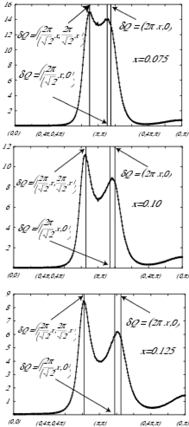
Figure 12: Static spin structure factor for $d^{9}$ spins at dopings $x=0.075$, $0.10$, and $0.125$ in La_2-xSr_xCuO₄. Each figure plots $S(k)$ starting from $k=(0,0)$ to $(\pi/a,\pi/a)$ and then to $(0,\pi/a)$. The structure factor is incommensurate with a ring of radius $k\approx(2\pi/a)x$ around $(\pi/a,\pi/a)$. The vertical lines are drawn to highlight specific incommensurate vectors. If the structure factor was purely derived from the sum of four Lorenztians along the diagonals a distance $(2\pi/a)x$ from $(\pi/a,\pi/a)$, then the peak along the Cu$-$O bond direction would be slightly less than the shift shown at $\delta Q=(2\pi/\sqrt{2}a,0)$. The normalization is the same as figure 11.

We present a heuristic derivation for why the spin structure factor is incommensurate with a shift from $(\pi/a,\pi/a)$ of magnitude $(2\pi/a)x$. Similar to previous work,gooding_birgeneau our calculations find that the minimum spin configuration consists of undoped patches of $d^{9}$ spins aligned antiferromagnetically with the polarons acting to rotate the direction of the antiferromagnetic alignment of adjacent patches. This is seen in figure 13.

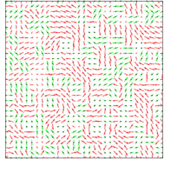
Figure 13: Projection of spins onto xy plane for an $x=0.10$ minimized structure. The $d^{9}$ spin staggered magnetization is along the z-axis out of the plane of the paper and the magnetization of the $d^{9}$ spins is along the x-axis. Only a $30\times 30$ subset of the $256\times 256$ lattice is shown. The undoped $d^{9}$ spins are shown in red and the polaron spins are green. The four Cu sites of each polaron are indicated by black dots.

Consider an area $A$. The number of polarons in this area is $N_{p}=Ax/a^{2}$. When the chiral coupling dominates, the effect of a single polaron on the neighboring $d^{9}$ spins is shown in figure 10. The polaron rotates each adjacent spin on opposite sides of the polaron by $\pi$, or $2\pi$ total. If this net $2\pi$ rotation is rigidly transmitted to an antiferromagnetic patch, then the polaron rotates a patch by an angle, $\delta\theta=2\pi/(1/x)=2\pi x$. Thus, the net rotation per spin is $N_{p}\delta\theta$. If the area $A$ is chosen such that the net rotation per spin is $2\pi$, or $N_{p}\delta\theta=2\pi$, then $A=(a/x)^{2}$. A translation by $L=\sqrt{A}=a/x$ returns to an identical antiferromagnetic patch. This leads to a shift of the spin correlation peak from $(\pi/a,\pi/a)$ to $\delta Q=2\pi/L$ or $\delta Q=(2\pi/a)x$.

V.3 Kinetic Energy of the $x^{2}-y^{2}$ Band

The energy contribution from the delocalized $x^{2}-y^{2}$ band electrons has not been included in the minimization of equation 48. A complete minimization would also compute the change in the band energy to determine the direction to align a given spin during our sweep through the lattice spins. This effect is included in mean-field below.

A $d^{9}$ spin ordering of momentum $\mathbf{q}$ hybridizes band electrons of momentum $\mathbf{k}$ and $\mathbf{k+q}$ with a coupling energy $V$ on the order of $J_{dd}\sim 0.1$ eV. This mixing of $\mathbf{k}$ and $\mathbf{k+q}$ perturbs the band energies and the total ground state energy. We calculate the band energy change in La_2-xSr_xCuO₄ for a ring of $\mathbf{q}$ vectors at the computed incommensurate length $q=(2\pi/a)x$. The $\mathbf{q}$ vector producing the lowest band energy is the observed neutron incommensurability.

The idea that the band kinetic energy change in the $d^{9}$ spin background determines the final neutron incommensurability has been suggested by Sushkov et al.kotov1 ; kotov2 ; kotov3 for the $t-t^{\prime}-t^{\prime\prime}-J$ model. In their model, the magnitude of the incommensurability arises from the doping $x$, the antiferromagnetic $d^{9}$ spin stiffness $\rho_{s}$, the hopping matrix element $t$, and the quasiparticle renormalization $Z$ where $q=(Zt/\rho_{s})(2\pi/a)x$. Their self-consistent Born approximation calculation of the quasiparticle dispersion in a spin-wave theory background finds values for the parameters such that $Zt/\rho_{s}\approx 1$. The magnitude of the incommensurability is less dependent on the detailed parameters for our Hamiltonian in equation 48.

For a given spin incommensurability vector $\mathbf{q}$ and $d^{9}$ to $x^{2}-y^{2}$ band coupling, $V\sim 0.1$ eV, the Green’s function satisfies,

$$G^{-1}(\mathbf{k},\omega) = G_{0}^{-1}(\mathbf{k},\omega)-V^{2}G_{0}(\mathbf{k+q},\omega)$$ (49)

$$- V^{2}G_{0}(\mathbf{k-q},\omega).$$

The vector $\mathbf{-q}$ must be included with $\mathbf{q}$ because the coupling Hamiltonian is Hermitean. Solving for $G(\mathbf{k},\omega)$,

$$G(\mathbf{k},\omega) = G_{0}(\mathbf{k},\omega)\left\{1-V^{2}G_{0}(\mathbf{k},\omega)\right.$$ (50)

$$\times \left.\left[G_{0}(\mathbf{k+q},\omega)+G_{0}(\mathbf{k-q},\omega)\right]\right\}^{-1}.$$

Expanding to order $V^{2}$,

$$G(\mathbf{k},\omega) = G_{0}(\mathbf{k},\omega)+V^{2}G_{0}(\mathbf{k},\omega)\left\{G_{0}(\mathbf{k+q},\omega)\right.$$ (51)

$$+ \left.G_{0}(\mathbf{k-q},\omega)\right\}G_{0}(\mathbf{k},\omega)$$

$$+ O(V^{4}).$$

The number of electrons in the $\mathbf{k}$ state up to energy $\epsilon$ is,

$$n(\mathbf{k},\epsilon)=\int_{-\infty}^{\epsilon}d\omega\left[-\frac{1}{\pi}\mathrm{Im}\ G(\mathbf{k},\omega)\right],$$ (52)

$$n(\mathbf{k},\epsilon) = n_{0}(\mathbf{k},\epsilon)+V^{2}\int_{-\infty}^{\epsilon}d\omega\left(-\frac{1}{\pi}\right)$$ (53)

$$\times \mathrm{Im}\left\{G_{0}(\mathbf{k},\omega)\left[G_{0}(\mathbf{k+q},\omega)\right.\right.$$

$$+ \left.\left.G_{0}(\mathbf{k-q},\omega)\right]G_{0}(\mathbf{k},\omega)\right\},$$

where $n_{0}(\mathbf{k},\epsilon)$ is the unperturbed occupation. The total density of states per spin at energy $\epsilon$ is,

$$N(\epsilon)=\sum_{\mathbf{k}}\left(-\frac{1}{\pi}\right)\mathrm{Im}\ G(\mathbf{k},\epsilon)=\frac{\partial}{\partial\epsilon}\sum_{\mathbf{k}}n(\mathbf{k},\epsilon),$$ (54)

A percolating band has Green’s function,

$$G_{0}(\mathbf{k},\omega)=\frac{1}{\omega-\epsilon_{k}+i\Gamma_{k}},\ \Gamma_{k}>0,$$ (55)

where $\Gamma_{k}$ is the linewidth. Using equations 52 and 55,

$$n_{0}(\mathbf{k},\omega)=\frac{1}{2}+\frac{1}{\pi}\tan^{-1}\left(\frac{\epsilon_{f}-\epsilon_{k}}{\Gamma_{k}}\right).$$ (56)

The perturbation shifts the Fermi level to $\epsilon_{f}+\delta\epsilon_{f}$. The total number of electrons is conserved, leading to the equation for $\delta\epsilon_{f}$,

$$n_{tot}=\sum_{\mathbf{k}}n(\mathbf{k},\epsilon_{f}+\delta\epsilon_{f})=\sum_{\mathbf{k}}n_{0}(\mathbf{k},\epsilon_{f}).$$ (57)

The total energy of the band electrons per spin is given by,

$$E_{tot}(\mathbf{q},V)=\int_{-\infty}^{\epsilon_{f}+\delta\epsilon_{f}}d\omega\ \omega\sum_{\mathbf{k}}n(\mathbf{k},\omega).$$ (58)

In appendix A, the expressions for $\delta\epsilon_{f}$ and $E_{tot}(\mathbf{q},V)$ to order $V^{2}$ are derived,

$$\delta\epsilon_{f}N_{0}(\epsilon_{f})+V^{2}\int_{-\infty}^{\epsilon_{f}}d\omega\sum_{\mathbf{k}}\left[R(\mathbf{k},\mathbf{k+q},\omega)\right.$$

$$+\left.R(\mathbf{k},\mathbf{k-q},\omega)\right]=0,$$ (59)

$$E_{tot}(\mathbf{q},V)=E_{G}+V^{2}\int_{-\infty}^{\epsilon_{f}}d\omega(\omega-\epsilon_{f})$$

$$\times\ \left[\sum_{\mathbf{k}}R(\mathbf{k},\mathbf{k+q},\omega)+R(\mathbf{k},\mathbf{k-q},\omega)\right],$$ (60)

where $N_{0}(\epsilon_{f})$ is the unperturbed density of states per spin, $E_{G}$ is the unperturbed $(V=0)$ energy, and

$$R(\mathbf{k},\mathbf{p},\omega) = \left(-\frac{1}{\pi}\right)\mathrm{Im}\left[\frac{1}{\left(\omega-\epsilon_{k}+i\Gamma_{k}\right)^{2}}\right.$$ (61)

$$\times \left.\frac{1}{\left(\omega-\epsilon_{p}+i\Gamma_{p}\right)}\right].$$

The integral $\int_{-\infty}^{\epsilon_{f}}R(\mathbf{k},\mathbf{p},\omega)d\omega$ can be evaluated analytically, thereby allowing us to accurately compute the small energy change of the Fermi energy $\delta\epsilon_{f}$ and $E_{tot}(\mathbf{q},V)$. This is done in appendix A.

The band energy is given by,

$$\begin{array}[]{ccc}\epsilon_{k}&=&-2t_{1}(\cos k_{x}+\cos k_{y})-4t_{11}\cos k_{x}\cos k_{y}\\ &&-2t_{2}(\cos 2k_{x}+\cos 2k_{y})+\epsilon_{x^{2}-y^{2}}.\\ \end{array}$$ (62)

We use the band structure parametersfreeman1 ; freeman2 ; kontani1 for La_2-xSr_xCuO₄ given by $t_{1}=0.25$ eV, $t_{11}=-0.025$ eV, and $t_{2}=0.025$ eV. $t_{1}$ is the nearest neighbor hopping, $t_{11}$ is the next-nearest neighbor diagonal term, and $t_{2}$ is the hopping along the Cu$-$O bond direction from two lattices site away. For $x=0.10$, $\epsilon_{x^{2}-y^{2}}=0.133$ eV leads to $\epsilon_{f}=0$.

We calculated the Fermi energy shift and energy for incommensurability along the diagonal and Cu$-$O bond direction of magnitude $q=(2\pi/a)x$ at $x=0.10$ with $V=0.1$ eV. The electron linewidth, $\Gamma_{k}$, is chosen to be the sum of an s-wave and d-wave term,

$$\Gamma_{k}=\Gamma_{S}+\Gamma_{D}(\cos k_{x}-\cos k_{y})^{2},$$ (63)

where $\Gamma_{S}=0.01$ eV and $\Gamma_{D}=0.01$ eV.

The addition of a d-wave term to the linewidth arises from the $\mathbf{k}$ dependence of the Coulomb scattering rate with polarons discussed in section VII.1.

The energy changes and Fermi level shifts in eV are,

$$\begin{array}[]{ccc}\delta E\left(\frac{2\pi x}{\sqrt{2}a},\frac{2\pi x}{\sqrt{2}a}\right)&=&-0.01456,\ \ \delta\epsilon_{f}=0.0046\\ \delta E\left(\frac{2\pi x}{a},0\right)&=&-0.01478,\ \ \delta\epsilon_{f}=-0.0056\\ \end{array}$$ (64)

The band energy is lower for incommensurability along the Cu$-$O bond direction.

The Cu$-$O bond direction incommensurability is lower in energy due to the additional Umklapp scattering available for $\mathbf{q}$ on the Brillouin zone edge rather than inside the zone for diagonal $\mathbf{q}$.

We have shown that chiral coupling of polarons to $d^{9}$ spins leads to a ring of incommensurability centered at $(\pi/a,\pi/a)$ of magnitude $(2\pi/a)x$. The perturbation to the kinetic energy of the delocalized $x^{2}-y^{2}$ band electrons selects incommensurability along the Cu$-$O bond direction due to Umklapp scattering on the Brillouin zone edge.

For $0.02<x<0.05$,birgeneau_rmp ; incommensurate_sg La_2-xSr_xCuO₄ is a spin-glass. No $x^{2}-y^{2}$ band is formed because the plaquette polarons do not percolate. The $x^{2}-y^{2}$ states triplet couple to polaron spins. The spin interactions in the spin-glass phase are different from the Hamiltonian in equation 48.

The Cu $x^{2}-y^{2}$ cannot delocalize over an infinite polaron swath in our model. We do not know if the $x^{2}-y^{2}$ states remain localized on a single Cu or delocalize over the finite swath of the polaron. Any delocalization leads to an effective ferromagnetic coupling between neighboring polaron spins due to the triplet coupling with the $x^{2}-y^{2}$ spin. In addition, there is an asymmetry in the chiral coupling due to orthorhombic crystal symmetry arising from the tilt of the CuO₆ octahedra. The one-dimensional incommensurability in the spin-glass phase of La_2-xSr_xCuO₄incommensurate_sg is not explained in this paper.

VI Superconducting Pairing

Coulomb scattering of $x^{2}-y^{2}$ band electrons with chiral plaquette polarons leads to anisotropic Cooper pair repulsion. The maximum energy difference between a chiral polaron and its time-reversed partner is analogous to the Debye energy in BCS superconductors, As discussed in section V.2, this energy difference can be non-zero and on the order of $J_{dd}$.

We simplify the polaron wavefunctions by absorbing the $p_{\sigma}$ orbitals into the A_1g orbitals on the Cu sites for the pairing and transport calculations. This is shown in figure 14.

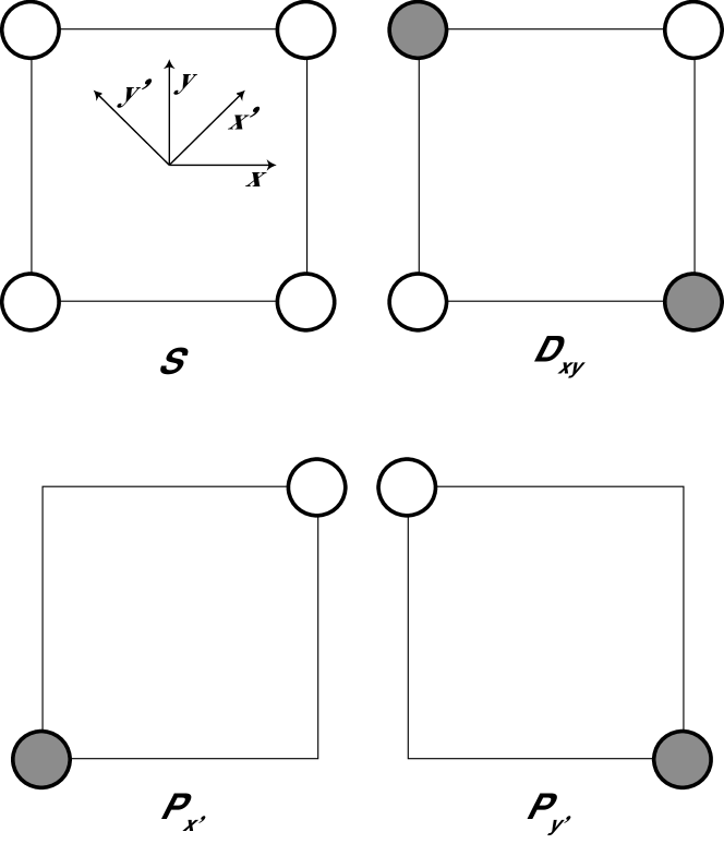
Figure 14: Effective polaron orbitals with $p_{\sigma}$ absorbed into A_1g on the Cu sites.

The direct and exchange Coulomb terms coupling the $x^{2}-y^{2}$ band with a polaron is,

$$H_{U}=U\sum_{\mathbf{R},\sigma,\sigma^{\prime}}d^{\dagger}_{R\sigma^{\prime}}z^{\dagger}_{R\sigma}z_{R\sigma}d_{R\sigma^{\prime}},$$ (65)

$$H_{K}=-K\sum_{\mathbf{R},\sigma,\sigma^{\prime}}d^{\dagger}_{R\sigma^{\prime}}z^{\dagger}_{R\sigma}z_{R\sigma^{\prime}}d_{R\sigma},$$ (66)

where $U>K>0$. $d^{\dagger}_{\mathbf{R}}$ creates an $x^{2}-y^{2}$ electron at $\mathbf{R}$ and $z^{\dagger}_{\mathbf{R}}$ creates an A_1g electron at $\mathbf{R}$.

The $x^{2}-y^{2}$ band state with momentum $\mathbf{k}$ is,

$$d^{\dagger}_{\mathbf{k}\sigma}=N^{-\frac{1}{2}}\sum_{\mathbf{R}}e^{i\mathbf{k}\cdot\mathbf{R}}d^{\dagger}_{\mathbf{R}\sigma},$$ (67)

where $N$ is the total number of Cu sites. A polaron state of spin $s$ is given by,

$$z^{\dagger}_{s}=\sum_{\mathbf{R}}\alpha_{\mathbf{R}}z^{\dagger}_{\mathbf{R}s},$$ (68)

where the coefficients $\alpha_{R}$ determine the type of polaron in figure 14. The matrix elements for direct and exchange Coulomb scattering of an $x^{2}-y^{2}$ band electron with a polaron electron are,

$$\left<k^{\prime}\sigma^{\prime},z_{s^{\prime}}|H_{U}|k\sigma,z_{s}\right>=\left(\frac{U}{N}\right)M(\mathbf{k^{\prime}-k})\delta_{\sigma\sigma^{\prime}}\delta_{ss^{\prime}},$$ (69)

$$\left<k^{\prime}\sigma^{\prime},z_{s^{\prime}}|H_{K}|k\sigma,z_{s}\right>=\left(-\frac{K}{N}\right)M(\mathbf{k^{\prime}-k})\delta_{\sigma s^{\prime}}\delta_{\sigma^{\prime}s},$$ (70)

$$M(\mathbf{q})=\sum_{\mathbf{R}}\alpha^{\prime\ast}_{\mathbf{R}}\alpha_{\mathbf{R}}e^{-i\mathbf{qR}}.$$ (71)

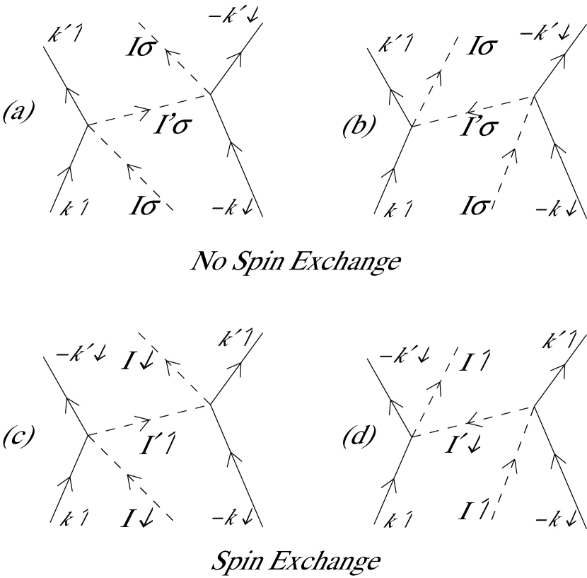
Figure 15: Second-order Cooper pairing processes with polarons. The Coulomb coupling is represented by a four-point vertex for simplicity. The solid lines are the band electrons and the dashed lines are the polaron states. $I$ is the initial and final polaron orbital state. $I^{\prime}$ is the intermediate state. (a) and (b) are the Coulomb couplings with no spin exchange. (c) and (d) are spin exchange couplings. In (c) and (d), the final electrons are interchanged compared to (a) and (b) yielding an extra minus sign in the pairing matrix element.

The Cooper pairing matrix element for scattering arising from figure 15(a) with initial polaron orbital state $I\uparrow$ is,

$$\left\langle(\mathbf{k^{\prime}}\uparrow,\mathbf{-k^{\prime}}\downarrow),I\uparrow\left|H^{\prime}\right|(\mathbf{k}\uparrow,\mathbf{-k}\downarrow),I\uparrow\right\rangle=$$

$$\frac{U(U-K)}{N^{2}}|M(\mathbf{q})|^{2}\sum_{I^{\prime}}\frac{1}{2}\left[\frac{1}{E_{f}-E_{n}}+\frac{1}{E_{i}-E_{n}}\right],$$ (72)

where $\mathbf{q=k^{\prime}-k}$, $E_{i}$ is the total energy of the initial state, $E_{f}$ is the final state energy, and $E_{n}$ is the intermediate state energy. The factor $U-K$ comes from the left vertex where both direct and exchange Coulomb matrix elements appear while the factor $U$ arises from the right vertex where there is no exchange. $E_{i}$, $E_{n}$, and $E_{f}$ are,

$$E_{i} = 2\epsilon_{k}+E_{I\uparrow},$$ (73)

$$E_{n} = \epsilon_{k}^{\prime}+\epsilon_{k}+E_{I^{\prime}\uparrow},$$ (74)

$$E_{f} = 2\epsilon_{k^{\prime}}+E_{I\uparrow}.$$ (75)

Substituting equations 73, 74, and 75 into VI leads to,

$$\left\langle(\mathbf{k^{\prime}}\uparrow,\mathbf{-k^{\prime}}\downarrow),I\uparrow\left|H^{\prime}\right|(\mathbf{k}\uparrow,\mathbf{-k}\downarrow),I\uparrow\right\rangle=$$

$$\frac{U(U-K)}{N^{2}}|M(\mathbf{q})|^{2}\sum_{I^{\prime}}\frac{\left(E_{I^{\prime}\uparrow}-E_{I\uparrow}\right)}{\left(\epsilon_{k^{\prime}}-\epsilon_{k}\right)^{2}-\left(E_{I^{\prime}\uparrow}-E_{I\uparrow}\right)^{2}}.$$ (76)

The pairing matrix element is the probability weighted average of equation VI over all initial polaron states $I$. States with $E_{I^{\prime}\sigma}-E_{I\sigma}>0$ dominate the average because the polaron is primarily in its lowest energy state. Since $U>0$ and $U-K>0$, there is an attractive pairing with momentum anisotropy determined by $|M(\mathbf{q})|^{2}$ for pairs close to the Fermi level. The coupling is attractive for Cooper pairs near the Fermi level within the polaron energy separation, $|\epsilon_{k}|$ and $|\epsilon_{k^{\prime}}|<\left(E_{I^{\prime}\sigma}-E_{I\sigma}\right)$. There are similar terms for $I\downarrow$ and figure 15(b).

For the spin exchange processes shown in figures 15(c) and (d), the matrix element picks up an extra minus sign compared to figures 15(a) and (b) due to the exchange of $\mathbf{k^{\prime}}\uparrow$ and $\mathbf{-k^{\prime}}\downarrow$ in the final state,

$$\left\langle(\mathbf{k^{\prime}}\uparrow,\mathbf{-k^{\prime}}\downarrow),I\sigma\left|H^{\prime\prime}\right|(\mathbf{k}\uparrow,\mathbf{-k}\downarrow),I\sigma\right\rangle=$$

$$(-)\left(\frac{-K}{N}\right)^{2}|M(\mathbf{k^{\prime}+k})|^{2}\sum_{I^{\prime}}\frac{\Delta}{\left(\epsilon_{k^{\prime}}-\epsilon_{k}\right)^{2}-\Delta^{2}},$$ (77)

where $\Delta=E_{I^{\prime}\uparrow}-E_{I\downarrow}$. This leads to an overall repulsive interaction for pairs near the Fermi level.

The direct on-site isotropic Coulomb repulsion between Cooper pairs must be included in the net pairing interaction in addition to the second-order pairings in figure 15.

For hole-doped cuprates, one chiral polaron state is singly occupied and the remaining polaron states shown in figure 3 are doubly occupied. The intermediate polaron state $I^{\prime}$ must be a chiral state, $P_{x^{\prime}}\pm iP_{y^{\prime}}$. For electron-doped cuprates, the initial state $I$ is a chiral polaron. The pairing is identical because the matrix element between $I$ and $I^{\prime}$ is mod-squared. We focus on the hole-doped derivation here.

The momentum dependence of the pairing is determined by $|M(\mathbf{q})|^{2}$ where $\mathbf{q=k^{\prime}-k}$ for non-spin exchange attraction and $\mathbf{q=k^{\prime}+k}$ for spin exchange repulsion. $|M(\mathbf{q})|^{2}$ is the same for $I=S$ and $D_{xy}$. From figure 14 and equation 71,

$$|M(\mathbf{q})|^{2}_{S,D}\sim\sin^{2}\frac{1}{2}\left(q_{x}+q_{y}\right)+\sin^{2}\frac{1}{2}\left(-q_{x}+q_{y}\right),$$ (78)

where we have dropped all constants and wavefunction normalizations in the expression because they do not affect the momentum dependence. For $I=P_{x^{\prime}}\pm iP_{y^{\prime}}$ and $I^{\prime}=P_{x^{\prime}}\mp iP_{y^{\prime}}$,

$$|M(\mathbf{q})|^{2}_{+-}\sim\left[\cos\frac{1}{2}\left(q_{x}+q_{y}\right)-\cos\frac{1}{2}\left(-q_{x}+q_{y}\right)\right]^{2}.$$ (79)

For spin exchange repulsion, there is an additional possibility where $I^{\prime}=I=P_{x^{\prime}}\pm iP_{y^{\prime}}$. $|M(\mathbf{q})|^{2}_{++}$ is,

$$|M(\mathbf{q})|^{2}_{++}\sim\left[\cos\frac{1}{2}\left(q_{x}+q_{y}\right)+\cos\frac{1}{2}\left(-q_{x}+q_{y}\right)\right]^{2}.$$ (80)

Table 4 shows the value of $|M(\mathbf{q})|^{2}$ for various vectors $\mathbf{q}$. There are several pairing possibilities.

First, consider non-spin exchange attractive pairing through figures 15(a) and (b) added to direct isotropic repulsion. In this case, $\mathbf{q=k^{\prime}-k}$. $|M(\mathbf{q})|^{2}_{S,D}$ leads to a net attraction for $\mathbf{q}=(\pi,0)$. An s-wave gap cannot occur because the isotropic repulsion dominates. A gap of any other symmetry has a net repulsion for $\mathbf{q}=(0,0)$ and cannot lead to superconductivity. $|M(\mathbf{q})|^{2}_{+-}$ also repels at $\mathbf{q}=(0,0)$ and does not superconduct. $M_{++}$ does not occur for non-spin exchange. Thus, there is no superconductivity through non-spin exchange polaron coupling.

Table 4: The values of $|M(q)|^{2}$ at special vectors in the Brillouin zone. For non-spin exchange couplings shown in figure 15(a) and (b), the last column does not apply because the intermediate cannot be identical to the initial polaron state, $I^{\prime}\neq I$. $M(q)$ is defined in equations 78, 79, and 80. $\mathbf{q=k^{\prime}\mp k}$ for non-spin exchange and spin exchange respectively.

$(q_{x},q_{y})$	$|M(q)|^{2}_{S,D}$	$|M(q)|^{2}_{+-}$	$|M(q)|^{2}_{++}$
$(0,0)$	0	0	4
$(\pi,0)$, $(0,\pi)$	2	0	0
$(\pi,\pi)$	0	4	0

For spin exchange repulsion in figures 15(c) and (d) added to direct isotropic repulsion, $M_{S,D}$ has the largest repulsion for $\mathbf{q=k^{\prime}+k}=(\pi,0)$, $M_{+-}$ for $\mathbf{q}=(\pi,\pi)$, and $M_{++}$ for $\mathbf{q}=(0,0)$. $M_{++}$ cannot be correct for the cuprates because $\mathbf{q}=0$ when $\mathbf{k^{\prime}=-k}$. This leads to a gap that changes sign for $\mathbf{k}\rightarrow\mathbf{-k}$ and triplet spin pairing. For $M_{S,D}$, there is no favorable Fermi surface nesting near $\mathbf{k^{\prime}+k}=(\pi,0)$.

$M_{+-}$ has the time-reversed chiral polaron as the intermediate state and has a large repulsion for $\mathbf{k^{\prime}+k}=(\pi,\pi)$. For $\mathbf{k}\approx(\pi,0)$ and $\mathbf{k^{\prime}}\approx(0,\pi)$, there is a large repulsion between pairs close to the Fermi surface. Pairing through spin exchange coupling with time-reversed polarons leads to d-wave superconductivity.

As discussed in section V.2 on the neutron spin incommensurability, the energy splitting between time-reversed chiral polarons is on the scale of $J_{dd}\sim 0.1$ eV. It is this scale that is analogous to the phonon Debye energy in conventional superconductors.

The energy separation between two time-reversed chiral polarons, $|P_{x^{\prime}}+iP_{y^{\prime}},\sigma\rangle$ and $|P_{x^{\prime}}-iP_{y^{\prime}},-\sigma\rangle$, is largest for low dopings where there are more undoped $d^{9}$ spins. The energy splitting decreases with increasing doping leading to a reduction in the energy range surrounding the Fermi surface involved in Cooper pairing. Concurrently, the number of polarons that can induce Cooper pairing increases. The number of band $x^{2}-y^{2}$ electrons available to form the superconducting ground state also increases with increasing doping. Finally, as the number of polarons increases, they crowd into each other, eventually creating polarons localized on single Cu sites, as found in UB3LYP calculationsub3lyp_dope . The single Cu state is not chiral and leads to isotropic Cooper pair repulsion. The competition between all of these factors leads to the superconducting phase diagram in cuprates.

VII Normal State Transport

VII.1 Resistivity

The temperature dependence of the resistivity arising from $x^{2}-y^{2}$ band electrons Coulomb scattering from polarons is shown to depend on the density of polaron energy separations, $\rho(\Delta)$. If the density is constant, then the resistivity is linear in $T$.

The scattering rate of an $x^{2}-y^{2}$ electron initially in the state $\mathbf{k}\sigma$ to Coulomb scatter from a polaron to another band electron and polaron is the sum,

$$\frac{1}{\tau(\epsilon_{k\sigma})} = \frac{2\pi}{\hbar}\sum_{\stackrel{{\scriptstyle\mathbf{k^{\prime}}\sigma^{\prime}}}{{Is,I^{\prime}s^{\prime}}}}|\langle\mathbf{k^{\prime}\sigma^{\prime}},I^{\prime}s^{\prime}|H^{\prime}|\mathbf{k\sigma},Is\rangle|^{2}P(Is)$$ (81)

$$\times\ \delta(\epsilon_{\mathbf{k^{\prime}\sigma^{\prime}}}+E_{I^{\prime}s^{\prime}}-\epsilon_{\mathbf{k\sigma}}-E_{Is}),$$

where $H^{\prime}=H_{U}+H_{K}$ is the total Coulomb interaction of band electrons with polarons. $H_{U}$ and $H_{K}$ are defined in equations 65 and 66. $E_{Is}$ and $E_{I^{\prime}s^{\prime}}$ are the initial and final polaron energies respectively. $P(Is)$ is the probability the polaron is initially in the state $Is$. The delta function enforces total energy conservation,

$$\epsilon_{\mathbf{k\sigma}}+E_{Is}=\epsilon_{\mathbf{k^{\prime}\sigma^{\prime}}}+E_{I^{\prime}s^{\prime}}.$$ (82)

The matrix element in equation 81 is proportional to $|M(\mathbf{k^{\prime}-k})|^{2}$ defined in equations 78, 79, and 80. To obtain the qualitative temperature dependence, we simplify equation 81 by assuming the matrix element is constant for all momenta and there are only two polaron states at any doped center. This does not alter the temperature dependence, but smears out the anisotropy of the scattering rate. The $M(\mathbf{k^{\prime}-k})$ have different momentum dependencies for each polaron symmetry. Since the scattering rate is a sum over all scattering channels, the approximation of isotropic scattering is likely to be good.

There is a polaron Coulomb scattering process we have neglected. This is second-order hopping of a $\mathbf{k}$ $x^{2}-y^{2}$ electron into the unoccupied polaron state that then hops off into a $\mathbf{k^{\prime}}$ $x^{2}-y^{2}$ band state. Since the polaron is comprised of orbitals with A₁ symmetry, the hopping is zero for momenta along the zone diagonal and largest at $(\pm\pi,0)$ and $(0,\pm\pi)$. This term is approximately temperature independent and of “d-wave” symmetry. The temperature dependence of this term arises from the displacement of the apical O due to the addition of an electron into the polaron. Since the initial and final states in this second-order process have one hole on the polaron, the temperature dependence is expected to be weak. We neglect this additive temperature independent anisotropic constant term in the remainder of this section.

The neglected term justifies the addition of a d-wave lifetime broadening of the band electrons for the computation of the change in the band energy from the neutron spin incommensurability in section V.3.

Consider an $x^{2}-y^{2}$ band electron with energy $\epsilon_{1}$ and a polaron with energy $E_{i}$ scattering to an electron with energy $\epsilon_{2}$ and polaron with energy $E_{f}$. $\epsilon_{1}$ and $\epsilon_{2}$ are measured relative to the Fermi level, $\epsilon_{f}=0$. Conservation of energy is,

$$\epsilon_{1}=\epsilon_{2}+\Delta,\ \ \Delta\equiv E_{f}-E_{i}.$$ (83)

The thermal occupations of a doped site with two polaron states of energy $E_{i}$ and $E_{f}$ is given by the Fermi-Dirac functions $f(-\Delta)$ and $f(\Delta)$ defined in equation 28 and depends only on the energy difference $\Delta$. This is identical to the results in equation 27.

The total lifetime of a band state with energy $\epsilon_{1}$ is given by,

$$\frac{1}{\tau(\epsilon_{1})} = \int d\epsilon_{2}\int d\Delta\ \rho(\Delta)\frac{2\pi}{\hbar}|H^{\prime}|^{2}$$ (84)

$$\times \delta(\epsilon_{2}-\epsilon_{1}-\Delta)f(-\Delta)\left[1-f(\epsilon_{2})\right],$$

where $\rho(\Delta)$ is the density of polaron sites with an energy splitting $\Delta$ and $|H^{\prime}|^{2}$ is taken to be a constant. The $\rho(\Delta)$ used here is different from the spin and chirality flipped density in section V.1. $\rho(\Delta)$ in equation 84 includes the energy splittings of the $S$, $D_{xy}$, and the bonding combinations of the $P_{x^{\prime}}$ and $P_{y^{\prime}}$ polaron states.

Integrating over the final electron energy $\epsilon_{2}$,

$$\frac{1}{\tau(\epsilon_{1})} = \frac{2\pi}{\hbar}|H^{\prime}|^{2}N(0)$$ (85)

$$\times \int d\Delta\ \rho(\Delta)f(-\Delta)\left[1-f(\epsilon_{1}-\Delta)\right],$$

where $N(0)$ is the band density of states per spin.

For $\epsilon_{1}$ at the Fermi level, $\epsilon_{1}=0$, the integrand becomes $\rho(\Delta)f(\Delta)[1-f(\Delta)]$ leading to a temperature dependence $T^{\mu+1}$ if $\rho(\Delta)\sim\Delta^{\mu}$. For a uniform distribution of polaron energy splittings, $\rho(\Delta)=\rho_{0}$ for $|\Delta|\leq\Delta_{max}$ and zero otherwise, the integral in equation 85 is,

$$\frac{1}{\tau(\epsilon_{1})} = \frac{2\pi}{\hbar}|H^{\prime}|^{2}N(0)\rho_{0}$$ (86)

$$\times \frac{T}{\left(1-e^{-\beta\epsilon_{1}}\right)}\ln\left[\frac{e^{\beta\Delta_{max}}+e^{-\beta\epsilon_{1}}}{e^{\beta(\Delta_{max}-\epsilon_{1})}+1}\right].$$

The energy scale for $\Delta_{max}$ is determined by the scale for the hopping matrix elements and is several tenths of an eV. This is much larger than the temperature, $\beta\Delta_{max}\gg 1$. For $|\epsilon_{1}|\ll\Delta_{max}$, we may take the limit $\Delta_{max}\rightarrow+\infty$ leading to,

$$\frac{1}{\tau(\epsilon_{1})}=\frac{2\pi}{\hbar}|H^{\prime}|^{2}N(0)\rho_{0}\left(\frac{\epsilon_{1}}{1-e^{-\beta\epsilon_{1}}}\right).$$ (87)

The $\tau_{B}$ that appears in the Boltzmann transport equation is related to the linewidth and satisfies,

$$\frac{1}{\tau_{B}(\epsilon_{1})}=-\frac{2}{\hbar}\mathrm{Im}\ \Sigma(\epsilon_{1})=\frac{1}{\tau(\epsilon_{1})}\cdot\frac{1}{1-f(\epsilon_{1})},$$ (88)

$$\frac{1}{\tau_{B}(\epsilon)}=\frac{2\pi}{\hbar}|H^{\prime}|^{2}N(0)\rho_{0}\ \epsilon\coth\frac{1}{2}\beta\epsilon.$$ (89)

At the Fermi level, $\epsilon=0$, the scattering rate is,

$$\frac{1}{\tau_{B}(\epsilon)}=\frac{2\pi}{\hbar}|H^{\prime}|^{2}N(0)\rho_{0}(2T),$$ (90)

leading to a linear resistivity.

If $\rho(\Delta)\sim\Delta$ for $|\Delta|\leq\Delta_{min}$ and is constant for $\Delta_{min}\leq\Delta\leq\Delta_{max}$, then the resistivity is $\sim T^{2}$ at low temperature and crosses over to $\sim T$ at high temperature. Different forms for $\rho(\Delta)$ lead to different temperature dependencies for the resistivity as seen in La_2-xSr_xCuO₄ from $0.05<x<0.35$. cava_resist

The optical spectrum is composed of a Drude scattering term for finite $\epsilon$ in equations 86 and 89 plus polaron to polaron scattering due to photon absorption. The Drude scattering rate becomes proportional to $\epsilon$ for $\beta\epsilon\gg 1$ with the crossover from $T$ to $\epsilon$ occurring when $\beta\epsilon\approx 2$. When the energy is larger than the largest polaron splitting, $\epsilon\gg\Delta_{max}$ the scattering rate saturates and becomes proportional to $\Delta_{max}$.

Direct optical absorption from $S$ and $D_{xy}$ polarons to $P_{x^{\prime}}\pm iP_{y^{\prime}}$ can occur for light polarized in the CuO₂ planes. This leads to the excess mid-IR absorption. optics1

Chiral polarons can lead to the logarithmic resistivity upturn at low temperatures due to a Kondo effect. boeb1 As La_2-xSr_xCuO₄ is doped, polaron islands are formed composed of exactly one polaron with no adjacent polarons. Island polarons are surrounded by $d^{9}$ spins. They have two possible chiral ground states. Antiferromagnetic spin flip scattering with the $x^{2}-y^{2}$ band occurs in second-order where the $x^{2}-y^{2}$ electron hops onto the polaron and either an up or down spin polaron hops back to the $x^{2}-y^{2}$ band. This leads to a Kondo effect.

The momentum dependence of the antiferromagnetic Kondo spin exchange is largest for momenta near $(\pm\pi,0)$ and $(0,\pm\pi)$ since the polaron is comprised of A₁ orbitals. The coupling is zero for momenta along the diagonal. The resistivity in the plane is dominated by electrons with momentum near the diagonals and transport out of the plane by momenta near $(\pm\pi,0)$ and $(0,\pm\pi)$. The resistivity upturn due to Kondo scattering appears at a higher temperature for out of plane transport.

There is no Kondo effect from Coulomb scattering with polarons from $H_{U}+H_{K}$ defined in equations 65 and 66 because the spin coupling is ferromagnetic.

Figure 16 shows the number of islands per unit cell as a function of doping for a 2D lattice with doped polarons. The Kondo resistivity is expected to disappear as the number of islands goes to zero. From table 3, the polarons percolate in 2D at $x\approx 0.15$. This is approximately the doping where the insulator to metal transition occurs for La_2-xSr_xCuO₄.boeb1

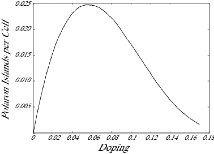
Figure 16: Number of polaron islands per Cu as a function of doping for a 2D Cu lattice. An island is defined as a four-site polaron having only undoped $d^{9}$ spins as neighbors.

The above suggestion has several caveats that could invalidate the conclusion. First, we do not know how many islands exist with a small energy separation between the chiral polaron time-reversed states.

Second, the g-factor for these islands needs to be evaluated to determine the energy splitting between the “up” and “down” states. The Kondo effect is suppressed for temperatures less than the splitting energy. 60 Tesla pulsed magnetic fields were used to suppress the superconductivity in order to access the low temperature normal state.boeb1

The g-factor of an electron spin is two, $g_{e}=2$. A 60 Tesla field splits the up and down electron spin energies by 80K. For $g=0.1$, the splitting is 4K. The Kondo effect is active for $T>4$K.

An estimate of the polaron g-factor, $g_{p}$, is made in section VII.2 by fitting to the temperature dependent Hall effect for La_2-xSr_xCuO₄ at $x=0.10$. It is argued that $g_{p}\sim 0.1$. Also, for island polarons, figure 10 shows the energy difference between a polaron and time-reversed polaron is zero for large $J_{ch}$. This order of magnitude reduction in $g_{p}$ allows the Kondo effect to remain active at low temperatures.

Third, the coupling to the band electrons needs to be evaluated to determine if the logarithmic resistivity is of the right magnitude.

VII.2 Hall Effect

Skew-scattering has been proposedvarma1 to explain the temperature dependence of the Hall effect although the physical nature of the excitations causing the skew-scattering was unclear. In this section, we derive and estimate the magnitude and temperature dependence of the skew-scattering of $x^{2}-y^{2}$ band electrons from chiral plaquette polarons. The skew-scattering contribution to the Hall effect is an extra term that is added to the ordinary Hall effect.

Skew-scatteringfert1 ; fert2 ; fert3 ; coleman1 ; skew_boltz1 ; skew_boltz2 is a left-right scattering asymmetry occurring when the scattering rate from $\mathbf{k\rightarrow k^{\prime}}$ is not equal to the scattering rate from $\mathbf{k^{\prime}\rightarrow k}$, $w(\mathbf{k\rightarrow k^{\prime}})\neq w(\mathbf{k^{\prime}\rightarrow k})$. A combination of time-reversal and inversion symmetry leads to no skew-scattering because $w(\mathbf{k\rightarrow k^{\prime}})=w(\mathbf{-k\rightarrow-k^{\prime}})$ due to inversion and $w(\mathbf{-k\rightarrow-k^{\prime}})=w(\mathbf{k^{\prime}\rightarrow k})$ from time-reversal invariance. An applied magnetic field breaks time-reversal invariance by making the number of polarons of “up” and “down” chirality different.

Skew-scattering first appears in third order for the scattering Hamilitonian as can be seen in the simple example below where we ignore the polarons and consider a band scattering matrix element that is complex.

Let $H^{\prime}$ be the electron scattering Hamiltonian,

$$H^{\prime}=\sum_{\mathbf{k,k^{\prime}}\sigma}V_{\mathbf{k^{\prime}k}}d^{\dagger}_{\mathbf{k^{\prime}}\sigma}d_{\mathbf{k}\sigma},$$ (91)

where we ignore any spin dependence in the matrix element $V_{\mathbf{kk^{\prime}}}$. Since $H^{\prime}$ is Hermitean, $V_{\mathbf{k^{\prime}k}}=V^{\ast}_{\mathbf{kk^{\prime}}}$. The scattering $T$ matrix is given by

$$T(E)=V+VG(E)V+\cdots,$$ (92)

and the scattering rate is,

$$w(\mathbf{k\rightarrow k^{\prime}})=\frac{2\pi}{\hbar}|\langle\mathbf{k^{\prime}}|T(\epsilon_{k})|\mathbf{k}\rangle|^{2}\delta(\epsilon_{k^{\prime}}-\epsilon_{k}).$$ (93)

Expanding the $T$ matrix to second-order,

$$\langle\mathbf{k^{\prime}}|T(\epsilon_{k})|\mathbf{k}\rangle=V_{\mathbf{k^{\prime}k}}+\sum_{\mathbf{k^{\prime\prime}}}\frac{V_{\mathbf{k^{\prime}k^{\prime\prime}}}V_{\mathbf{k^{\prime\prime}k}}}{\epsilon_{k}-\epsilon_{k^{\prime}}+i\delta}+O(V^{3}).$$ (94)

Substituting into equation 93 and neglecting terms of $O(V^{4})$,

$$w(\mathbf{k\rightarrow k^{\prime}})=\frac{2\pi}{\hbar}\left[|V_{\mathbf{k^{\prime}k}}|^{2}+\sum_{\mathbf{k^{\prime\prime}}}\frac{2\mathrm{Re}(V_{\mathbf{k^{\prime}k}}V_{\mathbf{kk^{\prime\prime}}}V_{\mathbf{k^{\prime\prime}k^{\prime}}})}{\epsilon_{k}-\epsilon_{k^{\prime\prime}}}\right.$$

$$\left.-2\pi\sum_{\mathbf{k^{\prime\prime}}}\mathrm{Im}(V_{\mathbf{k^{\prime}k}}V_{\mathbf{kk^{\prime\prime}}}V_{\mathbf{k^{\prime\prime}k^{\prime}}})\delta(\epsilon_{k}-\epsilon_{k^{\prime\prime}})\right]\delta(\epsilon_{k}-\epsilon_{k^{\prime}}).\ \$$ (95)

As a check, equation VII.2 is invariant under any redefinition of the $\mathbf{k}$ states, $V_{\mathbf{k^{\prime}k}}\rightarrow e^{i(\theta_{\mathbf{k^{\prime}}}-\theta_{\mathbf{k}})}V_{\mathbf{k^{\prime}k}}$.

If $V$ is real, then there is no skew-scattering since $w(\mathbf{k\rightarrow k^{\prime}})=w(\mathbf{k^{\prime}\rightarrow k})$. If $V$ is complex, then interchanging $\mathbf{k}$ and $\mathbf{k^{\prime}}$ changes the sign of the third term. This is the lowest order skew-scattering term. By interchanging $\mathbf{k^{\prime}\leftrightarrow k^{\prime\prime}}$ in the third term of the equation, the sum over $\mathbf{k^{\prime}}$ of the skew term satisfies $\sum_{k^{\prime}}w_{skew}(\mathbf{k\rightarrow k^{\prime}})=0$.

The applied magnetic field causes skew-scattering by creating left-right asymmetries. The relevant question is not if there is any skew scattering, but whether the scattering is large enough to account for the experimental Hall effect and its temperature dependence.

We derive the skew-scattering from the Coulomb Hamiltonian $H_{U}$ in equation 65. Including the exchange term $H_{K}$ in equation 66 does not change the results below because it leads to an average over $U$ and $U-K$. Thus, we focus on $H_{U}$ and ignore the electron spin.

Consider a single polaron. In the hole-doped cuprates, one of the chiral polaron states, $P^{\pm}\equiv P_{x^{\prime}}\pm iP_{y^{\prime}}$ is initially unoccupied and all the remaining polaron states shown in figure 14 are occupied. The matrix elements for scattering an $x^{2}-y^{2}$ $\mathbf{k}$ electron and polaron electron to a chiral polaron state with a change in the $x^{2}-y^{2}$ band electron momentum to $\mathbf{k^{\prime}}$ is,

$$\langle\mathbf{k^{\prime}}P^{\pm}|H_{U}|\mathbf{k}S\rangle=\left(\frac{U}{2N}\right)(-i)\left(\sin q_{x^{\prime}}\mp i\sin q_{y^{\prime}}\right),$$ (96)

$$\langle\mathbf{k^{\prime}}P^{\pm}|H_{U}|\mathbf{k}D_{xy}\rangle=\left(\frac{U}{2N}\right)(-i)\left(\sin q_{x^{\prime}}\pm i\sin q_{y^{\prime}}\right),$$ (97)

$$\langle\mathbf{k^{\prime}}P^{\pm}|H_{U}|\mathbf{k}P^{\pm}\rangle = \left(\frac{U}{2N}\right)\left(\cos q_{x^{\prime}}+\cos q_{y^{\prime}}\right),$$ (98)

$$= \left(\frac{U}{N}\right)\cos\frac{1}{2}q_{x}\cos\frac{1}{2}q_{y},$$ (99)

$$\langle\mathbf{k^{\prime}}P^{\pm}|H_{U}|\mathbf{k}P^{\mp}\rangle = \left(\frac{U}{2N}\right)\left(\cos q_{x^{\prime}}-\cos q_{y^{\prime}}\right),$$ (100)

$$= (-)\left(\frac{U}{N}\right)\sin\frac{1}{2}q_{x}\sin\frac{1}{2}q_{y},$$ (101)

where $\mathbf{q=k^{\prime}-k}$ and

$$q_{x^{\prime}} = \frac{1}{2}\left(q_{x}+q_{y}\right),$$ (102)

$$q_{y^{\prime}} = \frac{1}{2}\left(-q_{x}+q_{y}\right).$$ (103)

The chiral polaron to chiral polaron scattering terms in equations 99 and 101 are real and lead to no skew-scattering, as shown below. Second-order mixing with $S$ and $D_{xy}$ polaron symmetries leads to skew-scattering.

The Coulomb repulsion, $U$, in the above matrix elements is positive, $U>0$. The matrix elements corresponding to equations 96$-$101 for hole polarons are obtained by the substitution $U\rightarrow-U$. We use the expressions in equations 96$-$101 and remember to take $U<0$ for the hole-doped materials and $U>0$ for the electron-doped materials.

The $T$ matrix element is defined as,

$$T^{\pm}_{\mathbf{k^{\prime}k}}=\langle\mathbf{k^{\prime}}P^{\pm}|T|\mathbf{k}P^{\pm}\rangle,$$ (104)

where the hole resides in $P^{\pm}$ (the electron is in $P^{\mp}$). Expanding $T^{\pm}_{\mathbf{k^{\prime}k}}$ to order $U^{2}$,

$$T^{\pm}_{\mathbf{k^{\prime}k}}=V^{(1)}_{\mathbf{k^{\prime}k}}+\sum_{I}V^{(2)(\pm)}_{\mathbf{k^{\prime}k}}(I)+O(U^{3}),$$ (105)

where the sum is over all intermediate polaron states $I$. $V^{(1)}_{\mathbf{k^{\prime}k}}$ is defined as,

$$V^{(1)}_{\mathbf{k^{\prime}k}}=\langle\mathbf{k^{\prime}}P^{\pm}|H_{U}|\mathbf{k}P^{\pm}\rangle,$$ (106)

and is independent of the polaron chirality and real from equation 99. Thus, $V^{(1)}_{\mathbf{k^{\prime}k}}=V^{(1)}_{\mathbf{kk^{\prime}}}$. $V^{(2)}$ is,

$$V^{(2)(\pm)}_{\mathbf{k^{\prime}k}}=\sum_{\mathbf{p}}\frac{\langle\mathbf{k^{\prime}}P^{\pm}|H_{U}|\mathbf{p}I\rangle\langle\mathbf{p}I|H_{U}|\mathbf{k}P^{\pm}\rangle}{\epsilon_{k}-\epsilon_{p}-\left(E_{I}-E^{\pm}\right)+i\delta},$$ (107)

where the sum is over all intermediate $x^{2}-y^{2}$ momenta $\mathbf{p}$. $E^{\pm}$ and $E_{I}$ are the chiral polaron and the intermediate polaron energies respectively. $\epsilon_{p}$ is the $x^{2}-y^{2}$ band energy for momentum $\mathbf{p}$.

Since $V^{(1)}$ is real, $|T^{\pm}_{\mathbf{k^{\prime}k}}|^{2}$ is,

$$|T^{\pm}_{\mathbf{k^{\prime}k}}|^{2}=\left(V^{(1)}_{\mathbf{k^{\prime}k}}\right)^{2}+V^{(1)}_{\mathbf{k^{\prime}k}}\sum_{I}2\mathrm{Re}V^{(2)(\pm)}_{\mathbf{k^{\prime}k}}(I)+O(U^{3}).$$ (108)

The skew-scattering contribution is antisymmetric under interchange, $\mathbf{k^{\prime}\leftrightarrow k}$. The first term in equation 108 is symmetric and so is $V^{(2)(\pm)}_{\mathbf{k^{\prime}k}}(I)$ for $I=P^{\pm}$. The lowest order skew-scattering term is,

$$|T^{\pm}_{\mathbf{k^{\prime}k}}|^{2}_{s}=V^{(1)}_{\mathbf{k^{\prime}k}}\cdot 2\mathrm{Re}\left[V^{(2)(\pm)}_{\mathbf{k^{\prime}k}}(S)+V^{(2)(\pm)}_{\mathbf{k^{\prime}k}}(D_{xy})\right].$$ (109)

In appendix B, it is shown the antisymmetric terms in $V^{(2)(\pm)}(S,D_{xy})$ are,

$$\mathrm{Re}V^{(2)(\pm)}_{\mathbf{k^{\prime}k}}(S)=\mp\left(\frac{U^{2}}{4N}\right)\pi F_{1}\left[\epsilon_{k}-(E_{S}-E^{\pm})\right]A_{\mathbf{k^{\prime}},\mathbf{k}},$$ (110)

$$\mathrm{Re}V^{(2\pm)}_{\mathbf{k^{\prime}k}}(D)=\pm\left(\frac{U^{2}}{4N}\right)\pi F_{1}\left[\epsilon_{k}-(E_{D}-E^{\pm})\right]A_{\mathbf{k^{\prime}},\mathbf{k}},$$ (111)

where the antisymmetric function, $A_{\mathbf{kk^{\prime}}}=-A_{\mathbf{k^{\prime}k}}$, is,

$$A_{\mathbf{k^{\prime}},\mathbf{k}}=\sin k_{x^{\prime}}\sin k^{\prime}_{y^{\prime}}-\sin k_{y^{\prime}}\sin k^{\prime}_{x^{\prime}}.$$ (112)

Equations 102 and 103 define the $x^{\prime}$ and $y^{\prime}$ components of $\mathbf{k}$ and $\mathbf{k^{\prime}}$. The function $F_{1}$ is the sum over the Brillouin zone,

$$F_{1}(\omega)=\frac{1}{N}\sum_{\mathbf{p}}\frac{1}{2}\left(\cos p_{x}+\cos p_{y}\right)\delta(\omega-\epsilon_{p}).$$ (113)

The $D_{xy}$ contribution is negative the $S$ contribution with $E_{D}$ substituted for $E_{S}$.

The skew-scattering term is,

$$|T^{\pm}_{\mathbf{k^{\prime}k}}|^{2}_{s} = \mp\left(\frac{1}{N^{2}}\right)U^{3}\left(\frac{\pi}{2}\right)\cos\frac{1}{2}q_{x}\cos\frac{1}{2}q_{y}$$ (114)

$$\times \left\{F_{1}\left[\epsilon_{k}-\left(E_{S}-E^{\pm}\right)\right]\right.-$$

$$\left.F_{1}\left[\epsilon_{k}-\left(E_{D}-E^{\pm}\right)\right]\right\}A_{\mathbf{k^{\prime}k}},$$

where $\mathbf{q=k^{\prime}-k}$.

Equation 114 is the skew-scattering for a single polaron with polaron orbital energies $E^{\pm}$, $E_{S}$, and $E_{D}$. These energies have probability distributions $\rho^{\pm}(E^{\pm})$, $\rho_{S}(E_{S})$, and $\rho_{D}(E_{D})$. The mean value of equation 114 is,

$$\langle|T^{\pm}_{\mathbf{k^{\prime}k}}|^{2}_{s}\rangle=\int dE^{\pm}dE_{S}dE_{D}\rho^{\pm}(E^{\pm})\rho_{S}(E_{S})\rho_{D}(E_{D})$$

$$\times\ |T^{\pm}_{\mathbf{k^{\prime}k}}|^{2}_{s}(E^{\pm},E_{S},E_{D}).\ \$$ (115)

If polarons with $S$ and $D_{xy}$ symmetry have identical energy distributions, then the $\pm$ components of the skew-scattering are always zero.

The range of energies that $E^{+}$ and $E^{-}$ span is $\sim J_{dd}$ and is much smaller than the hopping matrix element scale of $E_{S}$ and $E_{D}\sim t_{hop}$. Therefore, we set $E^{\pm}=0$ in $F_{1}$ and evaluate the mean over $E_{S}$ and $E_{D}$,

$$\langle F_{1}\left[\epsilon_{f}-E_{S}\right]\rangle = \int_{0}^{\Delta^{S}_{max}}d\omega\rho^{S}(\omega)F_{1}(\epsilon_{f}-\omega),$$ (116)

$$= \frac{\lambda^{S}}{\Delta^{S}_{max}},$$

where

$$\lambda^{S}=\left(\frac{1}{N}\right)\sum_{\epsilon_{f}-\Delta^{S}_{max}\leq\epsilon_{p}\leq\epsilon_{f}}\frac{1}{2}(\cos p_{x}+\cos p_{y}),$$ (117)

and $\rho^{S}=1/\Delta^{S}_{max}$ in the interval $0\leq\Delta\leq\Delta^{S}_{max}$ and zero outside. There is a similar expression for the mean over $E_{D}$.

If $\epsilon_{f}-\Delta^{S,D}_{max}$ is less than the bottom of the $x^{2}-y^{2}$ band, then $\lambda^{S}=\lambda^{D}=\lambda$ where $\lambda$ is the sum over occupied states,

$$\lambda=\left(\frac{1}{N}\right)\sum_{occ}\frac{1}{2}(\cos p_{x}+\cos p_{y}).$$ (118)

In general, $-1<\lambda<1$. Cuprate band structures are occupied at $(0,0)$ and unoccupied at $(\pi,\pi)$ leading to $0<\lambda<1$. For La_2-xSr_xCuO₄ at $x=0.10$, $\lambda=0.19$. Substituting the mean of $F_{1}$ into equation 114,

$$\langle|T^{\pm}_{\mathbf{k^{\prime}k}}|^{2}_{s}\rangle = \mp\left(\frac{1}{N^{2}}\right)U^{3}\left(\frac{\pi}{2}\right)\cos\frac{1}{2}q_{x}\cos\frac{1}{2}q_{y}$$ (119)

$$\times \lambda\left[\frac{1}{\Delta^{S}_{max}}-\frac{1}{\Delta^{D}_{max}}\right]A_{\mathbf{k^{\prime}k}},$$

$$w_{skew}^{\pm}(\mathbf{k\rightarrow k^{\prime}})=\frac{2\pi}{\hbar}\langle|T^{\pm}_{\mathbf{k^{\prime}k}}|^{2}_{s}\rangle\delta(\epsilon_{k^{\prime}}-\epsilon_{k}).$$ (120)

The total skew-scattering is,

$$w_{skew}(\mathbf{k\rightarrow k^{\prime}})=N_{p}\langle n^{-}-n^{+}\rangle w_{skew}^{+}(\mathbf{k\rightarrow k^{\prime}}),$$ (121)

where $N_{p}$ is the total number of polarons and $\langle n^{-}-n^{+}\rangle$ is the mean number of $P^{-}$ polarons minus the number of $P^{+}$ polarons. This difference is non-zero in a magnetic field and is proportional to the field $B$.

To evaluate $\langle n^{-}-n^{+}\rangle$, consider a polaron with energy difference between $P^{-}$ and $P^{+}$ of $\Delta$, $E^{+}-E^{-}=\Delta$. The field changes the energies to $E^{\pm}=E^{\pm}\mp g_{p}\mu_{B}B$, where $g_{p}$ is the polaron g-factor and $\mu_{B}$ is the Bohr magneton. The occupations become,

$$n^{-}=f(-\Delta)+2g_{p}\mu_{B}B\left(-\frac{\partial f}{\partial\epsilon}\right)_{\epsilon=-\Delta}B+O(B^{2}),$$ (122)

$$n^{+}=f(\Delta)-2g_{p}\mu_{B}B\left(-\frac{\partial f}{\partial\epsilon}\right)_{\epsilon=\Delta}B+O(B^{2}),$$ (123)

where $f(\epsilon)$ is the Fermi-Dirac function defined in equation 28. Taking the probability density of $\Delta$ to be uniform over the range $\Delta_{min}\leq|\Delta|\leq\Delta_{max}$ makes the density $\rho_{0}=1/2(\Delta_{max}-\Delta_{min})$. The mean polaron difference is,

$$\langle n^{-}-n^{+}\rangle=4g_{p}\mu_{B}B(2\rho_{0})\int_{\Delta_{min}}^{\Delta_{max}}d\Delta\left(-\frac{\partial f}{\partial\epsilon}\right),$$ (124)

$$\langle n^{-}-n^{+}\rangle=4g_{p}\mu_{B}\frac{\left[f(\Delta_{min})-f(\Delta_{max})\right]}{\Delta_{max}-\Delta_{min}}B.$$ (125)

All of the temperature dependence of the Hall effect is contained in equation 125. $\Delta_{max}$ is on the order of $J_{dd}\sim 0.1$ eV. $\Delta_{min}$ and $\Delta_{max}$ are larger for small doping since there are more undoped $d^{9}$ spins to split the energy between time-reversed polarons. The $\Delta_{max}$ in equation 125 is smaller than the $\Delta_{max}$ in equation 86 since the latter includes the splittings of the $S$, $D_{xy}$, and bonding combinations of $P_{x^{\prime}}\pm iP_{y^{\prime}}$. From equation 125, the difference $\langle n^{-}-n^{+}\rangle$ is zero for $T\ll\Delta_{min}$ and rises to a maximum for some $T$ between $\Delta_{min}$ and $\Delta_{max}$. When $T\gg\Delta_{max}$, the difference decreases to zero as $1/T$. The temperature dependence from skew-scattering is added to the ordinary band contribution to the Hall effect. The ordinary term is hole-like and positive for the cuprates. The coefficient that multiplies equation 125 in $\rho^{skew}_{xy}$ can be either positive or negative depending on the details of the polaron energy distributions and the sign of the Coulomb repulsion $U$.

The observed temperature and doping dependence of La_2-xSr_xCuO₄cava_hall is consistent with chiral plaquette polaron skew-scattering as shown in figure 17. We fit the experimental data to the expression,

$$R_{H}=R_{0}\left[f(\Delta_{min})-f(\Delta_{max})\right],$$ (126)

where $f(\epsilon)$ is the Fermi-Dirac function defined in equation 28.

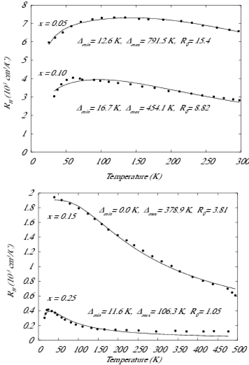
Figure 17: Fit to Hall effect datacava_hall for La_2-xSr_xCuO₄ using the expression in equation 126. For $x=0.05$, the parameters are $\Delta_{min}=12.6$ K, $\Delta_{max}=791.5$ K, and $R_{0}=15.4\times 10^{-3}$ cm³/C. For $x=0.10$, $\Delta_{min}=16.7$ K, $\Delta_{max}=454.1$ K, and $R_{0}=8.82$. For $x=0.15$, $\Delta_{min}=0.0$ K, $\Delta_{max}=387.9$ K, and $R_{0}=3.81$. For $x=0.25$, $\Delta_{min}=11.6$ K, $\Delta_{max}=106.3$ K, and $R_{0}=1.05$.

There is sufficient structure in the temperature dependence derived above to account for the various temperature behaviors of the electron-doped materials, too.kontani1

The additive contribution to the Hall resistivity arising from skew-scattering is derived in appendix B and is,

$$\rho^{skew}_{xy} = 2\left(\frac{m^{2}}{n^{2}e^{2}}\right)\left(\frac{1}{\Omega}\right)(-)\sum_{\mathbf{k^{\prime}k}}\left(-\frac{\partial f}{\partial\epsilon_{k}}\right)$$ (127)

$$\times \frac{1}{2}\left(v_{kx}v_{k^{\prime}y}-v_{ky}{v_{k^{\prime}x}}\right)w_{skew}(\mathbf{k\rightarrow k^{\prime}}).\$$

To determine if the magnitude of the chiral polaron skew-scattering is large enough to be compatible with experimental data, we computed $R_{H}c=\rho^{skew}_{xy}/B$ for La_2-xSr_xCuO₄ using the band structure in equation 62 at $x=0.10$ and estimates of various parameters.

We take $m$ to be one electron mass and $n=4x/\Omega_{cell}$ to be the number of charge carriers per volume (since each polaron adds four $x^{2}-y^{2}$ band electrons in our percolating model). The polaron g-factor is taken to be one, $g_{p}=1$. $\Delta_{max}=454.1$ K and $\Delta_{min}=16.7$ K from the fit in figure 17. Finally, we choose $\Delta^{S}_{max}=1.0$ eV and $\Delta^{D}_{max}=1.5$ eV for the energy distribution widths of the $S$ and $D_{xy}$ polaron energies.

The reason we chose $\Delta^{D}_{max}>\Delta^{S}_{max}$ is because the energy separation of the $D_{xy}$ states from the $P^{\pm}$ chiral polarons is larger than $S$ in table 2. This does not prove $\Delta^{D}_{max}>\Delta^{S}_{max}$ is always the correct choice, but it is suggestive of the expected energy splitting. Also, our values for the average skew-scattering $T$ matrix in equation 119 assume a uniform energy density $\rho^{S}$ and $\rho^{D}$ and this may not be correct. The idea here is to get a reasonable order of magnitude estimate for the size of the skew-scattering.

The final parameter to choose is the Coulomb repulsion matrix element energy $U$. $U\sim 1.0$ eV is the correct energy scale because $U=(1/\Omega_{cell})4\pi e^{2}/q_{D}^{2}$ where $q_{D}=4\pi e^{2}N(0)$ is the Debye screening length arising from the many-body response of the band electrons to a perturbing potential. $N(0)$ is the band density of states. A typical metallic density of states is one state per eV per unit cell leading to $U\sim 1.0$ eV. Since the density of charge carriers is reduced to $4x=0.40$ per unit cell, the band electrons are less effective at screening the Coulomb repulsion. This increases $U$ by a factor of $1/0.4=2.5$. We take $U=2.5$ eV.

$U$ is negative for the hole-doped cuprates because the band structure arises from fully occupied polaron states and a hole in a chiral polaron state amounts to subtracting a Coulomb matrix element. This was discussed previously following equations 96$-$101. For the electron-doped systems, $U$ is positive. Since $U^{3}$ appears in equation 119, the sign difference in the temperature dependence of the Hall effect between hole-doped and electron-doped cuprates is obtained by assuming all the other parameters discussed above do not change. We take $U=-2.5$ eV for La_2-xSr_xCuO₄.

Calculating $\rho^{skew}_{xy}$ in equation 127, we obtain $R_{H}c=5.39\times 10^{-3}\mathrm{cm}^{3}/\mathrm{C}$ at 100K or a charge density of $0.116$ carriers per unit cell with the chosen parameters. The experimental valuecava_hall for $x=0.10$ at $100$ K is approximately $4\times 10^{-3}\mathrm{cm}^{3}/\mathrm{C}$ as can be seen in figure 17. Our result is a factor of 1.35 too large.

The largest errors in our calculation come from the estimate of the Coulomb repulsion $U$, the effective $(n/m)_{eff}$, and the value of polaron g-factor, $g_{p}=1$. We used one electron mass for $m$ and chose $n$ to be $4x=0.4$ carriers per cell to obtain $(n/m)_{eff}$. This is likely an overestimate of $(n/m)_{eff}$ since the carriers must traverse a percolating swath through the crystal and the scattering rate $1/\tau$ for the ordinary conductivity is not expected to be large. Since $(n/m)_{eff}^{-2}$ and $U^{3}$ appear in $\rho_{xy}$, small changes lead to a large enhancement of the computed $\rho_{xy}$. We conclude the polaron g-factor is overestimated and may be an order of magnitude smaller, leading to $g_{p}\sim 0.1$. A reduced $g_{p}$ allows the Kondo resistivity discussed in section VII.1 to remain active in the pulsed $60$ Tesla magnetic fieldsboeb1 used to suppress superconductivity and measure the low temperature resistivity.

The analysis of this section can be done for the real polaron states $P_{x^{\prime}}$ and $P_{y^{\prime}}$ instead of the chiral states. In this case, the magnetic field creates the Van-Vleck paramagnetic states $P_{x^{\prime}}+iBP_{y^{\prime}}$ and $P_{y^{\prime}}+iBP_{x^{\prime}}$. The $B$ in the equations is a constant times the applied field. The skew-scattering contribution from a polaron where the energy of $P_{y^{\prime}}$ is greater than $P_{x^{\prime}}$ by $\Delta$ exactly cancels the contribution from a polaron where $P_{x^{\prime}}$ is greater than $P_{y^{\prime}}$ by $\Delta$. Thus, real polaron states cannot lead to skew scattering.

For a planar magnetic field, the g-factor is substantially smaller because the angular momentum of the chiral polarons is normal to the plane. Therefore, for planar magnetic fields, the Hall effect should be temperature independent, as observed.

VIII ARPES

VIII.1 Pseudogap

The undoped $d^{9}$ spins have antiferromagnetic fluctuations with wavevector $\mathbf{q}\approx(\pi,\pi)$ that couple an $x^{2}-y^{2}$ band state with momentum $\mathbf{k}$ to $\mathbf{k\pm q}$. In this section, we show that this coupling leads to a pseudogap at the Fermi energy with magnitude proportional to the square of the coupling.

At fixed temperature, the coupling is larger for low dopings because there are more undoped $d^{9}$ spins. The coupling decreases as the doping increases. This leads to a larger pseudogap for low dopings, as observed. norman1 ; loeser1 ; marshall1 ; ding1

At fixed doping, the strength of the antiferromagnetic $d^{9}$ fluctuations decreases with increasing temperature. Thus, the coupling to the $x^{2}-y^{2}$ band should decrease with increasing temperature. This leads to the closing of the pseudogap with temperature.

The momentum dependence of the pseudogap is determined by the shape of the Fermi surface. If the state with momentum $\mathbf{k\pm q}$ is close to the Fermi surface, then mixing with the $\mathbf{k}$ state leads to a reduction in the spectral function and a pseudogap. Such nesting occurs for states near $(\pm\pi,0)$ and $(0,\pm\pi)$. Along the Brillouin zone diagonals, there is no nesting. This leads to a pseudogap that is zero along the diagonal and increases as one moves toward $(\pi,0)$. The model does not guarantee zero pseudogap along the diagonal although the magnitude of the gap is expected to be small.

ARPES measures the spectral function $A(\mathbf{k},\omega)=(-1/\pi)\mathrm{Im}\ G(\mathbf{k},\omega)$. Evaluating $A(\mathbf{k},\omega)$ for $\mathbf{k}$ vectors on the Fermi surface, $\epsilon_{k}=\epsilon_{f}$, and at the Fermi energy, $\omega=\epsilon_{f}$, determines the density of states suppression at the Fermi level and its temperature dependence. The relative change in the spectral function is,

$$r(\mathbf{k},\omega,V)=\frac{A(\mathbf{k},\omega)-A_{0}(\mathbf{k},\omega)}{A_{0}(\mathbf{k},\omega)},$$ (128)

where $A_{0}(\mathbf{k},\omega)$ is the $V=0$ spectral function and $A(\mathbf{k},\omega)$ is the spectral function including the $d^{9}$ interaction $V$. The pseudogap is zero when $V=0$ at high temperature. Using equation 51,

$$r=V^{2}\cdot\frac{\mathrm{Im}\ G_{0}^{2}(\mathbf{k},\omega)\left[G_{0}(\mathbf{k+q},\omega)+G_{0}(\mathbf{k-q},\omega)\right]}{\mathrm{Im}\ G_{0}(\mathbf{k},\omega)}.$$ (129)

From equation 55,

$$G_{0}(\mathbf{k},\epsilon_{k})=\frac{1}{i\Gamma_{k}}.$$ (130)

The relative spectral function change at the Fermi level, $\omega=\epsilon_{f}$, is,

$$r = -V^{2}\left(\frac{1}{\Gamma_{k}}\right)\left[\frac{\Gamma_{k+q}}{\left(\epsilon_{f}-\epsilon_{k+q}\right)^{2}+\Gamma_{k+q}^{2}}\right.$$ (131)

$$+\left.\frac{\Gamma_{k-q}}{\left(\epsilon_{f}-\epsilon_{k-q}\right)^{2}+\Gamma_{k-q}^{2}}\right].$$

$r$ is always negative, $r<0$, and $r\rightarrow 0$ as $V\rightarrow 0$ at high temperatures. The density of states decreases at the Fermi energy leading to a temperature dependent pseudogap that closes as the temperature increases. The linewidths $\Gamma_{k}$ and $\Gamma_{k\pm q}$ are of the order $\sim 0.01$ eV due to the broadening of a $\mathbf{k}$ state arising from the non-uniform percolating path in underdoped systems. The coupling of the $d^{9}$ spins to the $x^{2}-y^{2}$ band must be less than or of the order of $J_{dd}\sim 0.1$ eV. The relative density of states change is on the order of $r\sim(V/\Gamma_{k})^{2}$. Thus, the change in the ARPES spectra arising from coupling between the undoped $d^{9}$ spins and $x^{2}-y^{2}$ is large enough to qualitatively account for the observations.

VIII.2 2212 Bi-Layer Splitting

There is an $\sim 0.1$ eV splitting between the bonding and antibonding $x^{2}-y^{2}$ bands in bilayer Bi₂Sr₂CaCu₂O_8+δ for $\mathbf{k}$ vectors near $(\pi,0)$ arising from coupling through out-of-plane orbitals. The splitting along the diagonal is very small and not experimentally resolvable. The $(\pi,0)$ splitting has been observedbilayer1 by ARPES for overdoped systems. No splitting has been observed for underdoped systems. In addition, the bilayer splitting disappears as the temperature is increased with the temperature separating the coherent (splitting) and incoherent (no splitting) regimes increasing with further overdoping.bilayer1

XAFShaskel_Sr1 ; haskel_Sr2 and first principles calculations ub3lyp_dope find the distance between an apical O and planar Cu decreases $\approx 0.2-0.3$ Å due to Sr doping in La_2-xSr_xCuO₄. Coherent hopping from one CuO₂ layer to another requires coupling of $x^{2}-y^{2}$ with an out-of-plane orbital. The $x^{2}-y^{2}$ band state is delocalized over the percolating polaron swath. Hopping onto an out-of-plane polaron orbital induces a local structural deformation. The matrix element is reduced due to the large structural change as in the small polaron problem.mahan1 The $x^{2}-y^{2}$ band electronic response to the changed potential of the doubly occupied polaron suppresses the matrix element due to the orthogonality catastrophe.mahan1

The second-order coherent bilayer hopping through an out-of-plane polaron orbital is not completely suppressed by the orthogonality catastrophe because the initial and final polaron states have the same occupation. Bilayer splitting of the $x^{2}-y^{2}$ band is induced by this coupling. The splitting is strongly temperature dependent and its magnitude decreases with increasing temperature.

In section VII.1, a similar second-order hopping leading to d-like anisotropic scattering was argued to be weakly temperature dependent. The difference between the previous intra-layer and current inter-layer process is that the matrix element for the latter is very sensitive to any out-of-plane atomic displacement leading to a strong temperature dependence.

Qualitatively, for underdoped 2212, the effective inter-layer hopping matrix element is small due to the reduced number of Cu pairs between layers that are both part of the percolating band swath. In this scenario, the bilayer splitting is small and may not have been resolved by ARPES at low temperatures.

As the doping is increased, adjacent Cu pairs between layers become available for coherent hopping and bilayer splitting becomes resolvable. This splitting decreases with increasing temperature in complete analogy to the small polaron problem. At high temperatures, the splitting disappears.

For highly overdoped materials, the splitting is large at low temperatures. As the polaron plaquettes become more crowded, any atomic distortion from hopping to or from the out-of-plane orbitals is reduced. This leads to a higher temperature before bilayer splitting becomes too small to be resolvable by ARPES.

IX NMR

A potential problem with our chiral plaquette polaron theory of cuprate superconductivity involves the NMR experiments by Takigawa et altakigawa1 on underdoped YBa₂Cu₃O_6.63 that shows the same temperature dependent Knight shift for both the planar Cu and O. The most reasonable conclusion from this experiment is that only one electronic component is involved in the cuprate NMR. Similar conclusions were reached for La_2-xSr_xCuO₄.johnston1 ; nakano1 ; walstedt2 This would appear to contradict our assertion of an out-of-plane polaron because one would expect the polaron to have different hyperfine couplings to the planar Cu and O atoms than the $x^{2}-y^{2}$ band, leading to a total Knight Shift temperature dependence (sum of $x^{2}-y^{2}$ band plus polaron) that is different for Cu and O.

On the other hand, small-tip angle spin-echo double resonance (SEDOR) measurementspennington1 find the electron mediated nuclear-nuclear couplings between neighboring Cu-O and Cu-Cu are incompatible with one-component cuprate theories. In addition, the high-temperature Y spin relaxation and Knight Shiftsnandor1 are incompatible with one-component cuprate theories. Indeed, recent phenomenological fitsuldry1 imply there are two contributions to the Redfield correlation time.

Clearly the effect of the out-of-plane orbitals in our model cannot be ignored in interpreting the NMR data. In our model, the polarons lead to a weakly temperature dependent Knight shift of the form in equation 125 for the magnetic susceptibility due to polarons and shown in figure 17 for the temperature dependence of the Hall effect. The polaron hyperfine coupling to the planar Cu and O sites is weaker than the $x^{2}-y^{2}$ band because the hole character is primarily in the out-of-plane O $p_{z}$ orbital. This weak temperature dependence is seen in fully doped YBa₂Cu₃O₇ because the $x^{2}-y^{2}$ band electrons Knight shift contribution is constant with temperature.nandor1 For underdoped samples, the temperature dependence of the polaron shift is masked by the larger temperature dependence of the Knight shift from the $x^{2}-y^{2}$ band electrons. The latter shift arises from the decrease in the density of states of the $x^{2}-y^{2}$ band due to the coupling with the undoped Cu $d^{9}$ spins as shown in equation 131 for the ARPES pseudogap. We intend to develop the methodology to estimate the size of these effects and their detailed temperature dependence in order to compare the results with experimental data. However, at the present time the NMR must be considered a possible Achilles Heel for our chiral plaquette polaron theory of cuprate superconductivity.

X Conclusions

Ab-initio quantum mechanical calculations find localized holes in out-of-plane orbitals in contrast to the t-J model. Based on the results of calculations with explicity doped Sr in La_2-xSr_xCuO₄, we postulated that chiral plaquette polarons are created by doping and that a delocalized $x^{2}-y^{2}$/$p_{\sigma}$ band is formed when the plaquette polarons percolate through the crystal.

The D-wave superconductivity, temperature dependent Hall effect, neutron $\omega/T$ scaling, neutron incommensurability, resistivity, the doping value for the insulator-metal phase transition, optical absorption, low-temperature $\log(T)$ resistivity, ARPES pseudogap, and the evolution of bi-layer splitting in Bi-2212 are explained by chiral plaquette polarons.

We have not shown ab-initio that chiral plaquette polarons are formed with doping. For La_2-xSr_xCuO₄, ab-initio evidence for holes in out-of-plane orbitals has been demonstrated. Out-of-plane hole orbitals are plausible for cuprates where the doping arises from interstitial O atoms. YBa₂Cu₃O₇, where the Cu$-$O chain is completely full, is most intriguing. We believe there are local structural deformations of the apical O atoms favoring localized out-of-plane orbitals.

Detailed calculations of the spectral function for the $x^{2}-y^{2}$ band measured in ARPES are necessary in order to study the evolution of the background and linewidth as a function of doping and temperature. For underdoped systems, the percolating path is not uniform through the crystal and leads to broadening of the $\mathbf{k}$ state spectral function. Mixing with the A₁ orbitals of the polarons increases the broadening near $(\pi,0)$.

A calculation using the Coherent Potential Approximation (CPA)cpa1 ; cpa2 may be the way to obtain quantitative estimates of the ARPES. CPA calculations would lead to an accurate determination of the magnitude of the resistivity and would allow us to determine the correct value of $(n/m)_{eff}$ to use in the results for the magnitude of the skew-scattering contribution to the Hall effect.

Since neutron spin scattering couples to the electron spin and transport couples to its charge, we regard our results to be strong evidence for the existence of chiral plaquette polarons.

Appendix A Perturbed Band Energy

In this appendix, we derive the expressions used in section V.3 to compute the contribution of the $x^{2}-y^{2}$ band energy for different incommensurate neutron q-vectors.

Using equations 53, 55, and V.3,

$$n(\mathbf{k},\epsilon)=n_{0}(\mathbf{k},\epsilon)+V^{2}\int_{-\infty}^{\epsilon}d\omega\ P(\mathbf{k},\omega),$$ (132)

where we have defined,

$$P(\mathbf{k},\omega)=R(\mathbf{k},\mathbf{k+q},\omega)+R(\mathbf{k},\mathbf{k-q},\omega).$$ (133)

The total number of electrons is $n_{tot}=\sum_{\mathbf{k}}n(\mathbf{k},\epsilon_{f}+\delta\epsilon_{f})$. From equation 132,

$$n_{tot}=\sum_{\mathbf{k}}n_{0}(\mathbf{k},\epsilon_{f}+\delta\epsilon_{f})+V^{2}\int_{-\infty}^{\epsilon_{f}+\delta\epsilon_{f}}d\omega\sum_{\mathbf{k}}P(\mathbf{k},\omega).$$ (134)

The first term on the right-hand side can be expanded in a power series in $\delta\epsilon_{f}$,

$$\sum_{\mathbf{k}}n_{0}(\mathbf{k},\epsilon_{f})+\delta\epsilon_{f}\frac{\partial}{\partial\epsilon}\left[\sum_{\mathbf{k}}n_{0}(\mathbf{k},\epsilon_{f})\right]+O(\delta\epsilon_{f}^{2})$$

$$=n_{tot}+\delta\epsilon_{f}N_{0}(\epsilon_{f})+O(\delta\epsilon_{f}^{2}),$$ (135)

where we have used equations 54 and 57. $N_{0}(\epsilon_{f})$ is the unperturbed density of states per spin. The second term in equation 134 becomes,

$$V^{2}\int_{-\infty}^{\epsilon_{f}}d\omega\sum_{\mathbf{k}}P(\mathbf{k},\omega)+O(V^{2}\delta\epsilon_{f}).$$ (136)

Since $\delta\epsilon_{f}\sim O(V^{2})$, the second term is of order $\delta\epsilon_{f}^{2}\sim O(V^{4})$ and can be neglected to lowest order. Substituting into 134 leads to,

$$\delta\epsilon_{f}N_{0}(\epsilon_{f})+V^{2}\int_{-\infty}^{\epsilon_{f}}d\omega\sum_{\mathbf{k}}P(\mathbf{k},\omega)=0.$$ (137)

From equation 133, 137 is identical equation V.3.

Substituting 132 into equation 58 for the total energy, using equation 54, and keeping terms up to $O(V^{2})$,

$$E_{tot}(\mathbf{q},V) = E_{G}+\epsilon_{f}\cdot\delta\epsilon_{f}N_{0}(\epsilon_{f})$$ (138)

$$+V^{2}\int_{-\infty}^{\epsilon_{f}}d\omega\ \omega\sum_{\mathbf{k}}P(\mathbf{k},\omega).$$

The second term proportional to $\delta\epsilon_{f}$ can be eliminated by using equation 137 leading to,

$$E_{tot}(\mathbf{q},V)=E_{G}+V^{2}\int_{-\infty}^{\epsilon_{f}}d\omega(\omega-\epsilon_{f})\sum_{\mathbf{k}}P(\mathbf{k},\omega).$$ (139)

$E_{G}$ is the unperturbed $(V=0)$ ground state energy. Using 133, this is the result shown in equation V.3.

To compute the change in energy due to incommensurability, we need to evaluate integrals of the form,

$$I(E,E^{\prime},\epsilon_{f})\equiv\int_{-\infty}^{\epsilon_{f}}\frac{d\omega}{\left(\omega-E\right)^{2}\left(\omega-E^{\prime}\right)},$$ (140)

$$J(E,E^{\prime},\epsilon_{f})\equiv\int_{-\infty}^{\epsilon_{f}}d\omega\frac{\left(\omega-\epsilon_{f}\right)}{\left(\omega-E\right)^{2}\left(\omega-E^{\prime}\right)},$$ (141)

where

$$E=\epsilon-i\Gamma,\ E^{\prime}=\epsilon^{\prime}-i\Gamma^{\prime}\ \ \mathrm{and}\ \Gamma,\ \Gamma^{\prime}>0.$$ (142)

From equation 61,

$$\int_{-\infty}^{\epsilon_{f}}R(\mathbf{k},\mathbf{p},\omega)d\omega=\ \ \ \ \ \ \ \ \ \ \$$

$$\left(-\frac{1}{\pi}\right)\mathrm{Im}\ I(\epsilon_{k}-i\Gamma_{k},\epsilon_{p}-i\Gamma_{p},\epsilon_{f}).$$ (143)

The imaginary part of $J(E,E^{\prime},\epsilon_{f})$ appears in 139.

The integrand of 140 can be expanded in partial fractions,

$$\frac{1}{\left(\omega-E\right)^{2}\left(\omega-E^{\prime}\right)} = \delta E^{-2}\left(\frac{1}{\omega-E^{\prime}}-\frac{1}{\omega-E}\right)$$ (144)

$$- \delta E^{-1}\frac{1}{\left(\omega-E\right)^{2}},$$

where $\delta E=E^{\prime}-E$. The second term on the right-hand side can be integrated,

$$\int_{-\infty}^{\epsilon_{f}}d\omega\frac{(-)}{\left(\omega-E\right)^{2}}=\frac{1}{\epsilon_{f}-E}.$$ (145)

Each individual integral in the first term is infinite. The integral is performed by substituting $-\Lambda$ for $-\infty$ and taking the limit $\Lambda\rightarrow+\infty$.

$$\mathrm{Re}\int_{-\Lambda}^{\epsilon_{f}}d\omega\left[\frac{1}{\omega-E^{\prime}}-\frac{1}{\omega-E}\right]=\ \ \ \ \ \ \$$

$$\int_{-\Lambda}^{\epsilon_{f}}d\omega\left[\frac{\left(\omega-\epsilon^{\prime}\right)}{\left(\omega-\epsilon^{\prime}\right)^{2}+\Gamma^{\prime 2}}-\frac{\left(\omega-\epsilon\right)}{\left(\omega-\epsilon\right)^{2}+\Gamma^{2}}\right],$$ (146)

$$\mathrm{Im}\int_{-\Lambda}^{\epsilon_{f}}d\omega\left[\frac{1}{\omega-E^{\prime}}-\frac{1}{\omega-E}\right]=\ \ \ \ \ \ \$$

$$\int_{-\Lambda}^{\epsilon_{f}}d\omega\left[\frac{\Gamma}{\left(\omega-\epsilon\right)^{2}+\Gamma^{2}}-\frac{\Gamma^{\prime}}{\left(\omega-\epsilon^{\prime}\right)^{2}+\Gamma^{\prime 2}}\right].$$ (147)

The real part can be solved,

$$\int_{(-\Lambda-\epsilon^{\prime})/\Gamma^{\prime}}^{(\epsilon_{f}-\epsilon^{\prime})/\Gamma^{\prime}}\frac{xdx}{x^{2}+1}-\int_{(-\Lambda-\epsilon)/\Gamma}^{(\epsilon_{f}-\epsilon)/\Gamma}\frac{xdx}{x^{2}+1}=\ \ \ \$$

$$\frac{1}{2}\ln\left[\frac{\left(\epsilon_{f}-\epsilon^{\prime}\right)^{2}/\Gamma^{\prime 2}+1}{\left(\epsilon_{f}-\epsilon\right)^{2}/\Gamma^{2}+1}\right]\ \ \ \ \ \ \ \ \ \$$

$$+\ \ \frac{1}{2}\ln\left[\frac{\left(-\Lambda-\epsilon\right)^{2}/\Gamma^{2}+1}{\left(-\Lambda-\epsilon^{\prime}\right)^{2}/\Gamma^{\prime 2}+1}\right].\ \ \ \$$ (148)

Taking the limit $\Lambda\rightarrow+\infty$, the real part becomes,

$$\mathrm{Re}\int_{-\infty}^{\epsilon_{f}}d\omega\left[\frac{1}{\omega-E^{\prime}}-\frac{1}{\omega-E}\right]=\frac{1}{2}\ln\left[\frac{\Gamma^{\prime 2}\left(x^{\prime 2}+1\right)}{\Gamma^{2}\left(x^{2}+1\right)}\right].$$ (150)

The imaginary part integrates to,

$$\mathrm{Im}\int_{-\infty}^{\epsilon_{f}}d\omega\left[\frac{1}{\omega-E^{\prime}}-\frac{1}{\omega-E}\right] = \tan^{-1}x$$ (151)

$$- \tan^{-1}x^{\prime},$$

where $x=(\epsilon_{f}-\epsilon)/\Gamma$ and $x^{\prime}=(\epsilon_{f}-\epsilon^{\prime})/\Gamma^{\prime}$. Substituting into equation 140,

$$I(E,E^{\prime},\epsilon_{f}) = \delta E^{-2}\left\{\frac{1}{2}\ln\left[\frac{\Gamma^{\prime 2}\left(x^{\prime 2}+1\right)}{\Gamma^{2}\left(x^{2}+1\right)}\right]\right.$$ (152)

$$+ \left.i\left(\tan^{-1}x-\tan^{-1}x^{\prime}\right)\right\}$$

$$+ \delta E^{-1}\cdot\frac{1}{\epsilon_{f}-E},$$

where $E$ and $E^{\prime}$ are defined in equation 142 and $\delta E=E^{\prime}-E$.

Writing $\omega-\epsilon_{f}=(\omega-E^{\prime})+(E^{\prime}-\epsilon_{f})$ in equation 141 for $J(E,E^{\prime},\epsilon_{f})$,

$$J(E,E^{\prime},\epsilon_{f})=\left(E^{\prime}-\epsilon_{f}\right)I(E,E^{\prime},\epsilon_{f})-\frac{1}{\left(\epsilon_{f}-E\right)},$$ (153)

leading to,

$$J(E,E^{\prime},\epsilon_{f}) = \frac{\left(E^{\prime}-\epsilon_{f}\right)}{\left(E^{\prime}-E\right)^{2}}\left\{\frac{1}{2}\ln\left[\frac{\Gamma^{\prime 2}\left(x^{\prime 2}+1\right)}{\Gamma^{2}\left(x^{2}+1\right)}\right]\right.$$ (154)

$$+ \left.i\left(\tan^{-1}x-\tan^{-1}x^{\prime}\right)\right\}$$

$$+ \frac{1}{E-E^{\prime}}.$$

Appendix B Hall Effect

In this appendix, we derive equations 110-113 and 127 in section VII.2. Equation 107 is

$$V^{(2)(\pm)}_{\mathbf{k^{\prime}k}}=\sum_{\mathbf{p}}\frac{\langle\mathbf{k^{\prime}}P^{\pm}|H_{U}|\mathbf{p}I\rangle\langle\mathbf{p}I|H_{U}|\mathbf{k}P^{\pm}\rangle}{\epsilon_{k}-\epsilon_{p}-\left(E_{I}-E^{\pm}\right)+i\delta}.$$ (155)

Expanding for $I=S$ using equation 96,

$$V^{(2)(\pm)}_{\mathbf{k^{\prime}k}}(S)=\left(\frac{U}{2N}\right)^{2}\sum_{\mathbf{p}}\frac{\left[\sin\left(k^{\prime}-p\right)_{x^{\prime}}\mp i\sin\left(k^{\prime}-p\right)_{y^{\prime}}\right]\left[\sin\left(k-p\right)_{x^{\prime}}\mp i\sin\left(k-p\right)_{y^{\prime}}\right]^{\ast}}{\epsilon_{k}-\epsilon_{p}-\left(E_{S}-E^{\pm}\right)+i\delta}.$$ (156)

Expanding the numerator inside the summation into products $\sin k^{\prime}_{x^{\prime}}\cos p_{x^{\prime}}$ etc,

$$\mathrm{Num} = \left[\left(\sin k^{\prime}_{x^{\prime}}\cos p_{x^{\prime}}-\cos k^{\prime}_{x^{\prime}}\sin p_{x^{\prime}}\right)\right.\mp\left.i\left(\sin k^{\prime}_{y^{\prime}}\cos p_{y^{\prime}}-\cos k^{\prime}_{y^{\prime}}\sin p_{y^{\prime}}\right)\right]$$ (157)

$$\times \left[\left(\sin k_{x^{\prime}}\cos p_{x^{\prime}}-\cos k_{x^{\prime}}\sin p_{x^{\prime}}\right)\right.\mp\left.i\left(\sin k_{y^{\prime}}\cos p_{y^{\prime}}-\cos k_{y^{\prime}}\sin p_{y^{\prime}}\right)\right]^{\ast}.$$

This can be further expanded into terms with products of the form $\cos^{2}p_{x^{\prime}}$, $\cos p_{x^{\prime}}\cos p_{y^{\prime}}$, $\cos p_{x^{\prime}}\sin p_{y^{\prime}}$, etc.

The denominator in equation 156 only depends on $\mathbf{p}$ through the energy $\epsilon_{p}$ and has $D_{4h}$ crystal symmetry. Thus, for each $\mathbf{p}$, the sum includes terms with $p_{x^{\prime}}\rightarrow-p_{x^{\prime}}$ and $p_{y^{\prime}}\rightarrow-p_{y^{\prime}}$. The only non-zero terms in the numerator have products $\cos^{2}p_{x^{\prime}}$, $\cos^{2}p_{y^{\prime}}$, $\cos p_{x^{\prime}}\cos p_{y^{\prime}}$, $\sin^{2}p_{x^{\prime}}$, and $\sin^{2}p_{y^{\prime}}$.

The real part of the numerator is,

$$\mathrm{Re(Num)} = \left[\left(\sin k^{\prime}_{x^{\prime}}\sin k_{x^{\prime}}\cos^{2}p_{x^{\prime}}\right.\right.$$ (158)

$$+ \left.\cos k^{\prime}_{x^{\prime}}\cos k_{x^{\prime}}\sin^{2}p_{x^{\prime}}\right)$$

$$+ \left(\sin k^{\prime}_{y^{\prime}}\sin k_{y^{\prime}}\cos^{2}p_{y^{\prime}}\right.$$

$$+ \left.\left.\cos k^{\prime}_{y^{\prime}}\cos k_{y^{\prime}}\sin^{2}p_{y^{\prime}}\right)\right].$$

Using $\cos^{2}p_{x^{\prime}}=1/2(1+\cos 2p_{x^{\prime}})$ and $\sin^{2}p_{x^{\prime}}=1/2(1-\cos 2p_{x^{\prime}})$ with similar equations for $p_{y^{\prime}}$,

$$\mathrm{Re(Num)}=\frac{1}{2}\left[\cos(k^{\prime}-k)_{x^{\prime}}+\cos(k^{\prime}-k)_{y^{\prime}}\right]$$

$$-\frac{1}{2}\left[\cos(k^{\prime}+k)_{x^{\prime}}+\cos(k^{\prime}+k)_{y^{\prime}}\right]\cos 2p_{x^{\prime}},$$ (159)

where we have used $\cos 2p_{y^{\prime}}=\cos 2p_{x^{\prime}}$ due to symmetry in the summation. The definitions of the primed coordinates in equations 102 and 103 lead to,

$$\mathrm{Re(Num)}=\cos\frac{1}{2}\left(k^{\prime}_{x}-k_{x}\right)\cos\frac{1}{2}\left(k^{\prime}_{y}-k_{y}\right)$$

$$-\cos 2p_{x^{\prime}}\cos\frac{1}{2}\left(k^{\prime}_{x}+k_{x}\right)\cos\frac{1}{2}\left(k^{\prime}_{y}+k_{y}\right).$$ (160)

A similar expansion for the imaginary part leads to,

$$\mathrm{Im(Num)} = \left(\mp\right)\left(\sin k_{x^{\prime}}\sin k^{\prime}_{y^{\prime}}\right.$$ (161)

$$- \left.\sin k_{y^{\prime}}\sin k^{\prime}_{x^{\prime}}\right)\cos p_{x^{\prime}}\cos p_{y^{\prime}}$$

$$= A_{\mathbf{k^{\prime}k}}\cos p_{x^{\prime}}\cos p_{y^{\prime}},$$

with $A_{\mathbf{k^{\prime}k}}$ defined in equation 112. Collecting the real and imaginary terms,

$$V^{(2)(\pm)}_{\mathbf{k^{\prime}k}}(S) = \left(\frac{U}{4N}\right)^{2}$$ (162)

$$\times \left\{\tilde{F}_{0}(\omega_{0})\cos\frac{1}{2}\left(k^{\prime}_{x}-k_{x}\right)\cos\frac{1}{2}\left(k^{\prime}_{y}-k_{y}\right)\right.$$

$$- \tilde{F}_{2}(\omega_{0})\cos\frac{1}{2}\left(k^{\prime}_{x}+k_{x}\right)\cos\frac{1}{2}\left(k^{\prime}_{y}+k_{y}\right)$$

$$\mp \left.i\tilde{F}_{1}(\omega_{0})A_{\mathbf{k^{\prime}k}}\right\},$$

where $\omega_{0}=\epsilon_{k}-(E_{S}-E^{\pm})$ and the $\tilde{F}$ functions are defined as,

$$\tilde{F}_{0}(\omega)=\left(\frac{1}{N}\right)\sum_{\mathbf{p}}\frac{1}{\omega-\epsilon_{p}+i\delta},$$ (163)

$$\tilde{F}_{1}(\omega)=\left(\frac{1}{N}\right)\sum_{\mathbf{p}}\frac{\cos p_{x^{\prime}}\cos p_{y^{\prime}}}{\omega-\epsilon_{p}+i\delta},$$ (164)

$$\tilde{F}_{2}(\omega)=\left(\frac{1}{N}\right)\sum_{\mathbf{p}}\frac{\cos 2p_{x^{\prime}}}{\omega-\epsilon_{p}+i\delta}.$$ (165)

Expanding the cosines in 164 and 165,

$$\cos p_{x^{\prime}}\cos p_{y^{\prime}}=\frac{1}{2}\left(\cos p_{x}+\cos p_{y}\right),$$ (166)

$$\cos 2p_{x^{\prime}}=\cos(p_{x}+p_{y}) = \cos p_{x}\cos p_{y}$$ (167)

$$- \sin p_{x}\sin p_{y}.$$

The second term in equation 167 averages to zero when summed in $\tilde{F}_{2}$. $\tilde{F}_{1}$ and $\tilde{F}_{2}$ become

$$\tilde{F}_{1}(\omega)=\left(\frac{1}{N}\right)\sum_{\mathbf{p}}\frac{\frac{1}{2}\left(\cos p_{x}+\cos p_{y}\right)}{\omega-\epsilon_{p}+i\delta},$$ (168)

$$\tilde{F}_{2}(\omega)=\left(\frac{1}{N}\right)\sum_{\mathbf{p}}\frac{\cos p_{x}\cos p_{y}}{\omega-\epsilon_{p}+i\delta}.$$ (169)

The equation for $V^{(2)(\pm)}_{\mathbf{k^{\prime}k}}(D)$ is the same as equation 162 with $E_{S}\rightarrow E_{D}$ and $\mp(i)\rightarrow\pm(i)$.

From equation 109, the real part of $V^{(2)(\pm)}_{\mathbf{k^{\prime}k}}(S)$ is necessary for the lowest order skew-scattering. In addition, only terms antisymmetric under interchange of $\mathbf{k^{\prime}}$ and $\mathbf{k}$ contribute to $\rho^{skew}_{xy}$. The last term in equation 162 is antisymmetric and only the imaginary part of $\tilde{F}_{1}$ contributes to the skew-scattering.

Defining $F_{1}(\omega)=(-1/\pi)\mathrm{Im}\tilde{F}_{1}(\omega)$,

$$F_{1}(\omega)=\left(\frac{1}{N}\right)\sum_{\mathbf{p}}\frac{1}{2}\left(\cos p_{x}+\cos p_{y}\right)\delta(\omega-\epsilon_{p}),$$ (170)

leads to equations 110 and 111.

Equation 127 for the skew-scattering is obtained by solving the linearized Boltzmann transport equation for skew-scattering,varma1 ; skew_boltz1 ; skew_boltz2

$$\left(\frac{\partial f_{k}}{\partial t}\right)_{field}+\left(\frac{\partial f_{k}}{\partial t}\right)_{scatt}=0,$$ (171)

$$\left(\frac{\partial f_{k}}{\partial t}\right)_{field} = \left(\frac{\partial f_{0}}{\partial\epsilon_{k}}\right)(-e)\left(\mathbf{v_{k}\cdot E}\right)$$ (172)

$$+ \left(\frac{e}{\hbar c}\right)\frac{\partial g_{k}}{\partial\mathbf{k}}\cdot\left(\mathbf{v_{k}\wedge B}\right),$$

$$\left(\frac{\partial f_{k}}{\partial t}\right)_{scatt} = -\frac{g_{k}}{\tau_{k}}+\sum_{k^{\prime}}\left[-w_{skew}\left(k\rightarrow k^{\prime}\right)g_{k}\right.$$ (173)

$$+ \left.w_{skew}\left(k^{\prime}\rightarrow k\right)g_{k^{\prime}}\right],$$

where $e>0$ and $f_{k}=f_{0}+g_{k}$ with $f_{0}$ the Fermi-Dirac function at energy $\epsilon_{k}$. $1/\tau_{k}$ is the ordinary scattering rate. This is given by equation 89 in our model. From equations 119$-$121, $\sum_{k^{\prime}}w_{skew}(k\rightarrow k^{\prime})=0$ making the second term on the right hand side of equation 173 vanish.

Substituting,

$$g_{k}=\left(-\frac{\partial f_{0}}{\partial\epsilon_{k}}\right)\Phi_{k},$$ (174)

the transport equation becomes,

$$-e\left(\mathbf{v_{k}\cdot E}\right)+\left(\frac{e}{\hbar c}\right)\frac{\partial\Phi_{k}}{\partial\mathbf{k}}\cdot\left(\mathbf{v_{k}\wedge B}\right)$$

$$-\frac{\Phi_{k}}{\tau_{k}}-\sum_{k^{\prime}}w_{skew}(k\rightarrow k^{\prime})\Phi_{k^{\prime}}=0.$$ (175)

$\Phi_{k}$ can be expanded in the series,

$$\Phi_{k}=\Phi^{(0)}_{k}+\Phi^{(1)(ord)}_{k}+\Phi^{(1)(skew)}_{k}+\ldots,$$ (176)

where $\Phi^{(0)}\sim O(E)$ and $\Phi^{(1)}\sim O(EB)$. $\Phi^{(1)(ord)}_{k}$ is the ordinary band contribution to the Hall effect. We do not write down the expression for this term. The second $O(EB)$ term, $\Phi^{(1)(skew)}_{k}$, is the additional contribution arising from the skew-scattering term, $w_{skew}$. Substituting 176 into B leads to,

$$\Phi^{(0)}=-e\left(\tau_{k}\mathbf{v_{k}\cdot E}\right),$$ (177)

$$\Phi^{(1)(skew)}=\sum_{k^{\prime}}\tau_{k}\tau_{k^{\prime}}e\left(\mathbf{v_{k}\cdot E}\right)w_{skew}(k\rightarrow k^{\prime}).$$ (178)

The current density per spin is,

$$\mathbf{J}=\left(\frac{1}{\Omega}\right)\sum_{k}(-e)g_{k}\mathbf{v_{k}},$$ (179)

where $\Omega$ is the total volume. The $O(EB)$ contribution to the conductivity per spin $\sigma_{yx}^{skew}$ from skew-scattering satisfies $J_{y}^{(1)(skew)}=\sigma_{yx}^{skew}E_{x}$,

$$\sigma_{yx}^{skew} = (-e^{2})\left(\frac{1}{\Omega}\right)\sum_{kk^{\prime}}\left(-\frac{\partial f_{0}}{\partial\epsilon_{k}}\right)\tau_{k}\tau_{k^{\prime}}$$ (180)

$$\times v_{ky}v_{k^{\prime}x}w_{skew}(k\rightarrow k^{\prime}).$$

Using $\sigma_{yx}=-\sigma_{xy}$ from crystal symmetry and $\rho_{xy}=\sigma_{xy}/\sigma^{2}$ for the Hall resistivity,

$$\rho_{xy}^{skew}\sigma^{2} = (2e^{2})\left(\frac{1}{\Omega}\right)\sum_{kk^{\prime}}\left(-\frac{\partial f_{0}}{\partial\epsilon_{k}}\right)\tau_{k}\tau_{k^{\prime}}$$ (181)

$$\times v_{ky}v_{k^{\prime}x}w_{skew}(k\rightarrow k^{\prime}),$$

with the additional factor of $2$ on the right hand side to include spin. The conductivity $\sigma$ is,

$$\sigma=e^{2}\tau\left(\frac{n}{m}\right)_{eff},$$ (182)

where $(n/m)_{eff}$ is the effective $n/m$ and we have taken $\tau_{k}$ to be independent of k and equal to $\tau$. Since $\rho_{yx}=-\rho_{xy}$ by symmetry, we symmetrize the expression for $\rho_{xy}$ by setting $\rho_{xy}=(1/2)(\rho_{xy}-\rho_{yx})$, leading to equation 127.

References

• (1) P. W. Anderson, Science 235, 1196 (1987).
• (2) V. J. Emery, Phys. Rev. Lett. 58, 2794 (1987).
• (3) J. G. Bednorz and K. A. Muller, Z. Phys. B 64, 189 (1987).
• (4) B. I. Shraiman and E. D. Siggia, Phys. Rev. B 42, 2485 (1990).
• (5) B. I. Shraiman and E. D. Siggia, Phys. Rev. Lett. 61, 467 (1988).
• (6) B. I. Shraiman and E. D. Siggia, Phys. Rev. Lett. 62, 1564 (1989).
• (7) X. G. Wen, F. Wilczek, and A. Zee, Phys. Rev. B 39, 11413 (1988).
• (8) R. J. Gooding, Phys. Rev. Lett. 66, 2266, (1991).
• (9) J. K. Perry, J. Tahir-Kheli, and W. A. Goddard III, Phys. Rev. B 65, 144501 (2002).
• (10) M. A. Kastner, R. J. Birgeneau, G. Shirane, and Y. Endoh, Rev. Mod. Phys. 70, 897 (1998).
• (11) H. Takagi, R. J. Cava, M. Marezio, B. Batlogg, J. J. Krajewski, W. F. Peck Jr., P. Bordet, and D. E. Cox, Phys. Rev. Lett. 68, 3777 (1992).
• (12) R. Liang, D. A. Bonn, W. N. Hardy, J. C. Wynn, K. A. Moler, L. Lu, S. Larochelle, L. Zhou, M. Greven, L. Lurio, and S. G. J. Mochrie, Physica C 383, 1 (2002).
• (13) R. J. Gooding, N. M. Salem, R. J. Birgeneau, and F. C. Chou, Phys. Rev. B 55, 6360 (1996).
• (14) P. Gawiec and D. R. Grempel, Phys. Rev. B 44, 2613 (1991).
• (15) H. S. Yoshizawa, S. Mitsuda, H. Kitazawa, and K. Katsumata, J. Phys. Soc. Jpn. 57, 3686 (1988).
• (16) S.-W. Cheong, G. Aeppli, T. E. Mason, H. Mook, S. M. Hayden, P. C. Canfield, Z. Fisk, K. N. Clausen, and J. L. Martinez, Phys. Rev. Lett. 67, 1791 (1991).
• (17) R. J. Birgeneau, Y. Endoh, K. Kakurai, Y. Hidaka, T. Murakami, M. A. Kastner, T. R. Thurston, G. Shirane, and K. Yamada, Phys. Rev. B 39, 2868 (1989).
• (18) B. Keimer, R. J. Birgeneau, A. Cassanho, Y. Endoh, R. W. Erwin, M. A. Kastner, and G. Shirane, Phys. Rev. Lett. 67, 1930 (1991).
• (19) S. M. Hayden, G. Aeppli, R. Osborn, A. D. Taylor, T. G. Perring, S.-W. Cheong, and Z. Fisk, Phys. Rev. Lett. 67, 3622 (1991).
• (20) M. Matsuda, R. J. Birgeneau, Y. Endoh, Y. Hidaka, M. A. Kastner, K. Nakajima, G. Shirane, T. R. Thurston, and K. Yamada, J. Phys. Soc. Japan 62, 1702 (1993).
• (21) K. Kakurai, S. Shamoto, T. Kiyokura, M. Sato, J. M. Tranquada, and G. Shirane, Phys. Rev. B 48, 3485 (1993).
• (22) R. J. Birgeneau, R. W. Erwin, P. M. Gehring, M. A. Kastner, B. Keimer, M. Sato, S. Shamoto, G. Shirane, and J. Tranquada, Z. Phys. B 87, 15 (1992).
• (23) B. J. Sternlieb, G. Shirane, J. M. Tranquada, M. Sato, and S. Shamoto, Phys. Rev. B 47, 5320 (1993).
• (24) G. Aeppli, T. E. Mason, S. M. Hayden, H. A. Mook, and J. Kulda, Science 278, 1432 (1997)
• (25) A. Fert and P. M. Levy, Phys. Rev. B 36, 1907 (1987).
• (26) A. Fert, J. Phys. F 3, 2126 (1973).
• (27) A. Fert and O. Jaoul, Phys. Rev. Lett. 28, 303 (1972).
• (28) P. Coleman, P. W. Anderson, and T. V. Ramakrishnan, Phys. Rev. Lett. 55, 414 (1985).
• (29) H. Y. Hwang, B. Batlogg, H. Takagi, H. L. Kao, J. Kwo, R. J. Cava, J. J. Krajewski, and W. F. Peck, Jr., Phys. Rev. Lett. 72, 2636 (1994).
• (30) H. Kontani, K. Kanki, and K. Ueda, Phys. Rev. B 59, 14723 (1999).
• (31) M. R. Norman, H. Ding, M. Randeria, J. C. Campuzano, T. Yokoya, T. Takeuchi, T. Takahashi, T. Mochiku, K. Kadowaki, P. Guptasarma, and D. G. Hinks, Nature 392, 157 (1998).
• (32) A. G. Loeser, Z.-X. Shen, D. S. Dessau, D. S. Marshall, C. H. Park, P. Fournier, and A. Kapitulnik, Science 273, 325 (1996).
• (33) D. S. Marshall, D. S. Dessau, A. G. Loeser, C. H. Park, A. Y. Matsuura, J. N. Eckstein, I. Bozovic, P. Fournier, A. Kapitulnik, W. E. Spicer, and Z.-X. Shen, Phys. Rev. Lett. 76, 4841 (1996).
• (34) H. Ding, T. Yokoya, J. C. Campuzano, T. Takahashi, M. Randeria, M. R. Norman, R. Mochiku, K. Kadowaki, and J. Giapintzakis, Nature 382, 51 (1996).
• (35) N. B. Brookes, G. Ghiringhelli, O. Tjernberg, L. H. Tjeng, T. Mizokawa, T. W. Li, and A. A. Menovsky, Phys. Rev. Lett. 87, 237003 (2001).
• (36) L. H. Tjeng, B. Sinkovic, N. B. Brookes, J. B. Goedkoop, R. Hesper, E. Pellegrin, F. M. F. de Groot, S. Altieri, S. L. Hulbert, E. Shekel, and G. A. Sawatzky, Phys. Rev. Lett. 78, 1126 (1996).
• (37) C. T. Chen, L. H. Tjeng, J. Kwo, H. L. Kao, P. Rudolf, F. Sette, and R. M. Fleming, Phys. Rev. Lett. 68, 2543 (1992).
• (38) M. Takigawa, A. P. Reyes, P. C. Hammel, J. D. Thompson, R. H. Heffner, Z. Fisk, and K. C. Ott, Phys. Rev. B 43, 247 (1991).
• (39) A. D. Becke, J. Chem. Phys. 98, 1372 (1993).
• (40) A. D. Becke, J. Chem. Phys. 98, 5648 (1993).
• (41) A. D. Becke, Phys. Rev. A 38, 3098 (1988).
• (42) C. Lee, W. Yang, and R. G. Parr, Phys. Rev. B 37, 785 (1988).
• (43) S. H. Vosko, L. Wilk, and M. Nusair, Can. J. Phys. 58, 1200 (1980).
• (44) A. Ricca and C. W. Bauschlicher, J. Phys. Chem. 98, 12899 (1994).
• (45) T. V. Russo, R. L. Martin, and P. J. Hay, J. Chem. Phys. 102, 8023 (1995).
• (46) L. Rodriguez-Santiago, M. Sodupe, and V. Branchadell, J. Chem. Phys. 105, 9966 (1996).
• (47) P. E. M. Siegbahn and R. H. Crabtree, J. Am. Chem. Soc. 119, 3103 (1997).
• (48) J. K. Perry, J. Tahir-Kheli, and W. A. Goddard III, Phys. Rev. B 63, 144510 (2001).
• (49) J. M. Ginder, M. G. Roe, Y. Song, R. P. McCall, J. R. Gaines, E. Ehrenfreund, and A. J. Epstein, Phys. Rev. B 37, 7506 (1988).
• (50) J. Yu, A. J. Freeman, and J. H. Xu, Phys. Rev. Lett. 58, 1035 (1987).
• (51) L. F. Mattheiss, Phys. Rev. Lett. 58, 1028 (1987).
• (52) W. E. Pickett, Rev. Mod. Phys. 61, 433 (1989).
• (53) A. Svane, Phys. Rev. Lett. 68, 1900 (1992).
• (54) V. I. Anisimov, M. A. Korotin, J. Zaanen, and O. K. Andersen, Phys. Rev. Lett. 68, 345 (1992).
• (55) W. M. Temmerman, Z. Szotek, and H. Winter, Phys. Rev. B 47, 11533 (1993).
• (56) M. T. Czyzyk and G. A. Sawatzky, Phys. Rev. B 49, 14211 (1994).
• (57) Y.-S. Su, T. A. Kaplan, S. D. Mahanti, and J. F. Harrison, Phys. Rev. B 59, 10521 (1999).
• (58) D. Muñoz, N. M. Harrison, F. Illas, Phys. Rev. B 69, 085115 (2004).
• (59) I. P. R. Moreira, F. Illas, and R. L. Martin, Phys. Rev. B 65, 155102 (2002).
• (60) F. Corà, M. Alfredsson, G. Mallia, D. S. Middlemiss, W. C. Mackrodt, R. Dovesi, and R. Orlando, Structure and Bonding 113, 171 (2004).
• (61) J. Muscat, A. Wander, and N. M. Harrison, Chem. Phys. Lett. 342, 397 (2001).
• (62) F. C. Zhang and T. M. Rice, Phys. Rev. B 37, 3759 (1988).
• (63) E. Pellegrin, N. Nücker, J. Fink, S. L. Molodtsov, A. Gutierrez, E. Navas, O. Strebel, Z. Hu, M. Domke, G. Kaindl, S. Uchida, Y. Nakamura, J. Markl, M. Klauda, G. Saemann-Ischenko, A. Krol, J. L. Peng, Z. Y. Li, and R. L. Greene, Phys. Rev. B 47, 3354 (1993).
• (64) D. Haskel, E. A. Stern, D. G. Hinks, A. W. Mitchell, and J. D. Jorgensen, Phys. Rev. B 56, R521 (1997).
• (65) D. Haskel, E. A. Stern, F. Dogan, A. R. Moodenbaugh, J. Synchrotron Rad. 8 186 (2001).
• (66) E. S. Bozin, S. J. L. Billinge, Phys. Rev. B 72, 174427 (2005).
• (67) A. A. Belavin and A. M. Polyakov, JETP Lett. 22, 245 (1975).
• (68) B. Fauqué, Y. Sidis, V. Hinkov, S. Pailhès, C. T. Lin, X. Chaud, and P. Bourges, cond-mat/0509210.
• (69) G. S. Boebinger, Y. Ando, A. Passner, T. Kimura, M. Okuya, J. Shimoyama, K. Kishio, K. Tamasaku, N. Ichikawa, and S. Uchida, Phys. Rev. Lett. 77, 5417 (1996).
• (70) M. E. J. Newman and R. M. Ziff, Phys. Rev. E 64, 016706 (2001).
• (71) V. Barzykin and D. Pines, Phys. Rev. B 52, 13585 (1995).
• (72) R. J. Gooding and A. Mailhot, Phys. Rev. B 48, 6132 (1993).
• (73) L. R. Walker and R. E. Walstedt, Phys. Rev. B 22, 3816 (1980).
• (74) S. Wakimoto, R. J. Birgeneau, M. A. Kastner, Y. S. Lee, R. Erwin, P. M. Gehring, S. H. Lee, M. Fujita, K. Yamada, Y. Endoh, K. Hirota, and G. Shirane, Phys. Rev. B 61, 3699 (2000).
• (75) O. P. Sushkov and V. N. Kotov, Phys. Rev. B 70 024503 (2004).
• (76) V. N. Kotov and O. P. Sushkov, Phys. Rev. B 70 195105 (2004).
• (77) O. P. Sushkov and V. N. Kotov, Phys. Rev. Lett. 94 097005 (2005).
• (78) A. J. Freeman and J. Yu, Physica B 150, 50 (1988).
• (79) J.-H. Xu, T. J. Watson-Yang, J. Yu, and A. J. Freeman, Phys. Lett. A 120, 489 (1987).
• (80) H. Takagi, B. Batlogg, H. L. Kao, J. Kwo, R. J. Cava, J. J. Krajewski, and W. F. Peck, Jr., Phys. Rev. Lett. 69, 2975 (1992).
• (81) D. N. Basov and T. Timusk, Rev. Mod. Phys. 77, 721 (2005).
• (82) G. Kotliar, A. Sengupta, and C. M. Varma, Phys. Rev. B 53, 3573 (1996).
• (83) L. E. Ballentine and M. Huberman, J. Phys. C 10, 4991 (1977).
• (84) J. M. Luttinger, Phys. Rev. 112, 739 (1958).
• (85) A. Kaminski, S. Rosenkranz, H. M. Fretwell, Z. Z. Li, H. Raffy, M. Randeria, M. R. Norman, and J. C. Campuzano, Phys. Rev. Lett. 90, 207003 (2003).
• (86) G. D. Mahan, Many-Particle Physics (Plenum Press, 1981).
• (87) D. C. Johnston, Phys. Rev. Lett. 62, 957 (1989).
• (88) T. Nakano, M. Oda, C. Manabe, N. Momono, Y. Miura, and M. Ido, Phys. Rev. B 49, 16000 (1994).
• (89) R. E. Walstedt, B. S. Shastry, and S.-W. Cheong, Phys. Rev. Lett. 72, 3610 (1994).
• (90) C. H. Pennington, S. Yu, K. R. Gorny, M. J. Buoni, W. L. Hults, and J. L. Smith, Phys. Rev. B 63, 054513 (2001).
• (91) V. A. Nandor, J. A. Martindale, R. W. Groves, O. M. Vyaselev, C. H. Pennington, L. Hults, and J. L. Smith, Phys. Rev. B 60, 6907 (1999).
• (92) A. Uldry and P. F. Meier, Phys. Rev. B 72, 094508 (2005).
• (93) P. Soven, Phys. Rev. 156, 809 (1967).
• (94) B. Velicky, S. Kirkpatrick, and H. Ehrenreich, Phys. Rev. 175, 747 (1968).