Abstract

We propose a lattice formulation of three dimensional super Yang-Mills model with a twisted $N=4$ supersymmetry. The extended supersymmetry algebra of all the eight supercharges is fully and exactly realized on the lattice with a modified “Leibniz rule”. The formulation we employ here is a three dimensional extension of manifestly gauge covariant method which was developed in our previous proposal of Dirac-Kähler twisted $N=2$ super Yang-Mills on two dimensional lattice. The twisted $N=4$ supersymmetry algebra is geometrically realized on a three dimensional lattice with link supercharges and the use of “shifted” (anti-)commutators. A possible solution to the recent critiques on the link formulation will be discussed.

1 Introduction

Formulating an exact supersymmetric model on a lattice is one of the most challenging subjects in lattice field theory. There has been already a number of works addressing this topic [1, 2, 3, 4, 5, 6, 7, 8, 9, 10, 11]. Recently, it has been recognized that a so-called twisted version of supersymmetry (SUSY) plays a particularly important role in formulating supersymmetric models on a lattice [1, 2, 7]. The crucial importance of twisted SUSY on the lattice could be traced back to the intrinsic relation between twisted fermions and Dirac-Kähler fermion formulation [12]. Based on this recognition, in [1] we proposed lattice formulations of super BF and Wess-Zumino models based on Dirac-Kähler twisted $N=2$ chiral and anti-chiral superfields on two dimensional lattice, and then in [2] we proceeded to formulate a manifestly gauge covariant formulation of twisted $N=2$ super Yang-Mills (SYM) action on two dimensional lattice. The main feature of our formulation is that “Leibniz rule” on the lattice can be exactly maintained throughout the formulation, and as a result, the resulting lattice action is invariant w.r.t. all the supercharges associated with the twisted SUSY algebra. It has been also recognized in [2] that, besides twisted $N=2$ in two dimensions, Dirac-Kähler twisted $N=4$ SUSY algebra in four dimension [13] could also be realized on the lattice with the lattice Leibniz rule. In this paper, we point out that $N=4$ twisted SUSY algebra in three dimensions, which has eight supercharges, can also be consistent with the lattice Leibniz rule requirements and then present an explicit construction of corresponding $N=4$ SYM action on three dimensional lattice.

In recent papers the authors of [14, 15] posed some critiques on our formulations of noncommutative approach [1] and the link approach [2]. A possible answer to the critique on the noncommutative approach[1] will be given by analyses of a matrix formulation of super fields[16]. Along the similar line of arguments to the critique in the noncommutative approach, we propose a possible solution to the link approach[2] with which we share the same treatment in this paper.

2 Discretization of $N=4$ twisted SUSY algebra in three dimensions

We first introduce the following $N=4$ SUSY algebra in Euclidean three dimensional continuum spacetime.

$$\hskip 20.0pt\{Q_{\alpha i},\overline{Q}_{j\beta}\}=2\delta_{ij}(\gamma_{\mu})_{\alpha\beta}P_{\mu}$$ (2.1)

$$[J_{\mu},Q_{\alpha i}] = +\frac{1}{2}(\gamma_{\mu})_{\alpha\beta}Q_{\beta i},\hskip 20.0pt[R_{\mu},Q_{\alpha i}]\ =\ -\frac{1}{2}Q_{\alpha j}(\gamma_{\mu})_{ji}$$ (2.2)

$$[J_{\mu},P_{\nu}] = -i\epsilon_{\mu\nu\rho}P_{\rho},\hskip 13.0pt[J_{\mu},J_{\nu}]\ =\ -i\epsilon_{\mu\nu\rho}J_{\rho},\hskip 10.0pt[R_{\mu},R_{\nu}]\ =\ -i\epsilon_{\mu\nu\rho}R_{\rho},$$ (2.3)

$$[R_{\mu},P_{\nu}] = [P_{\mu},P_{\nu}]\ =\ [J_{\mu},R_{\nu}]\ =\ 0$$ (2.4)

where the gamma matrices, $\gamma_{\mu}$, can be taken as Pauli matrices, $\gamma^{\mu}(\mu=1,2,3)\equiv(\sigma^{1},\sigma^{2},\sigma^{3})$. $J_{\mu}$ and $R_{\mu}\ (\mu=1,2,3)$ are the generators for $SO(3)$ Lorentz and internal rotations, respectively. $\overline{Q}_{i\alpha}$ can be taken as the complex conjugation of $Q_{\alpha i}$, $\overline{Q}_{i\alpha}=Q^{*}_{\alpha i}=Q^{\dagger}_{i\alpha}$ in the continuum spacetime.

As in $N=D=2$ or $N=D=4$ case [12, 13], twisting procedure can be performed through introducing twisted Lorentz generator $J^{\prime}_{\mu}$ as a diagonal sum of original Lorentz and internal rotation generators, $J^{\prime}_{\mu}\equiv J_{\mu}+R_{\mu}$. Since, after the twisting, the Lorentz indices $\alpha$ and the internal indices $i$ are treated in the equal footing, the resulting algebra is most naturally expressed by means of the following Dirac-Kähler expansion of the supercharges on the basis of gamma matrices,

$$Q_{\alpha i} = (\mathbf{1}Q+\gamma_{\mu}Q_{\mu})_{\alpha i},\hskip 30.0pt\overline{Q}_{i\alpha}\ =\ (\mathbf{1}\overline{Q}+\gamma_{\mu}\overline{Q}_{\mu})_{i\alpha},$$ (2.5)

where $\mathbf{1}$ represents two-by-two unit matrix. The coefficients of the above expansions, $(Q,\overline{Q}_{\mu},Q_{\mu},\overline{Q})$, are called twisted supercharges of $N=4$ in three dimensional continuum spacetime. After the twisting and the expansions, the original SUSY algebra (2.1) can be expressed as,

$$\{Q,\overline{Q}_{\mu}\} = P_{\mu},$$ (2.6)

$$\{Q_{\mu},\overline{Q}_{\nu}\} = -i\epsilon_{\mu\nu\rho}P_{\rho},$$ (2.7)

$$\{\overline{Q},Q_{\mu}\} = P_{\mu},$$ (2.8)

where $\epsilon_{\mu\nu\rho}$ is three dimensional totally anti-symmetric tensor with $\epsilon_{123}=+1$. One could see that the twisted supercharges $(Q,\overline{Q}_{\mu},Q_{\mu},\overline{Q})$ transform as (scalar, vector, vector, scalar), respectively, under the twisted Lorentz generator $J^{\prime}_{\mu}$ in the continuum spacetime. Although the above type of $N=4$ twisted SUSY algebra in three dimensions has been discussed also in the context of topological field theory [17], we would rather proceed, in the following, to formulate a possible lattice counterpart of the algebra (2.6)-(2.8).

As it was discussed in details in [1, 2] that one should maintain the Leibniz rule to realize exact SUSY on a lattice. The importance of Leibniz rule has also been recognized in the context of non-commutative differential geometry on a lattice [18]. Let us remind some generic argument of the formulation. Since we have only finite lattice spacings on a lattice, infinitesimal translations should be replaced by finite difference operators,

$$P_{\mu}\ =\ i\partial_{\mu}\rightarrow i\Delta_{\pm\mu}$$ (2.9)

where $\Delta_{\pm\mu}$ denote forward and backward difference operators, respectively. The operation of $\Delta_{\pm\mu}$ on a function $\Phi(x)$ can be defined by the following type of “shifted” commutators,

$$(\Delta_{\pm\mu}\Phi(x)) \equiv \Delta_{\pm\mu}\Phi(x)-\Phi(x\pm n_{\mu})\Delta_{\pm\mu},$$ (2.10)

which satisfy the following “lattice” Leibniz rule,

$$(\Delta_{\pm\mu}\Phi_{1}(x)\Phi_{2}(x)) = (\Delta_{\pm\mu}\Phi_{1}(x))\Phi_{2}(x)+\Phi_{1}(x\pm n_{\mu})(\Delta_{\pm\mu}\Phi_{2}(x)),$$ (2.11)

where the $\Delta_{\pm\mu}$, locating on links from $x$ to $x\pm n_{\mu}$, respectively, take unit values for generic $x$,

$$\Delta_{\pm\mu}\ =\ (\Delta_{\pm\mu})_{x\pm n_{\mu},x}\ =\ \mp 1.$$ (2.12)

Since the lattice formulation of SUSY should embed the above properties of bosonic operators into the SUSY algebra, it is natural to assume that a lattice SUSY transformation can also be defined as a “shifted” (anti-)commutator of $Q_{A}$ located on a link from $x$ to $x+a_{A}$,

$$(Q_{A}\Phi(x)) \equiv (Q_{A})_{x+a_{A},x}\Phi(x)-(-1)^{|\Phi|}\Phi(x+a_{A})(Q_{A})_{x+a_{A},x},$$ (2.13)

where $|\Phi|$ represents $0$ or $1$ for bosonic or fermionic field $\Phi$, respectively. The operation of $Q_{A}$’s on a product of fields accordingly gives,

$$(Q_{A}\Phi_{1}(x)\Phi_{2}(x)) = (Q_{A}\Phi_{1}(x))\Phi_{2}(x)+(-1)^{|\Phi_{1}|}\Phi_{1}(x+a_{A})(Q_{A}\Phi_{2}(x)).$$ (2.14)

Since the supercharges $Q_{A}$’s are located on links, it is then natural to define an anti-commutator of lattice supercharges as an successive connection of link operators,

$$\{Q_{A},Q_{B}\}_{x+a_{A}+a_{B},x}=(Q_{A})_{x+a_{A}+a_{B},x+a_{B}}(Q_{B})_{x+a_{B},x}+(Q_{B})_{x+a_{A}+a_{B},x+a_{A}}(Q_{A})_{x+a_{A},x}.$$

By means of the above ingredients, lattice SUSY algebra could be expressed as

$$\{Q_{A},Q_{B}\}_{x+a_{A}+a_{B},x} = (\Delta_{\pm\mu})_{x\pm n_{\mu},x},$$ (2.16)

provided the following lattice Leibniz rule conditions hold

$$a_{A}+a_{B} = +n_{\mu}\hskip 20.0ptfor\ \ \ \Delta_{+\mu},$$ (2.17)

$$a_{A}+a_{B} = -n_{\mu}\hskip 20.0ptfor\ \ \ \Delta_{-\mu},$$ (2.18)

which are the necessary conditions for the realization of lattice SUSY algebra and eventually govern the structure of supersymmetric lattices. As described in [1, 2], one could show that Dirac-Kähler twisted type of $N=D=2$ and $N=D=4$ SUSY algebra can satisfy the conditions. We point out here that the lattice counterpart of $N=4\ D=3$ twisted SUSY algebra introduced in (2.6)-(2.8) could also satisfy the conditions and be expressed as ,

$$\{Q,\overline{Q}_{\mu}\} = +i\Delta_{+\mu},$$ (2.19)

$$\{Q_{\mu},\overline{Q}_{\nu}\} = +\epsilon_{\mu\nu\rho}\Delta_{-\rho},$$ (2.20)

$$\{\overline{Q},Q_{\mu}\} = +i\Delta_{+\mu},$$ (2.21)

where the anti-commutators of the l.h.s are understood as shifted anti-commutators. The corresponding Leibniz rule conditions,

$$a+\overline{a}_{\mu} = +n_{\mu},$$ (2.22)

$$a_{\mu}+\overline{a}_{\nu} = -|\epsilon_{\mu\nu\rho}|n_{\rho},$$ (2.23)

$$\overline{a}+a_{\mu} = +n_{\mu},$$ (2.24)

could be consistently satisfied by the following generic solutions,

$$a = (arbitrary),\hskip 30.0pt\overline{a}_{\mu}\ =\ +n_{\mu}-a,$$ (2.25)

$$a_{\mu} = -\sum_{\lambda\neq\mu}n_{\lambda}+a,\hskip 30.0pt\overline{a}\ =\ +\sum_{\lambda=1}^{3}n_{\lambda}-a.$$ (2.26)

Notice that there is one vector arbitrariness in the choice of $a_{A}$, which governs the possible configurations of three dimensional lattice. One of the typical examples is the symmetric choice (Fig.2) given by,

$$a = (+\frac{1}{2},+\frac{1}{2},+\frac{1}{2}),\hskip 25.0pt\overline{a}\ =\ (+\frac{1}{2},+\frac{1}{2},+\frac{1}{2}),$$ (2.27)

$$a_{1} = (+\frac{1}{2},-\frac{1}{2},-\frac{1}{2}),\hskip 20.0pt\overline{a}_{1}\ =\ (+\frac{1}{2},-\frac{1}{2},-\frac{1}{2}),$$ (2.28)

$$a_{2} = (-\frac{1}{2},+\frac{1}{2},-\frac{1}{2}),\hskip 20.0pt\overline{a}_{2}\ =\ (-\frac{1}{2},+\frac{1}{2},-\frac{1}{2}),$$ (2.29)

$$a_{3} = (-\frac{1}{2},-\frac{1}{2},+\frac{1}{2}),\hskip 20.0pt\overline{a}_{3}\ =\ (-\frac{1}{2},-\frac{1}{2},+\frac{1}{2}),$$ (2.30)

and the other one is the asymmetric choice (Fig.2) characterized by

$$a = (0,0,0),\hskip 43.0pt\overline{a}\ =\ (+1,+1,+1),$$ (2.31)

$$a_{1} = (0,-1,-1),\hskip 19.5pt\overline{a}_{1}\ =\ (+1,0,0),$$ (2.32)

$$a_{2} = (-1,0,-1),\hskip 19.5pt\overline{a}_{2}\ =\ (0,+1,0),$$ (2.33)

$$a_{3} = (-1,-1,0),\hskip 19.5pt\overline{a}_{3}\ =\ (0,0,+1).$$ (2.34)

Notice that the summation of all the shift parameters $(a,\overline{a}_{\mu},a_{\mu},\overline{a})$ vanish,

$$\sum a_{A} = a+\overline{a}_{1}+\overline{a}_{2}+\overline{a}_{3}+a_{1}+a_{2}+a_{3}+\overline{a}\ =\ 0,$$ (2.35)

regardless of any particular choice of $a_{A}$. Each of the above two choices exhibits the important characteristics of twisted $N=4\ D=3$ lattice supercharges. For asymmetric choice (2.31)-(2.34), one could see that each supercharge of $(Q,\overline{Q}_{\mu},Q_{\mu},\overline{Q})$ is located on (site, link, face, cube), respectively, which covers all the possible fundamental simplices on three dimensional simplicial manifold. This observation justifies the reason why we need eight components of supercharges to be embedded on three dimensional lattice. On the other hand, for the case of symmetric choice, (2.27)-(2.30), each $a_{A}$ and $\overline{a}_{A}$ coincide with each other, namely, $a=\overline{a},\ a_{1}=\overline{a}_{1},\ a_{2}=\overline{a}_{2},\ a_{3}=\overline{a}_{3}$, and only four corners of the three dimensional cube are occupied by the link supercharges. This “degenerated” structure of link supercharges is a peculiar property to the odd dimensional lattice, which should eventually be related to the absence of chirality in odd dimensions.

Fig. 1: Symmetric choice of $a_{A}$

Fig. 2: Asymmetric choice of $a_{A}$

3 Lattice formulation of twisted $N=4$ SYM in three dimensions

Based on the arguments in the previous section we now proceed to construct $N=4$ twisted SYM action on Euclidean three dimensional lattice along the similar manner as in $N=D=2$ twisted lattice SYM [2]. We first introduce fermionic and bosonic gauge link variables, $\nabla_{A}$ and $\mathcal{U}_{\pm\mu}$ which are located on links $(x+a_{A},x)$ and $(x\pm n_{\mu},x)$, respectively, just like $Q_{A}$ and $\Delta_{\pm\mu}$. The gauge transformations of those link operators are given by,

$$(\nabla_{A})_{x+a_{A},x} \rightarrow G_{x+a_{A}}(\nabla_{A})_{x+a_{A},x}G^{-1}_{x},$$ (3.1)

$$(\mathcal{U}_{\pm\mu})_{x\pm n_{\mu},x} \rightarrow G_{x\pm n_{\mu}}(\mathcal{U}_{\pm\mu})_{x\pm n_{\mu},x}G^{-1}_{x},$$ (3.2)

where $G_{x}$ denotes the finite gauge transformation at the site $x$. Next we impose the following $N=4$ twisted SYM constraints on three dimensional lattice,

$$\{\nabla,\overline{\nabla}_{\mu}\}_{x+a+\overline{a}_{\mu},x} = +i(\mathcal{U}_{+\mu})_{x+n_{\mu},x},$$ (3.3)

$$\{\nabla_{\mu},\overline{\nabla}_{\nu}\}_{x+a_{\mu}+\overline{a}_{\nu},x} = -\epsilon_{\mu\nu\rho}(\mathcal{U}_{-\rho})_{x-n_{\rho},x},$$ (3.4)

$$\{\overline{\nabla},\nabla_{\mu}\}_{x+\overline{a}+a_{\mu},x} = +i(\mathcal{U}_{+\mu})_{x+n_{\mu},x},$$ (3.5)

$$\{others\} = 0,$$ (3.6)

where the left-hand sides should be understood as link anti-commutators such as (2), for example,

$$\{\nabla,\overline{\nabla}_{\mu}\}_{x+a+\overline{a}_{\mu},x} = (\nabla)_{x+a+\overline{a}_{\mu},x+\overline{a}_{\mu}}(\overline{\nabla}_{\mu})_{x+\overline{a}_{\mu},x}+(\overline{\nabla}_{\mu})_{x+a+\overline{a}_{\mu},x+a}(\nabla)_{x+a,x}.$$ (3.7)

Now several remarks are in order. Our current multiplet of $N=4$ SYM in three dimensions should contain three components of gauge fields as well as three components of scalar fields as the bosonic contents, which can be interpreted as a dimensional reduction from six dimensional $N=1$ or four dimensional $N=2$ SYM. It is then natural to require that the above bosonic gauge link variables are to be defined in such a way to include the scalar contributions,

$$(\mathcal{U}_{\pm\mu})_{x\pm n_{\mu},x} \equiv (e^{\pm i(A_{\mu}\pm\phi^{(\mu)})})_{x\pm n_{\mu},x},$$ (3.8)

where $A_{\mu}$ and $\phi^{(\mu)}(\mu=1,2,3)$ represent hermitian three dimensional gauge field and three components of scalar fields, respectively. Notice that the product of oppositely oriented bosonic gauge link variables does not satisfy unitary nature, $\mathcal{U}_{+\mu}\mathcal{U}_{-\mu}\neq 1$, and it leads to the contribution of scalar fields. One could also see that, taking the naïve continuum limit, through the expansion of link variables,

$$(\mathcal{U}_{\pm\mu})_{x\pm n_{\mu},x} = (1\pm i(A\pm\phi^{(\mu)})+\cdots)_{x\pm n_{\mu},x}$$ (3.9)

$$\rightarrow \mp(\partial_{\mu}-i(A_{\mu}\pm\phi^{(\mu)})),$$ (3.10)

the gauge field $A_{\mu}$ actually transforms as a $SO(3)$ Lorentz vector and an internal scalar while $\phi^{(\mu)}$ transforms as a Lorentz scalar and a $SO(3)$ internal vector. After the twisting, both of these bosonic components transform as $SO(3)$ vectors under the twisted Lorentz generator, $J_{\mu}^{\prime}$, which justifies the covariance of the expression (3.8).

The second remark is that the set of Leibniz rule conditions (2.22)-(2.24) can now be interpreted as the gauge covariant conditions on the lattice which restricts the orientation of bosonic gauge link variables, $\mathcal{U}_{\pm\mu}$, on the r.h.s. of (3.3)-(3.5). These restrictions eventually pose strong constraints on possible complex nature of gauge link variables, and as an inevitable consequence, one may not adopt the usual hermiticity conditions on (3.3)-(3.6), although in the naïve continuum limit one could actually obtains hermitian $N=4$ twisted SYM in three dimensions. It is important to notice that this issue is originated from the peculiar structure of the three dimensional supercharges. One could actually observe in the symmetric choice (Fig.2) that $a_{A}$ and $\overline{a}_{A}$ are located in the same orientations, not in the opposite orientations as one might have expected to keep the hermiticity. We recognize that this “degenerate” lattice structure could be traced back to the absence of chirality in three dimensions, namely the absence of $\gamma^{5}$ matrix. We keep these issues as a future investigation, recognizing it would require yet further understanding of supersymmetric lattice structure and lattice nature of chirality. We then, in the following, proceed to perform an explicit construction of $N=4$ twisted SYM multiplet on three dimensional lattice.

After imposing the SYM constraints (3.3)-(3.6), Jacobi identities of three fermionic link variables give

$$[\nabla_{\mu},\mathcal{U}_{+\nu}]_{x+a_{\mu}+n_{\nu},x}+[\nabla_{\nu},\mathcal{U}_{+\mu}]_{x+a_{\nu}+n_{\mu},x} = 0,$$ (3.11)

$$[\overline{\nabla}_{\mu},\mathcal{U}_{+\nu}]_{x+\overline{a}_{\mu}+n_{\nu},x}+[\overline{\nabla}_{\nu},\mathcal{U}_{+\mu}]_{x+\overline{a}_{\nu}+n_{\mu},x} = 0,$$ (3.12)

$$[\nabla_{\mu},\mathcal{U}_{+\nu}]_{x+a_{\mu}+n_{\nu},x}+i\epsilon_{\mu\nu\rho}[\nabla,\mathcal{U}_{-\rho}]_{x+a-n_{\rho},x} = 0,$$ (3.13)

$$[\overline{\nabla}_{\mu},\mathcal{U}_{+\nu}]_{x+\overline{a}_{\mu}+n_{\nu},x}-i\epsilon_{\mu\nu\rho}[\overline{\nabla},\mathcal{U}_{-\rho}]_{x+\overline{a}-n_{\rho},x} = 0,$$ (3.14)

$$\epsilon_{\mu\nu\lambda}[\nabla_{\rho},\mathcal{U}_{-\lambda}]_{x+a_{\rho}-n_{\lambda},x}+\epsilon_{\rho\nu\lambda}[\nabla_{\mu},\mathcal{U}_{-\lambda}]_{x+a_{\mu}-n_{\lambda},x} = 0,$$ (3.15)

$$\epsilon_{\mu\nu\lambda}[\overline{\nabla}_{\rho},\mathcal{U}_{-\lambda}]_{x+\overline{a}_{\rho}-n_{\lambda},x}+\epsilon_{\rho\nu\lambda}[\overline{\nabla}_{\mu},\mathcal{U}_{-\lambda}]_{x+\overline{a}_{\mu}-n_{\lambda},x} = 0,$$ (3.16)

$$[\nabla,\mathcal{U}_{+\mu}]_{x+a+n_{\mu},x}\ =\ [\overline{\nabla},\mathcal{U}_{+\mu}]_{x+\overline{a}+n_{\mu},x} = 0,$$ (3.17)

where again all the commutators should be understood as link commutators. In accordance with the above relations, one may define the following non-vanishing fermionic link fields,

$$[\nabla,\mathcal{U}_{-\rho}]_{x+a-n_{\rho},x} \equiv +(\overline{\lambda}_{\rho})_{x-\overline{a}_{\rho},x},$$ (3.18)

$$[\overline{\nabla},\mathcal{U}_{-\rho}]_{x+\overline{a}-n_{\rho},x} \equiv +(\lambda_{\rho})_{x-a_{\rho},x},$$ (3.19)

$$[\nabla_{\mu},\mathcal{U}_{+\nu}]_{x+a_{\mu}+n_{\nu},x} = -i\epsilon_{\mu\nu\rho}(\overline{\lambda}_{\rho})_{x-\overline{a}_{\rho},x},$$ (3.20)

$$[\overline{\nabla}_{\mu},\mathcal{U}_{+\nu}]_{x+\overline{a}_{\mu}+n_{\nu},x} = +i\epsilon_{\mu\nu\rho}(\lambda_{\rho})_{x-a_{\rho},x},$$ (3.21)

$$[\nabla_{\mu},\mathcal{U}_{-\nu}]_{x+a_{\mu}-n_{\nu},x} \equiv +\delta_{\mu\nu}(\overline{\rho})_{x-\overline{a},x},$$ (3.22)

$$[\overline{\nabla}_{\mu},\mathcal{U}_{-\nu}]_{x+\overline{a}_{\mu}-n_{\nu},x} \equiv +\delta_{\mu\nu}(\rho)_{x-a,x},$$ (3.23)

where $(\overline{\lambda}_{\mu},\lambda_{\mu},\overline{\rho},\rho)$ represent $N=4$ twisted fermions on three dimensional lattice. The Jacobi identities for two fermionic and one bosonic link variable together with the relations (3.18)-(3.23) give the following set of relations,

$$\{\nabla,\lambda_{\mu}\}_{x+a-a_{\mu},x} = +\frac{1}{2}\epsilon_{\mu\rho\sigma}[\mathcal{U}_{+\rho},\mathcal{U}_{+\sigma}]_{x+n_{\rho}+n_{\sigma},x},$$ (3.24)

$$\{\overline{\nabla},\overline{\lambda}_{\mu}\}_{x+a-a_{\mu},x} = -\frac{1}{2}\epsilon_{\mu\rho\sigma}[\mathcal{U}_{+\rho},\mathcal{U}_{+\sigma}]_{x+n_{\rho}+n_{\sigma},x},$$ (3.25)

$$\{\nabla_{\mu},\overline{\lambda}_{\nu}\}_{x+a_{\mu}-\overline{a}_{\nu},x} = -\delta_{\mu\nu}G_{x+a-\overline{a},x},$$ (3.26)

$$\{\overline{\nabla}_{\mu},\lambda_{\nu}\}_{x+\overline{a}_{\mu}-a_{\nu},x} = -\delta_{\mu\nu}\overline{G}_{x+\overline{a}-a,x},$$ (3.27)

$$\{\nabla_{\mu},\lambda_{\nu}\}_{x+a_{\mu}-a_{\nu},x} = +i[\mathcal{U}_{+\mu},\mathcal{U}_{-\nu}]_{x+n_{\mu}-n_{\nu},x}-\delta_{\mu\nu}(K_{x,x}+\frac{i}{2}[\mathcal{U}_{+\rho},\mathcal{U}_{-\rho}]_{x,x}),\qquad$$ (3.28)

$$\{\overline{\nabla}_{\mu},\overline{\lambda}_{\nu}\}_{x+\overline{a}_{\mu}-\overline{a}_{\nu},x} = +i[\mathcal{U}_{+\mu},\mathcal{U}_{-\nu}]_{x+n_{\mu}-n_{\nu},x}+\delta_{\mu\nu}(K_{x,x}-\frac{i}{2}[\mathcal{U}_{+\rho},\mathcal{U}_{-\rho}]_{x,x}),$$ (3.29)

$$\{\nabla,\overline{\lambda}_{\mu}\}_{x+a-\overline{a}_{\mu},x} = \{\overline{\nabla},\lambda_{\mu}\}_{x+\overline{a}-a_{\mu},x}\ =\ 0,$$ (3.30)

and

$$\{\nabla_{\mu},\rho\}_{x+a_{\mu}-a,x} = +\frac{1}{2}\epsilon_{\mu\rho\sigma}[\mathcal{U}_{-\rho},\mathcal{U}_{-\sigma}]_{x-n_{\rho}-n_{-\sigma},x},$$ (3.31)

$$\{\overline{\nabla}_{\mu},\overline{\rho}\}_{x+\overline{a}_{\mu}-\overline{a},x} = -\frac{1}{2}\epsilon_{\mu\rho\sigma}[\mathcal{U}_{-\rho},\mathcal{U}_{-\sigma}]_{x-n_{\rho}-n_{-\sigma},x},$$ (3.32)

$$\{\nabla,\rho\}_{x,x} = -K_{x,x}+\frac{i}{2}[\mathcal{U}_{+\rho},\mathcal{U}_{-\rho}]_{x,x},$$ (3.33)

$$\{\overline{\nabla},\overline{\rho}\}_{x,x} = +K_{x,x}+\frac{i}{2}[\mathcal{U}_{+\rho},\mathcal{U}_{-\rho}]_{x,x},$$ (3.34)

$$\{\nabla,\overline{\rho}\}_{x+a-\overline{a},x} = +G_{x+a-\overline{a},x},$$ (3.35)

$$\{\overline{\nabla},\rho\}_{x+\overline{a}-a,x} = +\overline{G}_{x+\overline{a}-a,x},$$ (3.36)

$$\{\nabla_{\mu},\overline{\rho}\}_{x+a_{\mu}-\overline{a},x} = \{\overline{\nabla}_{\mu},\rho\}_{x+\overline{a}_{\mu}-a,x}\ =\ 0,$$ (3.37)

where $G$, $\overline{G}$ and $K$ denote auxiliary fields defined on links $(x+a-\overline{a},x)$, $(x+\overline{a}-a,x)$ and on a site, respectively. All the shift properties of the component fields are summarized in Table 1.

SUSY transformation of twisted $N=4$ lattice gauge multiplet can be determined from the above Jacobi identity relations via

$$(s_{A}\varphi)_{x+a_{A}+a_{\varphi},x}\ =\ (s_{A})\varphi_{x+a_{\varphi},x} \equiv [\nabla_{A},\varphi\}_{x+a_{A}+a_{\varphi},x},$$ (3.38)

where $(\varphi)_{x+a_{\varphi},x}$ denotes one of the component fields $(\mathcal{U}_{\pm\mu},\rho,\overline{\lambda}_{\mu},\lambda_{\mu},\overline{\rho},G,\overline{G},K)$. The results are summarized in Table 2. As a natural consequence of the constraints (3.3)-(3.6), one can see that the resulting $N=4\ D=3$ twisted SUSY algebra for the component fields closes off-shell (modulo gauge transformations) on the lattice,

$$\{s,\overline{s}_{\mu}\}(\varphi)_{x+a_{\varphi},x} = +i[\mathcal{U}_{+\mu},\varphi]_{x+n_{\mu}+a_{\varphi},x},$$ (3.39)

$$\{s_{\mu},\overline{s}_{\nu}\}(\varphi)_{x+a_{\varphi},x} = -\epsilon_{\mu\nu\rho}[\mathcal{U}_{-\rho},\varphi]_{x-n_{\rho}+a_{\varphi},x},$$ (3.40)

$$\{\overline{s},s_{\mu}\}(\varphi)_{x+a_{\varphi},x} = +i[\mathcal{U}_{+\mu},\varphi]_{x+n_{\mu}+a_{\varphi},x}$$ (3.41)

$$\{others\}(\varphi)_{x+a_{\varphi},x} = 0,$$ (3.42)

where again $\varphi$ denotes any component of the lattice multiplet $(\mathcal{U}_{\pm\mu},\rho,\overline{\lambda}_{\mu},\lambda_{\mu},\overline{\rho},G,\overline{G},K)$.

	$\nabla$	$\overline{\nabla}_{\mu}$	$\nabla_{\mu}$	$\overline{\nabla}$	$\mathcal{U}_{\pm\mu}$
shift	$a$	$\overline{a}_{\mu}$	$a_{\mu}$	$\overline{a}$	$\pm n_{\mu}$

	$\rho$	$\overline{\lambda}_{\mu}$	$\lambda_{\mu}$	$\overline{\rho}$	$G$	$\overline{G}$	$K$
shift	$-a$	$-\overline{a}_{\mu}$	$-a_{\mu}$	$-\overline{a}$	$a-\overline{a}$	$\overline{a}-a$	$0$

Table 1: Shifts carried by link variables and fields

	$s$	$\overline{s}_{\mu}$	$s_{\mu}$	$\overline{s}$
$\mathcal{U}_{+\nu}$	$0$	$+i\epsilon_{\mu\nu\rho}\lambda_{\rho}$	$-i\epsilon_{\mu\nu\rho}\overline{\lambda}_{\rho}$	$0$
$\mathcal{U}_{-\nu}$	$+\overline{\lambda}_{\nu}$	$+\delta_{\mu\nu}\rho$	$+\delta_{\mu\nu}\overline{\rho}$	$+\lambda_{\nu}$
$\rho$	$-K+\frac{i}{2}[\mathcal{U}_{+\rho},\mathcal{U}_{-\rho}]$	$0$	$+\frac{1}{2}\epsilon_{\mu\rho\sigma}[\mathcal{U}_{-\rho},\mathcal{U}_{-\sigma}]$	$+\overline{G}$
$\overline{\lambda}_{\nu}$	$0$	$+i[\mathcal{U}_{+\mu},\mathcal{U}_{-\nu}]$	$-\delta_{\mu\nu}G$	$-\frac{1}{2}\epsilon_{\nu\rho\sigma}[\mathcal{U}_{+\rho},\mathcal{U}_{+\sigma}]$
		$+\delta_{\mu\nu}(K-\frac{i}{2}[\mathcal{U}_{+\rho},\mathcal{U}_{-\rho}])$
$\lambda_{\nu}$	$+\frac{1}{2}\epsilon_{\nu\rho\sigma}[\mathcal{U}_{+\rho},\mathcal{U}_{+\sigma}]$	$-\delta_{\mu\nu}\overline{G}$	$+i[\mathcal{U}_{+\mu},\mathcal{U}_{-\nu}]$	$0$
			$-\delta_{\mu\nu}(K+\frac{i}{2}[\mathcal{U}_{+\rho},\mathcal{U}_{-\rho}])$
$\overline{\rho}$	$+G$	$-\frac{1}{2}\epsilon_{\mu\rho\sigma}[\mathcal{U}_{-\rho},\mathcal{U}_{-\sigma}]$	$0$	$+K+\frac{i}{2}[\mathcal{U}_{+\rho},\mathcal{U}_{-\rho}]$
$G$	$0$	$+\epsilon_{\mu\rho\sigma}[\mathcal{U}_{-\rho},\overline{\lambda}_{\sigma}]$	$0$	$-i[\mathcal{U}_{+\rho},\overline{\lambda}_{\rho}]$
		$+i[\mathcal{U}_{+\mu},\overline{\rho}]$
$\overline{G}$	$-i[\mathcal{U}_{+\rho},\lambda_{\rho}]$	$0$	$-\epsilon_{\mu\rho\sigma}[\mathcal{U}_{-\rho},\lambda_{\sigma}]$	$0$
			$+i[\mathcal{U}_{+\mu},\rho]$
$K$	$+\frac{i}{2}[\mathcal{U}_{+\rho},\overline{\lambda}_{\rho}]$	$+\frac{1}{2}\epsilon_{\mu\rho\sigma}[\mathcal{U}_{-\rho},\lambda_{\sigma}]$	$+\frac{1}{2}\epsilon_{\mu\rho\sigma}[\mathcal{U}_{-\rho},\overline{\lambda}_{\sigma}]$	$-\frac{i}{2}[\mathcal{U}_{+\rho},\lambda_{\rho}]$
		$-\frac{i}{2}[\mathcal{U}_{+\mu},\rho]$	$+\frac{i}{2}[\mathcal{U}_{+\mu},\overline{\rho}]$

Table 2: SUSY trans. laws for twisted $N=4\ D=3$ lattice SYM multiplet $(\mathcal{U}_{\pm\mu},\rho,\overline{\lambda}_{\mu},\lambda_{\mu},\overline{\rho},G,\overline{G},K)$

One of the important properties of the above multiplet and SUSY transformations is that each $\mathcal{U}_{\pm\mu}$ satisfies “chiral” or “anti-chiral” condition. See Ref.[1] for the “chiral” conditions. For example, $\mathcal{U}_{+3}$ and $\mathcal{U}_{-3}$ satisfy,

$$s\ \mathcal{U}_{+3}\ =\ \overline{s}_{3}\ \mathcal{U}_{+3}\ =\ s_{3}\ \mathcal{U}_{+3}\ =\ \overline{s}\ \mathcal{U}_{+3} = 0,$$ (3.43)

$$s_{1}\ \mathcal{U}_{-3}\ =\ s_{2}\ \mathcal{U}_{-3}\ =\ \overline{s}_{1}\ \mathcal{U}_{-3}\ =\ \overline{s}_{2}\ \mathcal{U}_{-3} = 0,$$ (3.44)

and similar relations hold for $\mathcal{U}_{\pm 1}$ and $\mathcal{U}_{\pm 2}$. One could thus observe that the twisted $N=4\ D=3$ lattice SUSY invariant action can be manifestly constructed by, for example, successive operations of $\overline{s}_{1}\overline{s}_{2}s_{1}s_{2}$ on $\mathcal{U}_{+3}\mathcal{U}_{+3}$ or $s\overline{s}_{3}\overline{s}s_{3}$ on $\mathcal{U}_{-3}\mathcal{U}_{-3}$. These two combinations turn out to be equivalent each other and give,

$$S = +\sum_{x}\frac{1}{2}\overline{s}_{1}\overline{s}_{2}s_{1}s_{2}\ \mathrm{tr}\ \mathcal{U}_{+3}\ \mathcal{U}_{+3}\ =\ -\sum_{x}\frac{1}{2}s\overline{s}_{3}\overline{s}s_{3}\ \mathrm{tr}\ \mathcal{U}_{-3}\ \mathcal{U}_{-3}$$

$$= \sum_{x}\mathrm{tr}\biggl{[}\ \frac{1}{4}[\mathcal{U}_{+\mu},\mathcal{U}_{-\mu}]_{x,x}[\mathcal{U}_{+\nu},\mathcal{U}_{-\nu}]_{x,x}+K^{2}_{x,x}$$

$$-\frac{1}{2}[\mathcal{U}_{+\mu},\mathcal{U}_{+\nu}]_{x,x-n_{\mu}-n_{\nu}}[\mathcal{U}_{-\mu},\mathcal{U}_{-\nu}]_{x-n_{\mu}-n_{\nu},x}+G_{x,x+\overline{a}-a}\overline{G}_{x+\overline{a}-a,x}$$

$$+i(\overline{\lambda}_{\mu})_{x,x+\overline{a}_{\mu}}[\mathcal{U}_{+\mu},\rho]_{x+\overline{a}_{\mu},x}+i(\lambda_{\mu})_{x,x+a_{\mu}}[\mathcal{U}_{+\mu},\overline{\rho}]_{x+a_{\mu},x}+\epsilon_{\mu\nu\rho}(\lambda_{\mu})_{x,x+a_{\mu}}[\mathcal{U}_{-\nu},\overline{\lambda}_{\rho}]_{x+a_{\mu},x}\biggr{]},$$

where the summation of $x$ should cover integer sites as well as half-integer sites if one takes the symmetric choice of $a_{A}$ (2.27)-(2.30),

$$\sum_{x,\ symm\ a_{A}} = \sum_{(m_{1},m_{2},m_{3})}+\sum_{(m_{1}+\frac{1}{2},m_{2}+\frac{1}{2},m_{3}+\frac{1}{2})},\ \ (m_{1},m_{2},m_{3}:\mathrm{integers}),$$ (3.47)

while for the asymmetric choice of $a_{A}$ (2.31)-(2.34), it needs to cover only the integer sites,

$$\sum_{x,\ asym\ a_{A}} = \sum_{(m_{1},m_{2},m_{3})},\ \ (m_{1},m_{2},m_{3}:\mathrm{integers}).$$ (3.48)

Due to this summation property, the order in the product of supercharges is shown to be irrelevant up to total difference terms. Notice that the exact form w.r.t. all the supercharges and the nilpotency of each supercharge manifestly ensure the twisted $N=4$ SUSY invariance of the action. It is also important to note that each term in the action forms closed loop, which ensures manifest gauge invariance of the action. This property is originated from the vanishing sum of the shifts associated with the action,

$$\overline{a}_{1}+\overline{a}_{2}+a_{1}+a_{2}+n_{3}+n_{3}\ =\ a+\overline{a}_{3}+\overline{a}+a_{3}-n_{3}-n_{3} = 0,$$ (3.49)

which holds for any particular choice of $a_{A}$. The gauge invariance is thus maintained regardless of any particular choice of $a_{A}$.

The invariance of the action under SUSY transformations originates essentially from the fact that it is exact with respect to all eight nilpotent supersymmetry charges as we can see from (LABEL:N=4D=3action). However the modified Leibniz rule appears to introduce some ambiguity in the supersymmetry variation of products of fields. This criticism was formulated in  [14] within the framework of an $N=2$ supersymmetric quantum mechanics. It was argued that the supersymmetry transformation of a product of two component fields depends on the order in which the product is written even if the fields themselves commute. Hence the whole approach was claimed in  [14] to be inconsistent. A possible answer to this criticism has been given within the same model in the Lattice 2007 Proceedings  [16] (a more extensive paper [16] will follow). It is shown there that no ambiguity whatsoever is present if the modified Leibniz rule is applied to superfields products when performing a SUSY variation. At the level of component fields this means that when applying the modified Leibniz rule the order of the fields in the different terms of the action must reflect the original order of the superfield product, even if the fields themselves commute. In fact, due to the slightly non local nature of superfields on the lattice as defined in  [1], superfield products are intrinsically non-commutative even if the product, for instance, of their first components is commutative. We explain more details on this controversial issue in Appendix. The non-commutativity of the superfields product and the modified Leibniz rule can be understood in terms of non-commutative geometry as a result of a special case of Moyal product defined on the lattice. The details are given in  [16].

The criticism of ref.  [14] was extended in  [15] to the case of gauge theories and to the link approach formulated in  [2], which is more relevant to the present paper. The ”inconsistency” claimed in  [15] is related to the link nature of supercharge $s_{A}$ and supercovariant derivative $\nabla_{A}$. A SUSY transformation $s_{A}$ on the action generates a link hole $(x+a_{A},x)$ since all the terms in the action have a vanishing shift and thus are composed of closed loops. At a first look a naive super charge operation to the action leads to gauge variant terms since the terms have the link holes. We claim that we need to introduce covariantly constant fermionic parameter $\eta_{B}$ which anti-commutes with all supercovariant derivatives in the shifted anti-commutator sense,

$$\{\nabla_{A},\eta_{B}\}_{x+a_{A}-a_{B},x} = (\nabla_{A})_{x+a_{A}-a_{B},x-a_{B}}(\eta_{B})_{x-a_{B},x}+(\eta_{B})_{x+a_{A}-a_{B},x+a_{A}}(\nabla_{A})_{x+a_{A},x}$$ (3.50)

$$= 0,$$

where $\eta_{B}$ has a shift $-a_{B}$ and thus can fill up the link holes to generate gauge invariant terms. We define the gauge transformation of the superparameter,

$$(\eta_{A})_{x-a_{A},x}\rightarrow G_{x-a_{A}}(\eta_{A})_{x-a_{A},x}G_{x}^{-1}.$$ (3.51)

We can then prove the exact SUSY invariance of the action by applying a shiftless combination of SUSY transformation $\eta_{A}s_{A}$ (no sum) to the action. SUSY transformation of component fields with fermionic parameter is given by

$$(\eta_{A}s_{A}\varphi)_{x+a_{\varphi},x}\ =\ (\eta_{A})_{x+a_{\varphi},x+a_{\varphi}+a_{A}}(s_{A}\varphi)_{x+a_{\varphi}+a_{A},x},$$ (3.52)

where the SUSY transformation of $(s_{A}\varphi)_{x+a_{\varphi}+a_{A},x}$ is defined by (3.38) and is given in the Table 2.

Fig.3 depicts all the field configurations in $N=4\ D=3$ twisted SYM action (LABEL:N=4D=3action) in the case of symmetric choice of $a_{A}$, (2.27)-(2.30), where the bosonic gauge link variables $\mathcal{U}_{\pm\mu}$ are located on solid links, while fermionic link components $(\rho,\overline{\lambda}_{\mu},\lambda_{\mu},\overline{\rho})$ are located on diagonal links. Notice that in the case of symmetric choice of $a_{A}$, only the auxiliary fields $(G,\overline{G},K)$ are located on sites. The bosonic part of the action consists of usual plaquette terms (Fig.4) as well as zero-area loops which represent the contributions of scalar fields $\phi^{(\mu)}$ (Fig.5) which, as mentioned above, are originated from the property $\mathcal{U}_{+\mu}\mathcal{U}_{-\mu}\neq 1$. Fermion terms in the action (LABEL:N=4D=3action) consist of closed triangle loops (Fig. 6).

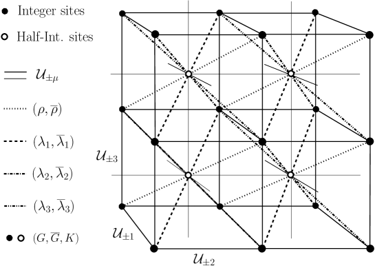
Fig. 3: All the configurations in $N=4\ D=3$ twisted SYM action for symmetric $a_{A}$

Fig. 4: Plaquettes

Fig. 5: Zero area loops

Fig. 6: Fermion loops in $N=4\ D=3$ twisted SYM action

The naïve continuum limit of the action (LABEL:N=4D=3action) can be taken through the expansion of gauge link variables (3.10). After using trace properties, one obtain the following continuum action,

$$S\rightarrow S_{cont} = \int d^{3}x\ \mathrm{tr}\ \biggl{[}\frac{1}{2}F_{\mu\nu}F_{\mu\nu}+K^{2}+G\overline{G}$$ (3.53)

$$-[\mathcal{D}_{\mu},\phi^{(\nu)}][\mathcal{D}_{\mu},\phi^{(\nu)}]-\frac{1}{2}[\phi^{(\mu)},\phi^{(\nu)}][\phi^{(\mu)},\phi^{(\nu)}]$$

$$-i\overline{\lambda}_{\mu}[\mathcal{D}_{\mu},\rho]-i\lambda_{\mu}[\mathcal{D}_{\mu},\overline{\rho}]+\epsilon_{\mu\nu\rho}\lambda_{\mu}[\mathcal{D}_{\nu},\overline{\lambda}_{\rho}]$$

$$-\overline{\lambda}_{\mu}[\phi^{(\mu)},\rho]-\lambda_{\mu}[\phi^{(\mu)},\overline{\rho}]+i\epsilon_{\mu\nu\rho}\lambda_{\mu}[\phi^{(\nu)},\overline{\lambda}_{\rho}]\biggr{]},$$

where $F_{\mu\nu}\equiv i[\mathcal{D}_{\mu},\mathcal{D}_{\nu}]$ represents the field strength with $\mathcal{D}_{\mu}\equiv\partial_{\mu}-iA_{\mu}$, while $\phi^{(\mu)}(\mu=1,2,3)$ denote three independent hermitian scalar fields in the twisted $N=4\ D=3$ SYM multiplet in the continuum spacetime. One could see that the kinetic term and potential term as well as Yukawa coupling terms for scalar fields naturally come up from the contributions of zero-area loops in the lattice action. The above action (3.53) have complete agreement with continuum construction of $N=4$ twisted SYM in three dimensions.

4 Discussions

A fully exact SUSY invariant formulation of twisted $N=4$ SYM action on three dimensional lattice is presented. Algebraic relations of Jacobi identities are geometrically realized on the simplicial lattice with the help of shift relations of component fields. The three dimensional lattice structure embedding the twisted $N=4$ SUSY naturally appears from the intrinsic relation between twisted fermions and Dirac-Kähler fermions. Twisted $N=4$ SUSY invariance is a natural consequence of the exact form of the action with respect to all the twisted supercharges up to surface terms which naturally vanish due to a trace property on the lattice.

Possible answers to the critiques on the formulation of link approach are given. It is pointed out that there is a proper ordering of a product of component fields which leads correct lattice SUSY transformation. We needed to introduce superparameters which anti-commute with all the supercovariant derivatives. It would be important to find an explicit representation of the super parameters. We further have to accept that a structure behind the nature of component fields which carry a shift and satisfy the relation (A-11) still remains to be better clarified. We consider that the lattice SUSY transformation can be defined only semilocally due to the next neighboring ambiguity of difference operation and thus gives influence on the ordering of component fields. Superfield may be able to take care of this semilocal nature of SUSY transformation faithfully[16].

In this paper we have not addressed the issue of hermiticity of the formulation. Although we haven’t yet reached to a complete understanding of hermitian property on odd dimensional lattice, it is possible to understand hermitian property and Majorana nature of fermion in two dimensional formulation[19]. We recognize that hermitian property of lattice SYM should also be understood from this perspective together with a better geometrical understandings of chirality on the lattice. It should also be mentioned that a dimensional reduction of three dimensional $N=4$ twisted SYM could give us a formulation of $N=4$ twisted SYM on two dimensional lattice, which corresponds to a double charged system of $N=D=2$ twisted SYM[19]. It is also important to proceed to perform a possible lattice formulation of $N=D=4$ Dirac-Kähler twisted SYM which should be carried out basically in the same manner as presented here. The results of these analyses will be given elsewhere.

Acknowledgments

We would like to thank to J. Kato, A. Miyake and J. Saito for useful discussions. This work is supported in part by Japanese Ministry of Education, Science, Sports and Culture under the grant number 18540245 and also by INFN research funds. I.K. is supported by the Special Postdoctoral Researchers Program at RIKEN. K.N. is supported by Department of Energy US Government, Grant No. FG02-91ER 40661.

APPENDIX

In this appendix we briefly discuss the argument given in [14] which according to the authors leads to an inconsistency in our lattice SUSY formulation with modified Leibniz rule and we show that there is no inconsistency at all. In this Appendix we consider, as in [14], only the case of the non-gauge version of lattice SUSY formulation. The lattice formulation of supersymmetric gauge theories, which is more relevant for the present paper and was criticized in [15], has been briefly discussed in Section 3.

Let us consider two superfields $\Phi_{i}(x,\theta_{A})$ ($i=1,2$) whose expansion into component fields is given by [1]:

$$\Phi_{1}(x,\theta_{A}) =\phi_{1}(x)+\theta_{A}\psi_{1}^{A}(x)+\cdots$$

$$\Phi_{2}(x,\theta_{A}) =\phi_{2}(x)+\theta_{A}\psi_{2}^{A}(x)+\cdots,.$$ (A-1)

Here we assume that the superfields $\Phi_{1}(x)$ and $\Phi_{2}(x)$ do not carry any shift while, according to [1], $\theta_{A}$ carry a shift opposite to that of the super charge $Q_{A}$ and thus $\psi_{A}$ carry the same shift $a_{A}$ as $Q_{A}$. The following notation will be used: given a superfield $\Phi(x,\theta_{A})$ we denote with $\Phi|_{0}(x)$ its first component, and by $\Phi|_{A}(x)$ the component corresponding to the coefficient of $\theta_{A}$ in the expansion. So for instance in (A-1) we have:

$$\Phi_{i}|_{0}(x)=\phi_{i}(x),~{}~{}~{}~{}~{}~{}~{}~{}~{}~{}~{}~{}~{}~{}~{}\Phi_{i}|_{A}(x)=\psi_{i}^{A}(x).$$ (A-2)

We define a super symmetry transformation $\delta_{A}=\eta_{A}Q_{A}$ (no sum) where $\eta_{A}$ is a supersymmetry parameter which carry the opposite shift of $Q_{A}$ so that the $\delta_{A}$ operation is shiftless. The SUSY transformation of the component fields can then be easily obtained, and we shall focus here on the transformation properties of the first component of a superfield (the argument can be extended to higher components)which reads:

$$\delta_{A}\Phi_{i}|_{0}(x)\equiv(\delta_{A}\Phi_{i})|_{0}(x)=\eta_{A}\Phi_{i}|_{A}(x),$$ (A-3)

that is, using (A-2)

$$\delta_{A}\phi_{i}(x)=\eta_{A}\psi_{i}^{A}(x).$$ (A-4)

According to [14] an inconsistency occurs when the SUSY variation of the product $\phi_{1}(x)\phi_{2}(x)$ is considered. Indeed if the variation $\delta_{A}(\phi_{1}\phi_{2})(x)$ is calculated using the modified Leibniz rule of eq. (2.13) the result will depend on the order of the two fields within the variation symbol in spite of the fact that they commute: of two super fields with a different order, we obtain

$$\delta_{A}(\phi_{1}(x)\phi_{2}(x)) =\eta_{A}(\psi_{1}^{A}(x)\phi_{2}(x)+\phi_{1}(x+a_{A})\psi_{2}^{A}(x)),$$

$$\delta_{A}(\phi_{2}(x)\phi_{1}(x)) =\eta_{A}(\psi_{2}^{A}(x)\phi_{1}(x)+\phi_{2}(x+a_{A})\psi_{1}^{A}(x)),$$ (A-5)

where we have used the following relation:

$$\phi_{i}(x)\eta_{A}=\eta_{A}\phi_{i}(x+a_{A}).$$ (A-6)

As a result the authors of [14] claim that ”there is an ambiguity in showing supersymmetry invariance of lattice actions” as a lattice action may be, or may be not, supersymmetric invariant depending on the order in which certain products of commuting component fields are written. In order to show that no ambiguity is really present we consider the product of the two superfields $\Phi_{1}$ and $\Phi_{2}$ and remark due to the noncommutativity between $\theta_{A}$ and the component fields as in (A-6), we have:

$$\Phi_{1}\Phi_{2}\neq\Phi_{2}\Phi_{1}.$$ (A-7)

The non-commutativity of the superfield product however does not apply to its lowest component (where no $\theta_{A}$ is involved) so that we have:

$$\Phi_{1}\Phi_{2}|_{0}(x)=\phi_{1}(x)\phi_{2}(x)=\phi_{2}(x)\phi_{1}(x)=\Phi_{2}\Phi_{1}|_{0}(x),$$ (A-8)

whereas we have

$$\Phi_{1}\Phi_{2}|_{A}(x)\neq\Phi_{2}\Phi_{1}|_{A}(x).$$ (A-9)

This is really the crucial point of the whole issue: $\phi_{1}(x)\phi_{2}(x)=\phi_{2}(x)\phi_{1}(x)$ can be seen as the first component of two (slightly) different superfields, namely $\Phi_{1}\Phi_{2}$ and $\Phi_{2}\Phi_{1}$. This does not happen in the continuum, where superfields commute and the first component identifies the superfield completely. We can now write the SUSY transformations (A-5), using the notation of (A-3):

$$\delta_{A}(\Phi_{1}\Phi_{2}|_{0}(x)) =\eta_{A}(\Phi_{1}\Phi_{2})|_{A}(x),$$

$$\delta_{A}(\Phi_{2}\Phi_{1}|_{0}(x)) =\eta_{A}(\Phi_{2}\Phi_{1})|_{A}(x).$$ (A-10)

There is no ambiguity in eq. (A-10) although the arguments of $\delta_{A}$ happen to coincide due to (A-8). In order to give an unambiguous meaning to (A-5) we have to agree that, although $\phi_{1}(x)$ and $\phi_{2}(x)$ commute and the numerical value of $\phi_{1}(x)\phi_{2}(x)$ and of $\phi_{2}(x)\phi_{1}(x)$ coincide, $\phi_{1}(x)\phi_{2}(x)$ (resp. $\phi_{2}(x)\phi_{1}(x)$) should be read as $\Phi_{1}\Phi_{2}|_{0}(x)$ (resp. $\Phi_{2}\Phi_{1}|_{0}(x)$) whenever used within a SUSY variation symbol $\delta_{A}$ in order to apply correctly the modified Leibniz rule. It should be noted that $\theta_{A}$ expansion of $\Phi_{1}\Phi_{2}$ and $\Phi_{2}\Phi_{1}$ have different expressions as a product of component fields except for the lowest component. This means that the order in which the component fields appear in the different terms of a Lagrangian is relevant if the correct SUSY transformation are to be reproduced via the modified Leibniz rule. We claim that one particular ordering is the correct one: the one that reflects in each term of the lagrangian the original order of the superfield product. Needless to say that if one uses the superfield formalism consistently the problem does not arise at all. It would be tempting then to require a complete commutativity of the superfields on the lattice. This could be achieved at the expense of introducing some non-commutativity between shifted component fields, namely:

$$\phi_{A}(x+a_{B})\phi_{B}(x)~{}~{}=~{}~{}(-1)^{|\phi_{A}||\phi_{B}|}\phi_{B}(x+a_{A})\phi_{A}(x),$$ (A-11)

where the fields $\phi_{A}$ and $\phi_{B}$ carry a shift $a_{A}$ and $a_{B}$, respectively. If (A-11) was satisfied the two expressions at the r.h.s. of (A-5) would coincide and any field order could be adopted in the lagrangian, starting from the ”correct” one, provided the coordinates were shifted according to (A-11). However, unless a concrete representation of $\phi_{A}(x)$ is found that satisfy (A-11), the condition above remains purely formal and difficult to use, say, within a functional integral.

References

• [1] A. D’Adda, I. Kanamori, N. Kawamoto and K. Nagata, Nucl. Phys. B707 (2005) 100 [hep-lat/0406029], Nucl. Phys. Proc. Suppl. 140 (2005) 754 [hep-lat/0409092], Nucl. Phys. Proc. Suppl. 140 (2005) 757.
• [2] A. D’Adda, I. Kanamori, N. Kawamoto and K. Nagata, Phys. Lett. B633 (2006) 645 [hep-lat/0507029].
• [3] P. Dondi and H. Nicolai, Nuovo Cim. A41 (1977) 1. S. Elitzur, E. Rabinovici and A. Schwimmer, Phys. Lett. B 199 (1982) 165. T. Banks and P. Windey, Nucl. Phys. B198 (1982) 226. S. Cecotti and L. Girardello, Nucl. Phys. B226 (1983) 417. N. Sakai and M. Sakamoto, Nucl. Phys. B229 (1983) 173. S. Elitzur and A. Schwimmer, Nucl. Phys. B226 (1983) 109. I. Ichinose, Phys. Lett. B122 (1983) 68. J. Bartels and J. B. Bronzan, Phys. Rev. D28 (1983) 818. J. Bartels and G. Kramer, Z. Phys. C20 (1983) 159. D. B. Kaplan, Phys. Lett. B136 (1984) 162. R. Nakayama and Y. Okada, Phys. Lett. B134 (1984) 241. S. Nojiri, Prog. Theor. Phys.  74 (1985) 819. G. Curci and G. Veneziano, Nucl. Phys. B292 (1987) 555. M. Golterman and D. Petcher, Nucl. Phys. B319 (1989) 307.
• [4] J. Nishimura, Phys. Lett. B406 (1997) 215 [hep-lat/9701013]. N. Maru and J. Nishimura, Int. J. Mod. Phys. A13 (1998) 2841 [hep-th/9705152]. H. Neuberger, Phys. Rev. D57 (1998) 5417 [hep-lat/9710089]. D. B. Kaplan and M. Schmaltz, Chin. J. Phys.  38 (2000) 543 [hep-lat/0002030]. G. T. Fleming, J. B. Kogut and P. M. Vranas, Phys. Rev. D64 (2001) 034510 [hep-lat/0008009]. I. Montvay, Int. J. Mod. Phys. A17 (2002) 2377 [hep-lat/0112007].
• [5] D. B. Kaplan, E. Katz and M. Ünsal, JHEP 0305 (2003) 037 [hep-lat/0206019]. A. G. Cohen, D. B. Kaplan, E. Katz and M. Ünsal, JHEP 0308 (2003) 024 [hep-lat/0302017]; JHEP 0312 (2003) 031 [hep-lat/0307012]. J. Nishimura, S. J. Rey and F. Sugino, JHEP 0302 (2003) 032 [hep-lat/0301025]. J. Giedt, E. Poppitz and M. Rozali, JHEP 0303 (2003) 035 [hep-th/0301048]. J. Giedt, Nucl. Phys. B668 (2003) 138 [hep-lat/0304006]; Nucl. Phys. B674 (2003) 259 [hep-lat/0307024]; Int. J. Mod. Phys.  A 21, 3039 (2006) [hep-lat/0602007]; [hep-lat/0605004] D. B. Kaplan and M. Unsal, JHEP 0509, 042 (2005) [hep-lat/0503039]. M. Unsal, JHEP 0511, 013 (2005) [hep-lat/0504016]; JHEP 0604, 002 (2006) [hep-th/0510004]. T. Onogi and T. Takimi, Phys. Rev.  D 72, 074504 (2005) [hep-lat/0506014]. M. G. Endres and D. B. Kaplan, JHEP 0610, 076 (2006) [hep-lat/0604012]. P. H. Damgaard and S. Matsuura, arXiv:0704.2696 [hep-lat].
• [6] W. Bietenholz, Mod. Phys. Lett. A14 (1999) 51 [hep-lat/9807010]. K. Fujikawa and M. Ishibashi, Nucl. Phys. B622 (2002) 115 [hep-th/0109156], Phys. Lett. B528 (2002) 295 [hep-lat/0112050]. Y. Kikukawa and Y. Nakayama, Phys. Rev. D66 (2002) 094508 [hep-lat/0207013]. K. Fujikawa, Phys. Rev. D66 (2002) 074510 [hep-lat/0208015]. M. Bonini and A. Feo, JHEP 0409 (2004) 011 [hep-lat/0402034]. J. W. Elliott and G. D. Moore, JHEP 0511, 010 (2005) [hep-lat/0509032].
• [7] S. Catterall and S. Karamov, Phys. Rev. D65 (2002) 094501 [hep-lat/0108024]; Phys. Rev. D68 (2003) 014503 [hep-lat/0305002]. S. Catterall, JHEP 0305 (2003) 038 [hep-lat/0301028]. S. Catterall and S. Ghadab, JHEP 0405 (2004) 044 [hep-lat/0311042], JHEP 0610, 063 (2006) [hep-lat/0607010]. S. Catterall, JHEP 0411 (2004) 006 [hep-lat/0410052]; JHEP 0506, 027 (2005) [hep-lat/0503036]; JHEP 0603 (2006) 032 [hep-lat/0602004]; JHEP 0704, 015 (2007) [hep-lat/0612008]. S. Catterall and T. Wiseman, arXiv:0706.3518 [hep-lat]. M. Hanada, J. Nishimura and S. Takeuchi arXiv:0706.1647 [hep-lat]. F. Sugino, JHEP 0401 (2004) 015 [hep-lat/0311021], JHEP 0403 (2004) 067 [hep-lat/0401017], JHEP 0501 (2005) 016 [hep-lat/0410035], Phys.Lett. B635 (2006) 218 [hep-lat/0601024]. M. Ünsal, JHEP 0610, 089 (2006) [hep-th/0603046]. K. Ohta and T. Takimi, Prog. Theor. Phys.  117, 317 (2007) [hep-lat/0611011]. T. Takimi, arXiv:0705.3831 [hep-lat]. P. H. Damgaard and S. Matsuura, arXiv:0706.3007 [hep-lat].
• [8] K. Itoh, M. Kato, H. Sawanaka, H. So and N. Ukita, JHEP 0302 (2003) 033 [hep-lat/0210049], Prog. Theor. Phys.  108 (2002) 363 [hep-lat/0112052].
• [9] A. Feo, Nucl. Phys. Proc. Suppl. 119 (2003) 198 [hep-lat/0112052], [hep-lat/0311037], and references therein. A. Feo, Mod. Phys. Lett. A 19 (2004) 2387 [hep-lat/0410012].
• [10] K. Fujikawa, Nucl. Phys. B636 (2002) 80 [hep-th/0205095].
• [11] H. Suzuki and Y. Taniguchi, JHEP 0510, 082 (2005) [hep-lat/0507019]. H. Suzuki, arXiv:0706.1392 [hep-lat]. Y. Kikukawa and H. Suzuki, JHEP 0502 (2005) 012 [hep-lat/0412042]. M. Harada and S. Pinsky, Phys. Rev. D 71 (2005) 065013 [hep-lat/0411024].
• [12] N. Kawamoto and T. Tsukioka, Phys. Rev. D61(2000)105009 [hep-th/9905222]. J. Kato, N. Kawamoto and Y. Uchida, Int. J. Mod. Phys. A 19(2004) 2149 [hep-th/0310242].
• [13] J. Kato, N. Kawamoto and A. Miyake, Nucl. Phys. B721 (2005) 229 [hep-th/0502119]. J. Kato and A. Miyake, Mod. Phys. Lett.  A 21, 2569 (2006) [hep-th/0512269].
• [14] F. Bruckmann and M. de Kok, Phys. Rev.  D 73, 074511 (2006) [hep-lat/0603003].
• [15] F. Bruckmann, S. Catterall and M. de Kok, Phys. Rev.  D 75, 045016 (2007) [hep-lat/0611001].
• [16] S. Arianos, A. D’Adda, N. Kawamoto and J. Saito, PoS(LATTICE 2007)259 [arXiv:0710.0487 [hep-lat]] and also to appear.
• [17] B. Geyer and D. Mulsch, Nucl. Phys. B616 (2001) 476 [hep-th/0108042].
• [18] I. Kanamori and N. Kawamoto, Int. J. Mod. Phys. A19 (2004) 695 [hep-th/0305094], Nucl. Phys. Proc. Suppl. 129 (2004) 877 [hep-lat/0309120].
• [19] A. D’Adda, I. Kanamori, N. Kawamoto, K. Nagata and J. Saito, to appear.