Separable and Low-Rank Continuous Games

Abstract

In this paper, we study nonzero-sum separable games, which are continuous games whose payoffs take a sum-of-products form. Included in this subclass are all finite games and polynomial games. We investigate the structure of equilibria in separable games. We show that these games admit finitely supported Nash equilibria. Motivated by the bounds on the supports of mixed equilibria in two-player finite games in terms of the ranks of the payoff matrices, we define the notion of the rank of an $n$-player continuous game and use this to provide bounds on the cardinality of the support of equilibrium strategies. We present a general characterization theorem that states that a continuous game has finite rank if and only if it is separable. Using our rank results, we present an efficient algorithm for computing approximate equilibria of two-player separable games with fixed strategy spaces in time polynomial in the rank of the game.

1 Introduction

The structure and computation of equilibria in games with infinite strategy spaces have long been recognized as complex. Even seemingly “good” games may possess only “bad” equilibria; Gross has constructed an example of a zero-sum game with rational utility functions whose unique Nash equilibrium is for each player to play the Cantor measure [11, 13]. To avoid such pathologies, Dresher, Karlin, and Shapley introduced the class of zero-sum separable games [9, 8, 14, 13]. These are games in which each player’s payoff can be written as a sum of products of functions in each player’s strategy separately (e.g. as polynomials), and it is known that every separable game admits a mixed strategy Nash equilibrium that is finitely supported, i.e. all players randomize over a finite number of pure strategies. Parrilo has shown that Nash equilibria of zero-sum games with polynomial utility functions can be computed efficiently [19].

In this paper, we study nonzero-sum separable games. We show that even in the nonzero-sum case, separable games have the property that an equilibrium exists in finitely supported mixed strategies. We then characterize the structure of these games and their Nash equilibria, and also propose methods for computing (exact and approximate) equilibria.

Our first major contribution is to define and develop the concept of the rank of a continuous game, which we use to construct bounds on the number of strategies played in equilibrium. In two-player finite games, Lipton et al. have recently shown that the ranks of the payoff matrices provide such a bound [16]. Our new definition of rank generalizes this one to allow for an arbitrary finite number of players (a problem explicitly left open in [16]) and infinite strategy spaces. We define the rank of a continuous game by introducing an equivalence relation between mixed strategies called almost payoff equivalence. The rank is the dimension of the mixed strategy space modulo this equivalence relation. Loosely speaking, low-rank continuous games are those where the variation in each player’s payoff depends only on a low-dimensional projection of the mixed strategies of the players. For example in games with polynomial payoffs, the rank depends on the dimension of a projection of the moment space.

We also show that a continuous game has finite rank if and only if it is separable. This means that little can be said about the structure of equilibria in non-separable continuous games and highlights the importance of separable games. We provide simple techniques for evaluating the rank of separable games, which we specialize to games with polynomial payoffs and finite games.

Our second set of results concern efficient computation of mixed strategy equilibria in separable games. For $n$-player games, we provide a nonlinear optimization formulation, and show that the optimal solutions of this problem correspond to the (generalized) moments of exact Nash equilibria. This formulation generalizes the optimization formulation of Nash equilibria of finite games presented by Başar and Olsder [1].

While the nonlinear optimization formulation for the computation of equilibria is tractable for certain classes of separable games such as zero-sum polynomial games, the potential nonconvexity of the optimization problem makes it impractical in other cases. We therefore supplement our computational results for exact mixed strategy equilibria with new methods for computing approximate mixed strategy equilibria. Using our rank results described above, we can link the computation of mixed strategy equilibria to the appropriate discretization of the strategy space into finite actions. For two-person separable games, this yields an efficient algorithm for computing approximate mixed strategy equilibria in time polynomial in the rank of the game. This algorithm searches for finitely supported approximate equilibria by enumerating all possible supports, and relies on the fact that the search can be limited to supports of size bounded by the rank of the game. For two-players, the set of equilibria for a given support can be described by linear equations and inequalities .

Our work is related to a number of literatures. There has been considerable work on the computation of equilibria in finite games. Lemke and Howson give a path-following algorithm for two-player finite games which can be viewed as the simplex method for linear programming operating with a different pivoting rule [15]. To find equilibria of games with more players, Scarf constructs a simplicial subdivision algorithm which also works for more general fixed point problems [22]. These methods rely on the polyhedral structure of the mixed strategy spaces of finite games, therefore they seem unlikely to generalize to continuous/separable games. For a survey of algorithms which compute equilibria of finite games, see [17].

Another growing literature has been investigating the complexity of computing mixed strategy Nash equilibria of finite games. Daskalakis, Goldberg, and Papadimitriou settle this question for finite normal form games with four or more players, showing that the problem of computing a single Nash equilibrium is PPAD-complete [6]. In essence this means that it is computationally equivalent to a number of other fixed point problems which are believed to be computationally difficult. These problems share the feature that a solution can be proven to exist, but the known proofs of existence are inefficient; for more about the complexity class PPAD, see [18]. Daskalakis and Papadimitriou later improve this result by proving PPAD-completeness in the case of three players [7]. Chen and Deng also prove this independently [4] and complete this line of work by proving PPAD-completeness for two players [5]. In this literature, there has been no work on continuous games.

Our work is most closely related to the work of Lipton et al. [16], who consider two-player finite games and provide bounds on the support of equilibrium strategies using the ranks of the payoff matrices of the players. Since finite games are a special case of separable games, our results on the cardinality of the support of equilibrium strategies generalize theirs by allowing for an arbitrary finite number of players as well as infinite strategy sets and a broader class of payoff functions.

Lipton et al. also investigate computing approximate equilibria in two-player finite games and present the first algorithm for computing approximate equilibria which is quasi-polynomial in the number of strategies [16]. The rank of a separable game measures the complexity of the payoffs, and in the case of a finite game it is bounded by the number of strategies. Therefore in finite games the complexity of the payoffs and the complexity of the strategy spaces do not vary independently; the effects of these parameters on the running time of algorithms cannot be distinguished. However, for games with infinite strategy sets the rank can be varied arbitrarily while the strategy set is held fixed. This allows us to construct an algorithm for computing approximate equilibria in two-player separable games with fixed (infinite) strategy spaces and show that it has a polynomial dependence on the rank. Since we assume the strategy space is fixed and consider general separable games rather than only finite games, our algorithm is not directly comparable to that of Lipton et al. [16]. Nonetheless it is interesting on its own since no algorithm for computing approximate equilibria of finite games is known which has polynomial dependence on the complexity of the game.

Our work is also related to that of Kannan and Theobald, who study a different notion of rank in two-player finite games [12]. They take an algorithmic perspective and view zero-sum games as the simplest type of games. To generalize these, they propose a hierarchy of classes of two-player finite games in which the rank of the sum $R+C$ of the payoff matrices is bounded by a constant $k$; the case $k=0$ corresponds to zero-sum games. For fixed $k$, they show that approximate Nash equilibria of two-player finite games can be computed in time polynomial in the description length for the game. This algorithm relies on an approximation result for quadratic programming due to Vavasis [25] which depends on the polyhedral structure of the problem. It is conceivable that this technique may apply to polynomial games if the approximation technique can be extended to this more general algebraic setting, but we do not do so here.

The rest of this paper is organized as follows. In Section 2 we define separable games and prove some of their basic properties. Then in Section 3 we define the rank of a continuous game and use this definition to bound the cardinality of the support of Nash equilibria. We present a characterization theorem for separable games which in particular shows that within the class of continuous games, the low-rank results in this paper cannot be extended past separable games. We provide a simple formula for computing the rank of arbitrary separable games, which we specialize for finite and polynomial games. In Section 4 we discuss computation of Nash equilibria and approximate equilibria. We close with conclusions and directions for future work.

2 Basic Theory of Separable Games

We first introduce the notational conventions and the basic terminology used throughout the paper. Subscripts refer to players, while superscripts are reserved for other indices, rather than exponents. If $S_{j}$ are sets for $j=1,\ldots,n$ then $S=\Pi_{j=1}^{n}S_{j}$ and $S_{-i}=\Pi_{j\neq i}S_{j}$. The $n$-tuple $s$ and the $(n-1)$-tuple $s_{-i}$ are formed from the points $s_{j}$ similarly. Given a subset $S$ of a vector space, we use the notation $\operatorname{span}S$, $\operatorname{aff}S$, $\operatorname{conv}S$, and $\overline{S}$ to denote the span, affine hull, convex hull, and closure of the set $S$, respectively. We denote the transpose of a matrix $M$ by $M^{\prime}$.

Definition 2.1.

An $n$-player continuous game consists of a pure strategy space $C_{i}$ which is a nonempty compact metric space and a continuous utility or payoff function $u_{i}:C\rightarrow\mathbb{R}$ for each player $i=1,\ldots,n$. Throughout, $\Delta_{i}$ will denote the space of Borel probability measures $\sigma_{i}$ over $C_{i}$, referred to as mixed strategies, and the $u_{i}$ will be extended from $C$ to $\Delta$ by expectation, defining

$$u_{i}(\sigma)=\int_{C}u_{i}(s)d\sigma,$$

where the $n$-tuple $\sigma=(\sigma_{1},\ldots,\sigma_{n})$ is identified with the product measure $\sigma_{1}\times\cdots\times\sigma_{n}$.

Definition 2.2.

An $n$-player separable game is an $n$-player continuous game with utility functions $u_{i}:C\rightarrow\mathbb{R}$ taking the form

$$u_{i}(s)=\sum_{j_{1}=1}^{m_{1}}\cdots\sum_{j_{n}=1}^{m_{n}}a_{i}^{j_{1}\cdots j_{n}}f_{1}^{j_{1}}(s_{1})\cdots f_{n}^{j_{n}}(s_{n}),$$ (1)

where $a_{i}^{j_{1}\cdots j_{n}}\in\mathbb{R}$ and the $f_{i}^{j}:C_{i}\rightarrow\mathbb{R}$ are continuous. Two important special cases are the finite games in which the $C_{i}$ are finite and the $u_{i}$ are arbitrary and the polynomial games in which the $C_{i}$ are compact intervals in $\mathbb{R}$ and the $u_{i}$ are polynomials in the $s_{j}$.

When it is convenient to do so, and always for polynomial games, we will begin the summations in (1) at $j_{i}=0$. For polynomial games we can then use the convention that $f_{i}^{j}(s_{i})=s_{i}^{j}$, where the superscript on the right hand side denotes an exponent rather than an index.

Example 2.3.

Consider a two player game with $C_{1}=C_{2}=[-1,1]\subset\mathbb{R}$. Letting $x$ and $y$ denote the pure strategies of players $1$ and $2$, respectively, we define the utility functions

$$\begin{split}u_{1}(x,y)&=2xy+3y^{3}-2x^{3}-x-3x^{2}y^{2}\text{\ \ and}\\ u_{2}(x,y)&=2x^{2}y^{2}-4y^{3}-x^{2}+4y+x^{2}y.\end{split}$$ (2)

This is a polynomial game, and we will return to it periodically to apply the results presented. In particular, we will show using classical techniques that this game must have a Nash equilibrium in which each player randomizes over a set of cardinality at most $5$. We will then apply our new rank results (see Theorem 3.3) to reduce this bound to $2$ for the first player and $4$ for the second player.

Let $V_{i}$ denote the space of all finite-valued signed measures (henceforth simply called measures) on $C_{i}$, which can be identified with the dual of the Banach space $C(C_{i})$ of all continuous real-valued functions on $C_{i}$ endowed with the sup norm. Throughout, we will use the weak* topology on $V_{i}$, which is the weakest topology such that whenever $f:C_{i}\rightarrow\mathbb{R}$ is a continuous function, $\sigma\mapsto\int fd\sigma$ is a continuous linear functional on $V_{i}$.

We can extend the utility functions of a continuous game to all of $V$ in the same way they are extended from $C$ to $\Delta$, yielding a multilinear functional on $V$. For a fixed separable game we can extend the $f_{i}^{j}$ from $C_{i}$ to $V_{i}$ similarly, yielding the so-called generalized moment functionals, so (1) holds with $s$ replaced by $\sigma\in V$. In polynomial games $f_{i}^{j}(s_{i})=s_{i}^{j}$ so the generalized moment functionals are just the classical moment functionals. We will abuse notation and identify the elements of $C_{i}$ with the atomic measures in $\Delta_{i}$, so $C_{i}\subseteq\Delta_{i}\subset V_{i}$. Note that $\operatorname{conv}C_{i}$ and $\operatorname{span}C_{i}$ are the set of all finitely supported probability measures and the set of all finitely supported finite signed measures, respectively. The following are standard results (see [20] and [21]).

Proposition 2.4.

• The sets $C_{i}$ and $\Delta_{i}$ are weak* compact.

• The weak* closures of $\operatorname{conv}C_{i}$ and $\operatorname{span}C_{i}$ are $\Delta_{i}$ and $V_{i}$, respectively.

• The weak* topology makes $V_{i}$ a Hausdorff topological vector space.

We next define three notions of equivalence between two measures, which allow us to exhibit simplifications in the structure of Nash equilibria in separable games.

Definition 2.5.

Two measures $\sigma_{i},\tau_{i}\in V_{i}$ are

• moment equivalent if $f_{i}^{j}(\sigma_{i})=f_{i}^{j}(\tau_{i})$ for all $j$ (representation-dependent and only defined for separable games).

• payoff equivalent if $u_{j}(\sigma_{i},s_{-i})=u_{j}(\tau_{i},s_{-i})$ for all $j$ and all $s_{-i}\in C_{-i}$.

• almost payoff equivalent if $u_{j}(\sigma_{i},s_{-i})=u_{j}(\tau_{i},s_{-i})$ for all $j\neq i$ and all $s_{-i}\in C_{-i}$.

Note that in separable games moment equivalence implies payoff equivalence and in all continuous games payoff equivalence implies almost payoff equivalence. Since the $f_{i}^{j}$ and $u_{j}$ are linear and multilinear functionals on $V_{i}$ and $V$, respectively, these equivalence relations can be expressed in terms of (potentially infinitely many) linear constraints on $\sigma_{i}-\tau_{i}$.

Definition 2.6.

Let $0$ denote the zero measure in $V_{i}$ and define

• $W_{i}=\left\{\text{measures moment equivalent to }0\right\}$,

• $X_{i}=\left\{\text{measures payoff equivalent to }0\right\}$,

• $Y_{i}=\left\{\text{measures almost payoff equivalent to }0\right\}$.

Then $W_{i}\subseteq X_{i}\subseteq Y_{i}$, and $\sigma_{i}-\tau_{i}\in X_{i}$ if and only if $\sigma_{i}$ is payoff equivalent to $\tau_{i}$, etc. Furthermore, the subspaces $X_{i}$ and $Y_{i}$ are representation-independent and well-defined for any continuous game, separable or not. Note that these subspaces are given by the intersection of the kernels of (potentially infinitely many) continuous linear functionals, hence they are closed.

We will analyze separable games by considering the quotients of $V_{i}$ by these subspaces, i.e. $V_{i}$ mod these three equivalence relations. To avoid defining excessively many symbols let $\Delta_{i}/W_{i}$ denote the image of $\Delta_{i}$ in $V_{i}/W_{i}$ and so forth. For a concrete example of these sets see the discussion at end of this section, and in particular Figure 1.

The following theorem presents a fundamental result about separable games. It shows that regardless of the choices of the other players, each player is free to restrict his choice of strategies to a particularly simple class of mixed strategies, namely those which only assign positive probability to a finite number of pure strategies. Furthermore, a bound on the number of strategies needed can be easily computed in terms of the structure of the game. This theorem can be proven by a separating hyperplane argument as applied to zero-sum separable games by Karlin [13], but here we give a new topological argument.

Theorem 2.7.

In a separable game every mixed strategy $\sigma_{i}$ is moment equivalent to a finitely-supported mixed strategy $\tau_{i}$ with $|\operatorname{supp}(\tau_{i})|\leq m_{i}+1$. Moreover, if $\sigma_{i}$ is countably-supported $\tau_{i}$ can be chosen with $\operatorname{supp}(\tau_{i})\subset\operatorname{supp}(\sigma_{i})$.

Proof.

Note that the map

$$f_{i}:\sigma_{i}\mapsto\left(f_{i}^{1}(\sigma_{i}),\ldots,f_{i}^{m_{i}}(\sigma_{i})\right)$$ (3)

is linear and continuous. Therefore

$$f_{i}(\Delta_{i})=f_{i}\left(\overline{\operatorname{conv}C_{i}}\right)\subseteq\overline{f_{i}(\operatorname{conv}C_{i})}=\overline{\operatorname{conv}f_{i}(C_{i})}=\operatorname{conv}f_{i}(C_{i})=f_{i}(\operatorname{conv}C_{i})\subseteq f_{i}(\Delta_{i}).$$

The first three steps follow from Proposition 2.4, continuity of $f_{i}$, and linearity of $f_{i}$, respectively. The next equality holds because $\operatorname{conv}f_{i}(C_{i})$ is compact, being the convex hull of a compact subset of a finite-dimensional space. The final two steps follow from the linearity of $f_{i}$ and the containment $\operatorname{conv}C_{i}\subseteq\Delta_{i}$. Hence, we have

$$f_{i}(\Delta_{i})=\operatorname{conv}f_{i}(C_{i})=f_{i}(\operatorname{conv}C_{i}).$$

This shows that any mixed strategy is moment equivalent to a finitely-supported mixed strategy. Applying Carathéodory’s theorem [2] to the set $\operatorname{conv}f_{i}(C_{i})\subset\mathbb{R}^{m_{i}}$ yields the uniform bound. Since a countable convex combination of points in a bounded subset of $\mathbb{R}^{m_{i}}$ can always be written as a finite convex combination of at most $m_{i}+1$ of those points, the final claim follows. ∎

For the rest of the paper we will study the Nash equilibria of (nonzero-sum) separable games, which are defined for arbitrary continuous games as follows.

Definition 2.8.

A mixed strategy profile $\sigma$ is a Nash equilibrium if $u_{i}(\tau_{i},\sigma_{-i})\leq u_{i}(\sigma)$ for all $i$ and all $\tau_{i}\in\Delta_{i}$.

Combining Theorem 2.7 with Glicksberg’s result [10] that every continuous game has a Nash equilibrium yields the following:

Corollary 2.9.

Every separable game has a Nash equilibrium in which player $i$ mixes among at most $m_{i}+1$ pure strategies.

Example 2.3 (cont’d).

Apply the standard definition of the $f_{i}^{j}$ to the polynomial game with payoffs given in (2). The set of moments $\Delta_{i}/W_{i}\cong f_{i}(\Delta_{i})$ as described in Theorem 2.7 is shown in Figure 1 with the zeroth moment omitted (it is identically unity). In this case the set of moments is the same for both players. The space $V_{i}/W_{i}=f_{i}(V_{i})$ is a four-dimensional real vector space, and Figure 1 shows a subset of the projection of $V_{i}/W_{i}$ onto its final three coordinates. The set $C_{i}/W_{i}=f_{i}(C_{i})$ of moments due to pure strategies is the curve traced out by the vector $(1,x,x^{2},x^{3})$ as $x$ varies from $-1$ to $1$. Since the first coordinate is omitted in the figure, this can be seen as the sharp edge which goes from $(-1,1,-1)$ through $(0,0,0)$ to $(1,1,1)$. As shown in the proof of Theorem 2.7, $f_{i}(\Delta_{i})$ is exactly the convex hull of this curve.

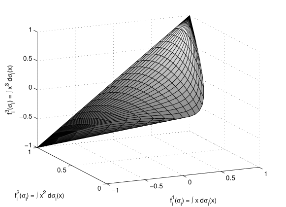
Figure 1: The space $f_{i}(\Delta_{i})\cong\Delta_{i}/W_{i}$ of possible moments for either player’s mixed strategy under the payoffs given in (2) due to a measure $\sigma_{i}$ on $[-1,1]$. The zeroth moment, which is identically unity, has been omitted.

For each player the range of the indices in (1) is $0\leq j_{i}\leq 3$, so by Corollary 2.9, this game has an equilibrium in which each player mixes among at most $4+1=5$ pure strategies. To produce this bound, we have not used any information about the payoffs except for the degree of the polynomials. However, notice that there is extra structure here to be exploited. For example, $u_{2}$ depends on the expected value $\int x^{2}d\sigma_{1}(x)$, but not on $\int xd\sigma_{1}(x)$ or $\int x^{3}d\sigma_{1}(x)$. In particular, player $2$ is indifferent between the two strategies $\pm x$ of player $1$ for all $x$, insofar as this choice does not affect his payoff (though it does affect what strategy profiles are equilibria). In the following section, we will present improved bounds on the number of strategies played in an equilibrium which take these simplifications into account in a systematic manner.

3 The Rank of a Continuous Game

In this section, we introduce the notion of the rank of a continuous game. We use this notion to provide improved bounds on the cardinality of the support of the equilibrium strategies for a separable game. We also provide a characterization theorem which states that a continuous game has finite rank if and only if it is separable, thus showing that separable games are the largest class of continuous games to which low-rank arguments apply (see subsection 3.2). We conclude this section by showing how to compute the rank of a separable game in Subsection 3.3, which may be read independently of the section on the characterization theorem.

Our main result on bounding the support of equilibrium strategies generalizes the following theorem of Lipton et al. [16] to arbitrary separable games, thereby removing the two-player assumption and weakening the restriction that the strategy spaces be finite. The proof given in [16] is essentially an algorithmic version of Carathéodory’s theorem. Here we provide a shorter nonalgorithmic proof which illustrates some of the ideas to be used in establishing the extended version of the theorem.

Theorem 3.1 (Lipton et al. [16]).

Consider a two-player finite (i.e. bimatrix) game defined by matrices $R$ and $C$ of payoffs to the row and column player, respectively. Let $\sigma$ be a Nash equilibrium of the game. Then there exists a Nash equilibrium $\tau$ which yields the same payoffs to both players as $\sigma$, but in which the column player mixes among at most $\operatorname{rank}R+1$ pure strategies and the row player mixes among at most $\operatorname{rank}C+1$ pure strategies.

Proof.

Let $r$ and $c$ be probability column vectors corresponding to the mixed strategies of the row and column players in the given equilibrium $\sigma$. Then the payoffs to the row and column players are $r^{\prime}Rc$ and $r^{\prime}Cc$. Since $c$ is a probability vector, we can view $Rc$ as a convex combination of the columns of $R$. These columns all lie in the column span of $R$, which is a vector space of dimension $\operatorname{rank}R$. By Carathéodory’s theorem, we can therefore write any convex combination of these vectors using only $\operatorname{rank}R+1$ terms [2]. That is to say, there is a probability vector $d$ such that $Rd=Rc$, $d$ has at most $\operatorname{rank}R+1$ nonzero entries, and a component of $d$ is nonzero only if the corresponding component of $c$ was nonzero.

Since $r$ was a best response to $c$ and $Rc=Rd$, $r$ is a best response to $d$. On the other hand, since $(r,c)$ was a Nash equilibrium $c$ must have been a mixture of best responses to $r$. But $d$ only assigns positive probability to strategies to which $c$ assigned positive probability. Thus $d$ is a best response to $r$, so $(r,d)$ is a Nash equilibrium which yields the same payoffs to both players as $(r,c)$, and $d$ only assigns positive probability to $\operatorname{rank}R+1$ pure strategies. Applying the same procedure to $r$ we could find an $s$ which only assigns positive probability to $\operatorname{rank}C+1$ pure strategies and such that $(s,d)$ is a Nash equilibrium with the same payoffs to both players as $(r,c)$. ∎

We will show in the following subsection that our extension of this theorem provides a slightly tighter bound of $\operatorname{rank}R$ instead of $\operatorname{rank}R+1$ (respectively for $C$) in some cases, depending on the structure of $R$ and $C$. This can be seen directly from the proof given here. We considered convex combinations of the columns of $R$ and noted that these all lie in the column span of $R$. In fact, they all lie in the affine hull of the set of columns of $R$. If this affine hull does not include the origin, then it will have dimension $\operatorname{rank}R-1$. The rest of the proof goes through using this affine hull instead of the column span, and so in this case we get a bound of $\operatorname{rank}R$ on the number of strategies played with positive probability by the row player. Alternatively, the dimension of the affine hull can be computed directly as the rank of the matrix given by subtracting a fixed column of $R$ from all the other columns of $R$.

3.1 Bound on the Support of Equilibrium Strategies

By comparing the two-player case of (1) with the singular value decomposition for matrices, separable games can be thought of as games of “finite rank.” Now we will define the rank of a continuous game precisely and use it to give a bound on the cardinality of the support of equilibrium strategies, generalizing Corollary 2.9 and Theorem 3.1. The primary tool will be the notion of almost payoff equivalence from Definition 2.5. In what follows, the dimension of a set will refer to the dimension of its affine hull.

Definition 3.2.

The rank of a continuous game is defined to be the $n$-tuple $\rho=(\rho_{1},\ldots,\rho_{n})$ where $\rho_{i}=\dim\Delta_{i}/Y_{i}$. A game is said to have finite rank if $\rho_{i}<\infty$ for all $i$.

Since $W_{i}\subseteq Y_{i}$ and $V_{i}/W_{i}$ is finite-dimensional for any separable game (see the proof of Theorem 2.7), it is clear that separable games have finite rank, and furthermore that $\rho_{i}\leq m_{i}$ for all $i$. In subsection 3.2 we show that all games of finite rank are also separable, so the two conditions are equivalent. Unlike the $m_{i}$, the rank is defined for all continuous games and is representation-independent.

We define the rank of a game in terms of almost payoff equivalence of mixed strategies by means of the subspace $Y_{i}$. This notion of equivalence between two strategies for a given player means that no matter what the other players do, their payoffs will not enable them to distinguish these two strategies. The use of this equivalence relation reflects the fact that at a (mixed strategy) Nash equilibrium, the payoff to a player is equalized among all pure strategies which he plays with positive probability. Therefore the player is free to switch to any other mixed strategy supported on the same pure strategies, as long as the change does not affect the other players, and the resulting strategy profile will remain a Nash equilibrium.

Using the rank of a game, Corollary 2.9 and Theorem 3.1 can now be improved as follows:

Theorem 3.3.

Given an equilibrium $\sigma$ of a separable game with rank $\rho$, there exists an equilibrium $\tau$ such that each player $i$ mixes among at most $\rho_{i}+1$ pure strategies and $u_{i}(\sigma)=u_{i}(\tau)$.

If $\dim\Delta_{i}/X_{i}=1$ and the metric space $C_{i}$ is connected, then this bound can be improved so that $\tau_{i}$ is a pure strategy.

Proof.

By Theorem 2.7, we can assume without loss of generality that each player’s mixed strategy $\sigma_{i}$ is finitely supported. Fix $i$, let $\psi_{i}:V_{i}\rightarrow V_{i}/Y_{i}$ denote the canonical projection transformation and let $\sigma_{i}=\sum_{j}\lambda^{j}s_{i}^{j}$ be a finite convex combination of pure strategies. By linearity of $\psi_{i}$ we have

$$\psi_{i}(\sigma_{i})=\sum_{j}\lambda^{j}\psi_{i}(s_{i}^{j}).$$

Carathéodory’s theorem states that (renumbering the $s_{i}^{j}$ and adding some zero terms if necessary) we can write

$$\psi_{i}(\sigma_{i})=\sum_{j=0}^{\rho_{i}}\mu^{j}\psi_{i}(s_{i}^{j}),$$

a convex combination potentially with fewer terms. Let $\tau_{i}=\sum_{j=0}^{\rho_{i}}\mu^{j}s_{i}^{j}$. Then $\psi_{i}(\sigma_{i})=\psi_{i}(\tau_{i})$. Since $\sigma$ was a Nash equilibrium, and $\sigma_{i}$ is almost payoff equivalent to $\tau_{i}$, $\sigma_{j}$ is a best response to $(\tau_{i},\sigma_{-i,j})$ for all $j\neq i$. On the other hand $\sigma_{i}$ was a mixture among best responses to the mixed strategy profile $\sigma_{-i}$, so the same is true of $\tau_{i}$, making it a best response to $\sigma_{-i}$. Thus $(\tau_{i},\sigma_{-i})$ is a Nash equilibrium.

If $\dim\Delta_{i}/X_{i}=1$ and $C_{i}$ is connected, then $C_{i}/X_{i}$ is connected, compact, and one-dimensional, i.e. it is an interval.  Therefore it is convex, so $\Delta_{i}/X_{i}=\operatorname{conv}(C_{i}/X_{i})=C_{i}/X_{i}$. This implies that there exists a pure strategy $s_{i}$ which is payoff equivalent to $\sigma_{i}$, so we may take $\tau_{i}=s_{i}$ and $(\tau_{i},\sigma_{-i})$ is a Nash equilibrium.

Beginning with this equilibrium and repeating the above steps for each player in turn completes the construction of $\tau$ and the final statement of the theorem is clear. ∎

While the preceding theorem was the original reason for our choice of the definition of $\rho$, the definition turns out to have other interesting properties which we study below. The following alternative characterization of the rank of a continuous game is more concrete than the definition given above. This theorem simplifies the proofs of many rank-related results and will be applied to the problem of computing the rank of separable games in Subsection 3.3.

Theorem 3.4.

The rank $\rho_{i}$ for player $i$ in a continuous game is given by the smallest $r_{i}$ such that there exist continuous functions $g_{i}^{k}:C_{i}\rightarrow\mathbb{R}$ and $h_{i,j}^{k}:C_{-i}\rightarrow\mathbb{R}$ which satisfy

$$u_{j}(s)=h_{i,j}^{0}(s_{-i})+\sum_{k=1}^{r_{i}}g_{i}^{k}(s_{i})h_{i,j}^{k}(s_{-i})$$ (4)

for all $s\in C$ and $j\neq i$ ($\rho_{i}=\infty$ if and only if no such representation exists). Furthermore, the minimum value of $r_{i}=\rho_{i}$ is achieved by functions $g_{i}^{k}(s_{i})$ of the form $u_{j}(s_{i},s_{-i})$ for some $s_{-i}\in C_{-i}$ and $j\neq i$ and functions $h_{i,j}^{k}(s_{-i})$ of the form $\int u_{j}(\cdot,s_{-i})d\sigma_{i}$ for some $\sigma_{i}\in V_{i}$.

Proof.

Throughout the proof we will automatically extend any functions $g_{i}^{k}:C_{i}\rightarrow\mathbb{R}$ to all of $V_{i}$ in the canonical way. Suppose we are given a representation of the form (4). Let $g_{i}:C_{i}\rightarrow\mathbb{R}^{r_{i}}$ be defined by $g_{i}(s_{i})=\left(g_{i}^{1}(s_{i}),\ldots,g_{i}^{r_{i}}(s_{i})\right)$. By definition, $\rho_{i}$ is the dimension of $\Delta_{i}/Y_{i}$. Let $Z_{i}$ denote the subspace of $V_{i}$ parallel to $\Delta_{i}$, i.e. the space of all signed measures $\sigma_{i}$ such that $\int\sigma_{i}=0$. Then $\rho_{i}=\dim Z_{i}/(Z_{i}\cap Y_{i})$. By (4) any signed measure which is in $Z_{i}$ and in $\operatorname{ker}g_{i}$ is almost payoff equivalent to the zero measure, so $Z_{i}\cap\operatorname{ker}g_{i}\subseteq Z_{i}\cap Y_{i}$ and therefore

$$\rho_{i}=\dim Z_{i}/(Z_{i}\cap Y_{i})\leq\dim Z_{i}/(Z_{i}\cap\operatorname{ker}g_{i})=\dim g_{i}(Z_{i})\leq r_{i}.$$

It remains to show that if $\rho_{i}<\infty$ then there exists a representation of the form (4) with $r_{i}=\rho_{i}$. Recall that $Y_{i}$ is defined to be

$$Y_{i}=\bigcap_{\stackrel{{\scriptstyle j\neq i}}{{s_{-i}\in C_{-i}}}}\operatorname{ker}u_{j}(\cdot,s_{-i})$$

where $u_{j}(\cdot,s_{-i})$ is interpreted as a linear functional on $V_{i}$. Since $\rho_{i}=\dim Z_{i}/(Z_{i}\cap Y_{i})$, we can choose $\rho_{i}$ linear functionals, call them $g_{i}^{1},\ldots,g_{i}^{\rho_{i}}$, from the collection of functionals whose intersection forms $Y_{i}$, such that $Z_{i}\cap Y_{i}=Z_{i}\cap\operatorname{ker}g_{i}$, where $g_{i}=(g_{i}^{1},\ldots,g_{i}^{\rho_{i}})$ as above. We cannot choose a smaller collection of linear functionals and achieve $Z_{i}\cap Y_{i}=Z_{i}\cap\operatorname{ker}g_{i}$, because $\rho_{i}=\dim Z_{i}/(Z_{i}\cap Y_{i})$. Note that $Z_{i}\cap\operatorname{ker}g_{i}=\operatorname{ker}\left(1,g_{i}^{1},\ldots,g_{i}^{\rho_{i}}\right)$ where $1$ is the linear functional $1(\sigma_{i})=\int d\sigma_{i}$. Therefore no functional can be removed from the list $(1,g_{i})=(1,g_{i}^{1},\ldots,g_{i}^{\rho_{i}})$ without affecting the kernel of the transformation $(1,g_{i})$, so the functionals $1,g_{i}^{1},\ldots,g_{i}^{\rho_{i}}$ are linearly independent.

This means that any of the linear functionals $u_{j}(\cdot,s_{-i})$ (the intersection of whose kernels yields $Y_{i}$) can be written uniquely as a linear combination of the functionals $1,g_{i}^{1},\ldots,g_{i}^{\rho_{i}}$. That is to say, there are unique functions $h_{i,j}^{k}$ such that (4) holds with the functions $g_{i}^{k}$ constructed here and $r_{i}=\rho_{i}$. The $g_{i}^{k}$ are continuous by construction, so to complete the proof we must show that the functions $h_{i,j}^{k}$ are continuous as well. Since the functionals $1,g_{i}^{1},\ldots,g_{i}^{\rho_{i}}$ are linearly independent, we can choose a measure $\sigma_{i}^{k}\in V_{i}$ which makes the $k^{\text{th}}$ of these functionals evaluate to unity and all the others zero. Substituting these values into (4) shows that $h_{i,j}^{k}(s_{-i})=\int u_{j}(\cdot,s_{-i})d\sigma_{i}^{k}$. Since $u_{j}$ is continuous, $h_{i,j}^{k}$ is therefore also continuous. ∎

Note that in the statement of Theorem 3.4 we have distinguished the component $h_{i,j}^{0}(s_{-i})$ in $u_{j}$. We have shown that this distinction follows from the definition of $\rho_{i}$, but there is also an intuitive game theoretic reason why this separation is natural.  As mentioned above, $\rho_{i}$ is intended to capture the number of essential degrees of freedom that player $i$ has in his choice of strategy when playing a Nash equilibrium. Theorems 3.3 and 3.4 together show that player $i$ only needs to take the other players’ utilities into account to compute this number, and not his own. But player $i$ is only concerned with the other players’ utilities insofar as his own strategic choice affects them. The function $h_{i,j}^{0}(s_{-i})$ captures the part of player $j$’s utility which does not depend on player $i$’s strategy, so whether this function is zero or not it has no effect on the rank $\rho_{i}$.

Also note that while Theorem 3.4 gives decompositions of the utilities in terms of the $\rho_{i}$, it is not in general possible to summarize all these decompositions by writing the utilities in the form (1) with $m_{i}=\rho_{i}$ for all $i$. For a trivial counterexample, consider any game in which $u_{i}(s)=h_{i}^{0}(s_{-i})$ is independent of $s_{i}$ for all $i$. Then Theorem 3.4 implies that $\rho_{i}=0$ for all $i$, but the utilities are nonzero so we cannot take $m_{i}=0$ in (1) for any $i$.

We close this subsection with an application. If a submatrix is formed from a matrix by “sampling,” i.e. selecting a subset of the rows and columns, the rank of the submatrix is bounded by the rank of the original matrix. Theorem 3.4 shows that the same is true of continuous games, because a factorization of the form (4) for a game immediately provides a factorization for any smaller game produced by restricting the players’ choices of strategies.

Corollary 3.5.

Let $(\{C_{i}\},\{u_{i}\})$ be a continuous game with rank $\rho$ and $\tilde{C}_{i}$ be a nonempty compact subset of $C_{i}$ for each $i$, with $\tilde{u}_{i}=u_{i}\big{|}_{\tilde{C}}$. Let $\tilde{\rho}$ denote the rank of the game $(\{\tilde{C}_{i}\},\{\tilde{u}_{i}\})$. Then we have $\tilde{\rho}_{i}\leq\rho_{i}$ for all $i$.

Definition 3.6.

The game $(\{\tilde{C}_{i}\},\{\tilde{u}_{i}\})$ in Corollary 3.5 is called a sampled game or a sampled version of $(\{C_{i}\},\{u_{i}\})$.

Note that if we take $\tilde{C}_{i}$ to be finite for each $i$, then the sampled game is a finite game. If the original game is separable and hence has finite rank, then Corollary 3.5 yields a uniform bound on the complexity of finite games which can arise from this game by sampling. This fact is applied to the problem of computing approximate equilibria in Section 4 below. Finally, note that there are other kinds of bounds on the cardinality of the support of equilibria (e.g., for special classes of polynomial games as studied by Karlin [13]) which do not share this sampling property.

3.2 Characterizations of separable games

In this section we present a characterization theorem for separable games. We also provide an example that shows that the assumptions of this theorem cannot be weakened.

Theorem 3.7.

For a continuous game, the following are equivalent:

1. The game is separable.

2. The game has finite rank.

3. For each player $i$, every countably supported mixed strategy $\sigma_{i}$ is almost payoff equivalent to a finitely supported mixed strategy $\tau_{i}$ with $\operatorname{supp}(\tau_{i})\subset\operatorname{supp}(\sigma_{i})$.

To prove that finite rank implies separability we repeatedly apply Theorem 3.4. The proof that the technical condition (3) implies (2) uses a linear algebraic argument to show that $\operatorname{span}C_{i}/Y_{i}$ is finite dimensional and then a topological argument along the lines of the proof of Theorem 2.7 to show that $V_{i}/Y_{i}$ is also finite dimensional.

After the proof of Theorem 3.7 we will give an explicit example of a game in which all mixed strategies are payoff equivalent to pure strategies, but for which the containment $\operatorname{supp}(\tau_{i})\subset\operatorname{supp}(\sigma_{i})$ in condition (3) fails. In light of Theorem 3.7 this will show that the constructed game is nonseparable and that the containment $\operatorname{supp}(\tau_{i})\subset\operatorname{supp}(\sigma_{i})$ cannot be dropped from condition (3), even if the other assumptions are strengthened.

Proof.

(1 $\Rightarrow$ 3) This was proven in Theorem 2.7.

(1 $\Rightarrow$ 2) This follows from the proof of Theorem 2.7.

(2 $\Rightarrow$ 1) We will prove this by induction on the number of players $n$. When $n=1$ the statement is trivial and the case $n=2$ follows immediately from Theorem 3.4. Suppose we have an $n$-player continuous game with $\rho_{i}<\infty$ for all $i$ and that we have proven that $\rho_{i}<\infty$ for all $i$ implies separability for $(n-1)$-player games. By fixing any signed measure $\sigma_{n}\in V_{n}$ we can form an $(n-1)$-player continuous game from the given game by removing the $n^{\text{th}}$ player and integrating all payoffs of players $i<n$ with respect to $\sigma_{n}$, yielding a new game with payoffs $\tilde{u}_{i}(s_{-n})=\int u_{i}(s_{n},s_{-n})d\sigma_{n}(s_{n})$.

From the definition of $Y_{i}$, it is clear that $Y_{i}\subseteq\tilde{Y}_{i}$ for all $1\leq i<n$. Therefore $\tilde{\rho}_{i}=\dim\Delta_{i}/\tilde{Y}_{i}\leq\dim\Delta_{i}/Y_{i}=\rho_{i}<\infty$ for $1\leq i<n$ so the $(n-1)$-player game has finite rank. By the induction hypothesis, that means that the function $\tilde{u}_{1}$ is a separable function of the strategies $s_{1},\ldots,s_{n-1}$. Theorem 3.4 states that there exist continuous functions $g_{n}^{k}$ and $h_{n,1}^{k}$ such that

$$u_{1}(s)=h_{n,1}^{0}(s_{-n})+\sum_{k=1}^{\rho_{n}}g_{n}^{k}(s_{n})h_{n,1}^{k}(s_{-n})$$ (5)

where $h_{n,1}^{k}=\int u_{1}(s)d\sigma_{n}^{k}$ for some $\sigma_{n}^{k}\in V_{n}$. Therefore by choosing $\sigma_{n}$ appropriately we can make $\tilde{u}_{1}=h_{n,1}^{k}$ for any $k$, so $h_{n,1}^{k}(s_{-n})$ is a separable function of $s_{1},\ldots,s_{n-1}$ for all $k$. By (5) $u_{1}$ is a separable function of $s_{1},\ldots,s_{n}$. The same argument works for all the $u_{i}$ so the given game is separable and the general case is true by induction.

(3 $\Rightarrow$ 2) Let $\psi_{i}:V_{i}\rightarrow V_{i}/Y_{i}$ be the canonical projection transformation. First we will prove that $\operatorname{span}\psi_{i}(C_{i})$ is finite dimensional.  It suffices to prove that for every countable subset $\tilde{C}_{i}=\{s_{i}^{1},s_{i}^{2},\ldots\}\subseteq C_{i}$, the set $\psi_{i}(\tilde{C}_{i})$ is linearly dependent. Let $\{p^{k}\}$ be a sequence of positive reals summing to unity. Define the mixed strategy

$$\sigma_{i}=\sum_{k=1}^{\infty}p^{k}s_{i}^{k}.$$

By assumption there exists an $M$ and $q^{1},\ldots,q^{M}\geq 0$ summing to unity such that

$$\psi_{i}(\sigma_{i})=\psi_{i}\left(\sum_{k=1}^{M}q^{k}s_{i}^{k}\right)=\sum_{k=1}^{M}q^{k}\psi_{i}(s_{i}^{k}).$$

Let $\alpha=\displaystyle\sum_{k=M+1}^{\infty}p^{k}>0$ and define the mixed strategy

$$\tau_{i}=\sum_{k=M+1}^{\infty}\frac{p^{k}}{\alpha}s_{i}^{k}.$$

Applying the assumption again shows that there exist $N$ and $r^{M+1},\ldots,r^{N}$ such that

$$\psi_{i}(\tau_{i})=\psi_{i}\left(\sum_{k=M+1}^{N}r^{k}s_{i}^{k}\right)=\sum_{k=M+1}^{N}r^{k}\psi_{i}(s_{i}^{k}).$$

Therefore

$$\begin{split}\sum_{k=1}^{M}p^{k}\psi_{i}(s_{i}^{k})&=\psi_{i}\left(\sum_{k=1}^{M}p^{k}s_{i}^{k}\right)=\psi_{i}(\sigma_{i}-\alpha\tau_{i})=\psi_{i}(\sigma_{i})-\alpha\psi_{i}(\tau_{i})\\ &=\sum_{k=1}^{M}q^{k}\psi_{i}(s_{i}^{k})-\sum_{k=M+1}^{N}\alpha r^{k}\psi_{i}(s_{i}^{k}),\end{split}$$

and rearranging terms shows that $\sum_{k=1}^{M}(p^{k}-q^{k})\psi_{i}(s_{i}^{k})+\sum_{k=M+1}^{N}\alpha r^{k}\psi_{i}(s_{i}^{k})=0$. Also $\sum_{k=1}^{M}(p^{k}-q^{k})=-\alpha<0$, so $p^{k}-q^{k}\neq 0$ for some $k$. Therefore $\psi_{i}(\tilde{C}_{i})$ is linearly dependent, so $\operatorname{span}\psi_{i}(C_{i})$ is finite dimensional.

Since $Y_{i}$ is closed, $V_{i}/Y_{i}$ is a Hausdorff topological vector space under the quotient topology and $\psi_{i}$ is continuous with respect to this topology [21]. Being finite dimensional, the subspace $\operatorname{span}\psi_{i}(C_{i})\subseteq V_{i}/Y_{i}$ is also closed [21]. Thus we have

$$V_{i}/Y_{i}=\psi_{i}(V_{i})=\psi_{i}\left(\overline{\operatorname{span}C_{i}}\right)\subseteq\overline{\psi_{i}(\operatorname{span}C_{i})}=\overline{\operatorname{span}\psi_{i}(C_{i})}=\operatorname{span}\psi_{i}(C_{i})\subseteq V_{i}/Y_{i}$$

where the first step is by definition, the second follows from Proposition 2.4, the next two are by continuity and linearity of $\psi_{i}$, and the final two are because $\operatorname{span}\psi_{i}(C_{i})$ is a closed subspace of $V_{i}/Y_{i}$. Therefore $\rho_{i}=\dim\Delta_{i}/Y_{i}\leq\dim V_{i}/Y_{i}=\dim\operatorname{span}\psi_{i}(C_{i})<\infty$.

∎

The following counterexample shows that the containment $\operatorname{supp}{\tau_{i}}\subset\operatorname{supp}{\sigma_{i}}$ is a necessary part of condition 3 in Theorem 3.7 by showing that there exists a nonseparable continuous game in which every mixed strategy is payoff equivalent to a pure strategy.

Example 3.8.

Consider a two-player game with $C_{1}=C_{2}=[0,1]^{\omega}$, the set of all infinite sequences of reals in $[0,1]$, which forms a compact metric space under the metric

$$d(x,x^{\prime})=\sup_{i}\frac{\lvert x_{i}-x^{\prime}_{i}\rvert}{i}.$$

Define the utilities

$$u_{1}(x,y)=u_{2}(x,y)=\sum_{i=1}^{\infty}2^{-i}x_{i}y_{i}.$$

To show that this is a continuous game we must show that $u_{1}$ is continuous. Assume $d(x,x^{\prime}),d(y,y^{\prime})\leq\delta$. Then $\lvert x_{i}-x^{\prime}_{i}\rvert\leq\delta i$ and $\lvert y_{i}-y^{\prime}_{i}\rvert\leq\delta i$, so

$$\begin{split}\lvert u_{1}(x,&y)-u_{1}(x^{\prime},y^{\prime})\rvert=\left\lvert\sum_{i=1}^{\infty}2^{-i}(x_{i}y_{i}-x^{\prime}_{i}y^{\prime}_{i})\right\rvert\\ &=\left\lvert\sum_{i=1}^{\infty}2^{-i}(x_{i}y_{i}-x^{\prime}_{i}y_{i}+x^{\prime}_{i}y_{i}-x^{\prime}_{i}y^{\prime}_{i})\right\rvert\\ &\leq\sum_{i=1}^{\infty}2^{-i}\left(y_{i}\lvert x_{i}-x^{\prime}_{i}\rvert+x^{\prime}_{i}\lvert y_{i}-y^{\prime}_{i}\rvert\right)\\ &\leq\sum_{i=1}^{\infty}2^{-i}(2\delta i)=\left(2\sum_{i=1}^{\infty}2^{-i}i\right)\delta.\end{split}$$

Thus $u_{1}=u_{2}$ is continuous (in fact Lipschitz), making this a continuous game.

Let $\sigma$ and $\tau$ be mixed strategies for the two players. By the Tonelli-Fubini theorem,

$$u_{1}(\sigma,\tau)=\int u_{1}d(\sigma\times\tau)=\sum_{i=1}^{\infty}2^{-i}\left(\int x_{i}d\sigma\right)\left(\int y_{i}d\tau\right).$$

Thus $\sigma$ is payoff equivalent to the pure strategy $\left(\int x_{1}d\sigma,\int x_{2}d\sigma,\ldots\right)\in C_{1}$ and similarly for $\tau$, so this game has the property that every mixed strategy is payoff equivalent to a pure strategy.

Finally we will show that this game is nonseparable. Let $e^{i}\in C_{1}$ be the element having component $i$ equal to unity and all other components zero. Let $\{p_{i}\}$ be a sequence of positive reals summing to unity and define the probability distribution $\sigma=\sum_{i=1}^{\infty}p_{i}e^{i}\in\Delta_{1}$. Suppose $\sigma$ were almost payoff equivalent to some mixture among finitely many of the $e^{i}$, call it $\tau=\sum_{i=1}^{\infty}q_{i}e^{i}$ where $q_{i}=0$ for $i$ greater than some fixed $N$. Let $e_{N+1}$ be the strategy for player $2$. Then the payoff if player $1$ plays $\sigma$ is

$$u_{2}(\sigma,e_{N+1})=\int 2^{-(N+1)}x_{N+1}d\sigma=2^{-(N+1)}p_{N+1}.$$

Similarly, if he chooses $\tau$ the payoff is $2^{-(N+1)}q_{N+1}$. Since $p_{N+1}>0$ and $q_{N+1}=0$, this contradicts the assumption that $\sigma$ and $\tau$ are almost payoff equivalent. Thus condition 3 of Theorem 3.7 does not hold, so this game is not separable.

Therefore the condition that all mixed strategies be payoff equivalent to finitely supported strategies does not imply separability, even if a uniform bound on the size of the support is assumed. Hence the containment $\operatorname{supp}{\tau_{i}}\subset\operatorname{supp}{\sigma_{i}}$ cannot be removed from condition 3 of Theorem 3.7.

3.3 Computing the rank of a separable game

In this subsection we construct a formula for the rank of an arbitrary separable game and then specialize it to get formulas for the ranks of polynomial and finite games. For clarity of presentation we first prove a bound on the rank of a separable game which uses an argument that is similar to but simpler than the argument for the exact formula. While it is possible to prove all the results in this section directly from the definition $\rho_{i}=\dim\Delta_{i}/Y_{i}$, we will give proofs based on the alternative characterization in Theorem 3.4 because they are easier to understand and provide more insight into the structure of the problem.

Given a separable game in the standard form (1), construct a matrix $S_{i,j}$ for players $i$ and $j$ which has $m_{i}$ columns and $\Pi_{k\neq i}m_{k}$ rows and whose elements are defined as follows. Label each row with an $(n-1)$-tuple $(l_{1},\ldots,l_{i-1},l_{i+1},\ldots,l_{n})$ such that $1\leq l_{k}\leq m_{k}$; the order of the rows is irrelevant. Label the columns $l_{i}=1,\ldots,m_{i}$. Each entry of the matrix then corresponds to an $n$-tuple $(l_{1},\ldots,l_{n})$. The entry itself is given by the coefficient $a_{j}^{l_{1}\cdots l_{n}}$ in the utility function $u_{j}$.

Let $f_{i}(s_{i})$ denote the column vector whose components are $f_{i}^{1}(s_{i}),\ldots,f_{i}^{m_{i}}(s_{i})$ and $f_{-i}(s_{-i})$ denote the row vector whose components are the products $f_{1}^{l_{1}}(s_{1})\cdots f_{i-1}^{l_{i-1}}(s_{i-1})f_{i+1}^{l_{i+1}}(s_{i+1})\cdots f_{n}^{l_{n}}(s_{n})$ ordered in the same way as the $(n-1)$-tuples $(l_{1},\ldots,l_{i-1},l_{i+1},\ldots,l_{n})$ were ordered above. Then $u_{j}(s)=f_{-i}(s_{-i})S_{i,j}f_{i}(s_{i})$.

Example 3.9.

We introduce a new example game to clarify the subtleties of computing ranks when there are more than two players; we will return to Example 2.3 later. Consider the three player polynomial game with strategy spaces $C_{1}=C_{2}=C_{3}=[-1,1]$ and payoffs

$$\begin{split}u_{1}(x,y,z)=1&+2x+3x^{2}+2yz+4xyz+6x^{2}yz\\ &+3y^{2}z^{2}+6xy^{2}z^{2}+9x^{2}y^{2}z^{2}\\ u_{2}(x,y,z)=7&+2x+3x^{2}+2y+4xy+6x^{2}y\\ &+3z^{2}+6xz^{2}+9x^{2}z^{2}\\ u_{3}(x,y,z)=-z&-2xz-3x^{2}z-2yz-4xyz-6x^{2}yz\\ &-3yz^{2}-6xyz^{2}-9x^{2}yz^{2}\\ \end{split}$$ (6)

where $x$, $y$, and $z$ are the strategies of player $1$, $2$, and $3$, respectively. Order the functions $f_{k}^{l}$ so that $f_{1}(x)=\begin{bmatrix}1&x&x^{2}\end{bmatrix}^{\prime}$ and similarly for $f_{2}$ and $f_{3}$ with $x$ replaced by $y$ and $z$, respectively. If we wish to write down the matrices $S_{1,2}$ and $S_{1,3}$ we must choose an order for the pairwise products of the functions $f_{2}^{l}$ and $f_{3}^{l}$. Here we will choose the order $f_{-1}(y,z)=\begin{bmatrix}1&y&y^{2}&z&yz&y^{2}z&z^{2}&yz^{2}&y^{2}z^{2}\end{bmatrix}$. We can write down the desired matrices immediately from the given utilities.

$$S_{1,2}=\begin{bmatrix}7&2&3\\ 2&4&6\\ 0&0&0\\ 0&0&0\\ 0&0&0\\ 0&0&0\\ 3&6&9\\ 0&0&0\\ 0&0&0\end{bmatrix}\text{, }S_{1,3}=\begin{bmatrix}0&0&0\\ 0&0&0\\ 0&0&0\\ -1&-2&-3\\ -2&-4&-6\\ 0&0&0\\ 0&0&0\\ -3&-6&-9\\ 0&0&0\end{bmatrix}$$

This yields $u_{2}(x,y,z)=f_{-1}(y,z)S_{1,2}f_{1}(x)$ and $u_{3}(x,y,z)=f_{-1}(y,z)S_{1,3}f_{1}(x)$ as claimed.

Define $S_{i}$ to be the matrix with $m_{i}$ columns and $(n-1)\Pi_{j\neq i}m_{j}$ rows which consists of all the matrices $S_{i,j}$ for $j\neq i$ stacked vertically (in any order). In the example above, $S_{1}$ would be the $18\times 3$ matrix obtained by placing $S_{1,2}$ above $S_{1,3}$ on the page.

Theorem 3.10.

The rank of a separable game is bounded by $\rho_{i}\leq\operatorname{rank}S_{i}$.

Proof.

Using any of a variety of matrix factorization techniques (e.g. the singular value decomposition), we can write $S_{i}$ as

$$S_{i}=\sum_{k=1}^{\operatorname{rank}S_{i}}v^{k}w^{k}$$

for some column vectors $v^{k}$ and row vectors $w^{k}$. The vectors $v^{k}$ will have length $(n-1)\Pi_{j\neq i}m_{j}$ since that is the number of rows of $S_{i}$. Because of the definition of $S_{i}$, we can break each $v^{k}$ into $n-1$ vectors of length $\Pi_{j\neq i}m_{j}$, one for each player except $i$, and let $v_{j}^{k}$ be the vector corresponding to player $j$. Then we have

$$S_{i,j}=\sum_{k=1}^{\operatorname{rank}S_{i}}v_{j}^{k}w^{k}$$

for all $j\neq i$. Define the linear combinations $g_{i}^{k}(s_{i})=w^{k}f_{i}(s_{i})$ and $h_{i,j}^{k}=f_{-i}(s_{-i})v_{j}^{k}$, which are obviously continuous functions. Then

$$u_{j}(s)=f_{-i}(s_{-i})S_{i,j}f_{i}(s_{i})=\sum_{k=1}^{\operatorname{rank}S_{i}}g_{i}^{k}(s_{i})h_{i,j}^{k}(s_{-i})$$

for all $s\in C$ and $j\neq i$, so $\rho_{i}\leq\operatorname{rank}S_{i}$ by Theorem 3.4. ∎

Example 3.11.

To demonstrate the power of the bound in Theorem 3.10 we will use it to give an immediate proof of Theorem 3.1. Consider any two-player finite game, where the first player chooses rows and the second player chooses columns. Let $C_{i}=\{1,\ldots,m_{i}\}$ for $i=1,2$ and let $R$ and $C$ be the matrices of payoffs to the row and column players, respectively. We can then define $f_{i}^{l}(s_{i})$ to be unity if $s_{i}=l$ and zero otherwise. This gives

$$\begin{split}u_{1}(s_{1},s_{2})&=f_{1}(s_{1})^{\prime}Rf_{2}(s_{2})\\ u_{2}(s_{1},s_{2})&=f_{2}(s_{2})C^{\prime}f_{1}(s_{1})\end{split}$$

so $S_{1}=C^{\prime}$ and $S_{2}=R$. Therefore by Theorem 3.10, $\rho_{1}\leq\operatorname{rank}S_{1}=\operatorname{rank}C$ and $\rho_{2}\leq\operatorname{rank}S_{2}=\operatorname{rank}R$. Substituting these bounds into Theorem 3.3 yields Theorem 3.1, so we have in fact generalized the results of Lipton et al. [16].

It is easy to see that there are cases in which the bound in Theorem 3.10 is not tight. For example, this will be the case (for generic coefficients $a_{i}^{j_{1}\cdots j_{n}}$) if $m_{i}\geq 2$ for each $i$ and $f_{i}^{k}$ is the same function for all $k$.

Fortunately we can use a technique similar to the one used above to compute $\rho_{i}$ exactly instead of just computing a bound. To do so we need to write the utilities in a special form. First we add the new function $f_{i}^{1}(s_{i})\equiv 1$ to the list of functions for player $i$ appearing in the separable representation of the game if this function does not already appear, relabeling the other $f_{i}^{k}$ as necessary. Next we consider the set of functions $\{f_{j}^{k}\}$ for each player $j$ in turn and choose a maximal linearly independent subset. For players $j\neq i$ any such subset will do; for player $i$ we must include the function which is identically unity in the chosen subset. Finally we rewrite the utilities in terms of these linearly independent sets of functions. This is possible because all of the $f_{j}^{k}$ are linear combinations of those which appear in the maximal linearly independent sets.

From now on we will assume the utilities are in this form and that $f_{i}^{1}(s_{i})\equiv 1$. Let $\overline{S}_{i,j}$ and $\overline{S}_{i}$ be the matrices $S_{i,j}$ and $S_{i}$ defined above, where the bar denotes the fact that we have put the utilities in this special form. Let $T_{i}$ be the matrix $\overline{S}_{i}$ with its first column removed. Note that this column corresponds to the function $f_{i}^{1}(s_{i})\equiv 1$ which we have distinguished above, and therefore represents the components of the utilities of players $j\neq i$ which do not depend on player $i$’s choice of strategy. As mentioned in the note following Theorem 3.4, these components don’t affect the rank. This is exactly the reason that we must remove the first column from $\overline{S}_{i}$ in order to compute $\rho_{i}$. We will prove that $\rho_{i}=\operatorname{rank}T_{i}$, but first we need a lemma.

Lemma 3.12.

If the functions $f_{j}^{1}(s_{j}),\ldots,f_{j}^{m_{j}}(s_{j})$ are linearly independent for all $j$, then the set of all $\Pi_{j=1}^{n}m_{j}$ product functions of the form $f_{1}^{k_{1}}(s_{1})\cdots f_{n}^{k_{n}}(s_{n})$ is a linearly independent set.

Proof.

It suffices to prove this in the case $n=2$, because the general case follows by induction. We prove the $n=2$ case by contradiction. Suppose the set were linearly dependent. Then there would exist $\lambda_{k_{1}k_{2}}$ not all zero such that

$$\sum_{k_{1}=1}^{m_{1}}\sum_{k_{2}=1}^{m_{2}}\lambda_{k_{1}k_{2}}f_{1}^{k_{1}}(s_{1})f_{2}^{k_{2}}(s_{2})=0$$ (7)

for all $s\in C$. Choose $l_{1}$ and $l_{2}$ such that $\lambda_{l_{1}l_{2}}\neq 0$. By the linear independence assumption there exists a finitely supported signed measure $\sigma_{2}$ such that $\int f_{2}^{k}d\sigma_{2}$ is unity for $k=l_{2}$ and zero otherwise. Integrating (7) with respect to $\sigma_{2}$ yields

$$\sum_{k_{1}=1}^{m_{1}}\lambda_{k_{1}l_{2}}f_{1}^{k_{1}}(s_{1})=0,$$

contradicting the linear independence assumption for $f_{1}^{1},\ldots,f_{1}^{m_{1}}$. ∎

Theorem 3.13.

If the representation of a separable game satisfies $f_{i}^{1}\equiv 1$ and the set $\{f_{j}^{1},\ldots,f_{j}^{m_{j}}\}$ is linearly independent for all $j$ then the rank of the game is $\rho_{i}=\operatorname{rank}T_{i}$.

Proof.

The proof that $\rho_{i}\leq\operatorname{rank}T_{i}$ follows essentially the same argument as the proof of Theorem 3.10. We use the singular value decomposition to write $T_{i}$ as

$$T_{i}=\sum_{k=1}^{\operatorname{rank}T_{i}}v^{k}w^{k}$$

for some column vectors $v^{k}$ and row vectors $w^{k}$. The vectors $v^{k}$ will have length $(n-1)\Pi_{j\neq i}m_{j}$ since that is the number of rows of $S_{i}$. Let $v^{0}$ be the first column of $\overline{S}_{i}$, which was removed from $\overline{S}_{i}$ to form $T_{i}$. Because of the definition of $T_{i}$ and $\overline{S}_{i}$, we can break each $v^{k}$ into $n-1$ vectors of length $\Pi_{j\neq i}m_{j}$, one for each player except $i$, and let $v_{j}^{k}$ be the vector corresponding to player $j$. Putting these definitions together we get

$$\overline{S}_{i,j}=v_{j}^{0}\begin{bmatrix}1&0&\cdots&0\end{bmatrix}+\sum_{k=1}^{\operatorname{rank}T_{i}}v_{j}^{k}\begin{bmatrix}0&w^{k}\end{bmatrix}.$$

Define the linear combinations $g_{i}^{k}(s_{i})=\begin{bmatrix}0&w^{k}\end{bmatrix}f_{i}(s_{i})$ and $h_{i,j}^{k}(s_{-i})=f_{-i}(s_{-i})v_{j}^{k}$, which are obviously continuous functions. Then

$$u_{j}(s)=f_{-i}(s_{-i})\overline{S}_{i,j}f_{i}(s_{i})=h_{i,j}^{0}(s_{-i})+\sum_{k=1}^{\operatorname{rank}T_{i}}g_{i}^{k}(s_{i})h_{i,j}^{k}(s_{-i})$$

for all $s\in C$ and $j\neq i$, so $\rho_{i}\leq\operatorname{rank}T_{i}$ by Theorem 3.4.

To prove the reverse inequality, choose continuous functions $g_{i}^{k}(s_{i})$ and $h_{i,j}^{k}(s_{-i})$ such that

$$u_{j}(s)=h_{i,j}^{0}(s_{-i})+\sum_{k=1}^{\rho_{i}}g_{i}^{k}(s_{i})h_{i,j}^{k}(s_{-i})$$

holds for all $s\in C$ and $j\neq i$. By Theorem 3.4 we can choose these so that $g_{i}^{k}(s_{i})$ is of the form $u_{j}(s_{i},s_{-i})$ for some $s_{-i}\in C_{-i},j\neq i$ and $h_{i,j}^{k}(s_{-i})$ is of the form $\int u_{j}(\cdot,s_{-i})d\sigma_{i}$ for some $\sigma_{i}\in V_{i}$. Substituting these conditions into equation (1) defining the form of a separable game shows that $g_{i}^{k}(s_{i})=w^{k}f_{i}(s_{i})$ for some row vectors $w^{k}$ and $h_{i,j}^{k}=f_{-i}(s_{-i})v_{j}^{k}$ for some column vectors $v_{j}^{k}$. Define $w^{0}=\begin{bmatrix}1&0&\cdots&0\end{bmatrix}$. Then

$$u_{j}(s)=\sum_{k=0}^{\rho_{i}}f_{-i}(s_{-i})^{\prime}v_{j}^{k}w^{k}f_{i}(s_{i})$$

for all $s\in C$ and $j\neq i$.

This expresses $u_{j}(s)$ as a linear combination of products of the form $f_{1}^{k_{1}}(s_{1})\cdots f_{n}^{k_{n}}(s_{n})$. By assumption the sets $\{f_{j}^{1},\ldots,f_{j}^{m_{j}}\}$ are linearly independent for all $j$, and therefore the set of products of the form $f_{1}^{k_{1}}(s_{1})\cdots f_{n}^{k_{n}}(s_{n})$ is linearly independent by Lemma 3.12. Thus the expression of $u_{j}(s)$ as a linear combination of these products is unique.

But we also have $u_{j}(s)=f_{-i}(s_{-i})^{\prime}\overline{S}_{i,j}f_{i}(s_{i})$ by definition of $\overline{S}_{i,j}$, so uniqueness implies that $\overline{S}_{i,j}=\sum_{k=0}^{\rho_{i}}v_{j}^{k}w^{k}$. Let $v^{k}$ be the vector of length $(n-1)\Pi_{j\neq i}m_{j}$ formed by concatenating the $v_{j}^{k}$ in the obvious way. Then $\overline{S}_{i}=\sum_{k=0}^{\rho_{i}}v^{k}w^{k}$. Let $\tilde{w}^{k}$ be $w^{k}$ with its first entry removed. By definition of $T_{i}$ we have $T_{i}=\sum_{k=0}^{\rho_{i}}v^{k}\tilde{w}^{k}$. But $w^{0}$ is the standard unit vector with a $1$ in the first coordinate, so $\tilde{w}^{0}$ is the zero vector and we may therefore remove the $k=0$ term from the sum. Thus $T_{i}=\sum_{k=1}^{\rho_{i}}v^{k}\tilde{w}^{k}$, which proves that $\operatorname{rank}T_{i}\leq\rho_{i}$. ∎

As corollaries of Theorem 3.13 we obtain formulas for the ranks of polynomial and finite games.

Corollary 3.14.

Consider a game with polynomial payoffs

$$u_{i}(s)=\sum_{j_{1}=0}^{m_{1}-1}\cdots\sum_{j_{n}=0}^{m_{n}-1}a_{i}^{j_{1}\cdots j_{n}}s_{1}^{j_{1}}\cdots s_{n}^{j_{n}}$$ (8)

and compact strategy sets $C_{i}\subset\mathbb{R}$ which satisfy the cardinality condition $\left|C_{i}\right|>m_{i}$ for all $i$. Then $T_{i}$ is $S_{i}$ with its first column removed and $\rho_{i}=\operatorname{rank}T_{i}$.

Proof.

Linear independence of the $f_{i}^{l}$ follows from the cardinality condition and we have $f_{i}^{0}\equiv 1$, so Theorem 3.13 applies. ∎

Example 2.3 (cont’d).

Applying this formula to the utilities in (2) shows that $\rho_{1}=1$ and $\rho_{2}=3$.

Example 3.9 (cont’d).

Applying this formula to the utilities in (6) shows that in this case $\rho_{1}=1$ and $\rho_{2}=\rho_{3}=2$.

Corollary 3.15.

Consider an $n$-player finite game with strategy sets $C_{i}=\{1,\ldots,m_{i}\}$ and payoff $a_{i}^{s_{1}\cdots s_{n}}$ to player $i$ if the players play strategy profile $(s_{1},\ldots,s_{n})$. The utilities can be written as

$$u_{i}(s)=\sum_{j_{1}=1}^{m_{1}}\cdots\sum_{j_{n}=1}^{m_{n}}a_{i}^{j_{1}\cdots j_{n}}f_{1}^{j_{1}}(s_{1})\cdots f_{n}^{j_{n}}(s_{n})$$

where $f_{i}^{l}(s_{i})$ is unity if $s_{i}=l$ and zero otherwise. Let $S_{i}$ be the matrix for player $i$ as defined above and let $c_{1},\ldots,c_{m_{i}}$ be the columns of $S_{i}$. Then we may take $T_{i}=\begin{bmatrix}c_{2}-c_{1}&\cdots&c_{m_{i}}-c_{1}\end{bmatrix}$ and $\rho_{i}=\operatorname{rank}T_{i}$.

Proof.

If we replace $f_{i}^{1}$ with the function which is identically unity then the linear independence assumption on the $f_{k}^{l}$ will still be satisfied, so we can apply Theorem 3.13. After this replacement, the coefficients in the new separable representation for the game are

$$\overline{a}_{k}^{j_{1}\cdots j_{n}}=\begin{cases}a_{k}^{j_{1}\cdots j_{n}}&\text{if $j_{i}=1$,}\\ a_{k}^{j_{1}\cdots j_{n}}-a_{k}^{j_{1}\cdots j_{i-1}1j_{i+1}\cdots j_{n}}&\text{if $j_{i}\neq 1$.}\end{cases}$$

Therefore if $c_{1},\ldots,c_{m_{i}}$ are the columns of $S_{i}$ from the original representation of the game we get $\overline{S}_{i}=\begin{bmatrix}c_{1}&c_{2}-c_{1}&\cdots&c_{m_{i}}-c_{1}\end{bmatrix}$, so $T_{i}$ is as claimed and an application of Theorem 3.13 completes the proof. ∎

4 Computation of Nash Equilibria and Approximate Equilibria

In this section, we study computation of exact and approximate Nash equilibria. We first present an optimization formulation for the computation of (exact) Nash equilibria of general separable games. We show that for two-player polynomial games, this formulation has a biaffine objective function and linear matrix inequality constraints. We then present an algorithm for computing approximate equilibria of two-player separable games with infinite strategy sets which follows directly from the results on the rank of games given in Section 3 and compare it with known algorithms for finite games.

4.1 Computing Nash equilibria

The moments of an equilibrium can in principle be computed by nonlinear programming techniques using the following generalization of the Nash equilibrium formulation presented by Başar and Olsder [1]:

Proposition 4.1.

The following optimization problem has optimal value zero and the variables $x$ in any optimal solution are the moments of a Nash equilibrium strategy profile with payoff $p_{i}$ to player $i$:

$$\begin{array}[]{cc}\text{max}&\sum_{i=1}^{n}\left[v_{i}(x)-p_{i}\right]\\ \text{s.t.}&x_{i}\in\Delta_{i}/W_{i}=f_{i}(\Delta_{i})\text{ for all }i\\ &v_{i}(f_{i}(s_{i}),x_{-i})\leq p_{i}\text{ for all }i\text{, all }s_{i}\in C_{i}\\ \end{array}$$

The function $f_{i}$ is the moment function defined in (3) and $v_{i}$ is the payoff function on the moment spaces defined by $v_{i}\left(f_{1}(\sigma_{1}),\ldots,f_{n}(\sigma_{n})\right)=u_{i}(\sigma)$.

Proof.

The constraints imply that $v_{i}(x)-p_{i}\leq 0$ for all $i$, so the objective function is bounded above by zero. Given any $n$-tuple of moments $x$ which form a Nash equilibrium, let $p_{i}=v_{i}(x)$ for all $i$. Then the objective function evaluates to zero and all the constraints are satisfied, by definition of a Nash equilibrium. Therefore the optimal objective function value is zero and it is attained at all Nash equilibria.

Conversely suppose some feasible $x$ and $p$ achieve objective function value zero. Then the condition $v_{i}(x)-p_{i}\leq 0$ implies that $v_{i}(x)=p_{i}$ for all $i$. Also, the final constraint implies that player $i$ cannot achieve a payoff of more than $p_{i}$ by unilaterally changing his strategy. Therefore the moments $x$ form a Nash equilibrium. ∎

To compute equilibria by this method, we require an explicit description of the spaces of moments $\Delta_{i}/W_{i}$. We also require a method for describing the payoff $p_{i}$ to player $i$ if he plays a best response to an $m_{-i}$-tuple of moments for the other players.

While it seems doubtful that such descriptions could be found for arbitrary $f_{i}^{j}$, they do exist for two-player polynomial games in which the pure strategy sets are intervals. In this case they can be written in terms of linear matrix inequalities as in Parrilo’s treatment of the zero-sum case [19]. This yields a problem with biaffine objective and linear matrix inequality constraints.

Example 2.3 (cont’d).

Directly solving this nonconvex problem with MATLAB’s fmincon has proven error-prone, as there appear to be many local minima which are not global.  However, we were able to compute the equilibrium measures

$$\begin{split}\sigma_{1}&=0.5532\delta(x+1)+0.4468\delta(x-0.1149),\\ \sigma_{2}&=\delta(y-0.7166)\end{split}$$

(i.e. player $1$ plays the pure strategy $x=-1$ with probability $0.5532$ and so on) for the payoffs in (2) by this method.

4.2 Computing $\epsilon$-equilibria

The difficulties in computing equilibria by general nonconvex optimization techniques suggest the need for more specialized systematic methods. As a step toward this, we present an algorithm for computing approximate Nash equilibria of two-player separable games. There are several possible definitions of approximate equilibrium, but here we will use:

Definition 4.2.

A mixed strategy profile $\sigma\in\Delta$ is an $\epsilon$-equilibrium ($\epsilon\geq 0$) if

$$u_{i}(s_{i},\sigma_{-i})\leq u_{i}(\sigma)+\epsilon$$

for all $s_{i}\in C_{i}$ and $i=1,\ldots,n$.

For $\epsilon=0$, the definition of an $\epsilon$-equilibrium reduces to that of a Nash equilibrium. We consider computing an $\epsilon$-equilibrium of separable games that satisfy the following assumption:

Assumption 4.3.

• There are two players.

• The game is separable.

• The utilities can be evaluated efficiently.

To simplify the presentation of our algorithm, we also adopt the following assumption:

Assumption 4.4.

• The strategy spaces are $C_{1}=C_{2}=[-1,1]$.

• The utility functions are Lipschitz.

In the description of the algorithm we will emphasize why Assumption 4.3 is needed for our analysis. After presenting the algorithm we will discuss how Assumption 4.4 could be relaxed.

Theorem 4.5.

For $\epsilon>0$, the following algorithm computes an $\epsilon$-equilibrium of a game of rank $\rho$ satisfying Assumptions 4.3 and 4.4 in time polynomial in $\frac{1}{\epsilon}$ for fixed $\rho$ and time polynomial in the components of $\rho$ for fixed $\epsilon$ (for the purposes of asymptotic analysis of the algorithm with respect to $\rho$ the Lipschitz condition is assumed to be satisfied uniformly by the entire class of games under consideration).

Algorithm 4.6.

By the Lipschitz assumption there are real numbers $L_{1}$ and $L_{2}$ such that

$$\lvert u_{i}(s_{i},s_{-i})-u_{i}(s^{\prime}_{i},s_{-i})\rvert\leq L_{i}\lvert s_{i}-s^{\prime}_{i}\rvert$$

for all $s_{-i}\in C_{-i}$ and $i=1,2$. Clearly this is equivalent to requiring the same inequality for all $\sigma_{-i}\in\Delta_{-i}$. Divide the interval $C_{i}$ into equal subintervals of length no more than $2\frac{\epsilon}{L_{i}}$; at most $\lceil\frac{L_{i}}{\epsilon}\rceil$ such intervals are required. Let $\tilde{C}_{i}$ be the set of center points of these intervals, and construct a finite sampled game by restricting the strategy sets to the $\tilde{C}_{i}$. Call the resulting payoff matrices $U_{1}$ and $U_{2}$. Compute a Nash equilibrium of the sampled game. To do so, iterate over all pairs of nonempty subsets $S_{1}\subseteq\tilde{C}_{1}$ and $S_{2}\subseteq\tilde{C}_{2}$ such that the cardinality of $S_{i}$ is at most $\rho_{i}+1$ for $i=1,2$. Let $x_{1}$ and $x_{2}$ be probability vectors indexed by the elements of $\tilde{C}_{1}$ and $\tilde{C}_{2}$, respectively. For each such pair $(S_{1},S_{2})$ we use the fact that linear programs are polynomial-time solvable to find $x_{1}$ and $x_{2}$ such that the following linear constraints are satisfied, or prove that no such vectors exist [3].

$$\begin{split}\left[x_{1}U_{2}\right]_{s_{2}}\geq\left[x_{1}U_{2}\right]_{t_{2}}&\text{ for all }s_{2}\in S_{2},t_{2}\in\tilde{C}_{2}\\ \left[U_{1}x_{2}\right]_{s_{1}}\geq\left[U_{1}x_{2}\right]_{t_{1}}&\text{ for all }s_{1}\in S_{1},t_{1}\in\tilde{C}_{1}\\ x_{i}(s_{i})\geq 0&\text{ for all }s_{i}\in S_{i},i=1,2\\ x_{i}(s_{i})=0&\text{ for all }s_{i}\in\tilde{C}_{i}\setminus S_{i},i=1,2\\ \sum_{s_{i}\in S_{i}}x_{i}(s_{i})=1&\text{ for }i=1,2\end{split}$$ (9)

(There are many redundant constraints here which could easily be removed, but we have presented the constraints in this form for simplicity.) Any feasible point for any pair $(S_{1},S_{2})$ is a Nash equilibrium of the sampled game and an $\epsilon$-equilibrium of the original game. The algorithm will find at least one such point.

Proof.

For the purpose of analyzing the complexity of the algorithm we will view the Lipschitz constants as fixed, even as $\rho$ varies. Let $\tilde{u}_{i}$ be the payoffs of the sampled game and suppose $\sigma$ is a Nash equilibrium of the sampled game. Choose any $s_{i}\in C_{i}$ and let $s^{\prime}_{i}$ be an element of $\tilde{C}_{i}$ closest to $s_{i}$, so $\lvert s_{i}-s^{\prime}_{i}\rvert\leq\frac{\epsilon}{L_{i}}$. Then

$$\begin{split}u_{i}(s_{i},&\sigma_{-i})-u_{i}(\sigma)\\ &\leq u_{i}(s_{i},\sigma_{-i})-u_{i}(s^{\prime}_{i},\sigma_{-i})+u_{i}(s^{\prime}_{i},\sigma_{-i})-u_{i}(\sigma)\\ &\leq\lvert u_{i}(s_{i},\sigma_{-i})-u_{i}(s^{\prime}_{i},\sigma_{-i})\rvert+\tilde{u}_{i}(s^{\prime}_{i},\sigma_{-i})-\tilde{u}_{i}(\sigma)\\ &\leq L_{i}\frac{\epsilon}{L_{i}}+0=\epsilon\end{split}$$

so $\sigma$ is automatically an $\epsilon$-equilibrium of the original separable game. Thus it will suffice to compute a Nash equilibrium of the finite sampled game.

To do so, first compute or bound the rank $\rho$ of the original separable game using Theorem 3.13 or 3.10. By Theorem 3.3 and Corollary 3.5, the sampled game has a Nash equilibrium in which player $i$ mixes among at most $\rho_{i}+1$ pure strategies, independent of how large $|\tilde{C}_{i}|$ is. The separability assumption is fundamental because without it we would not obtain this uniform bound independent of $|\tilde{C}_{i}|$. The number of possible choices of at most $\rho_{i}+1$ pure strategies from $\tilde{C}_{i}$ is

$$\sum_{k=1}^{\rho_{i}+1}\binom{|\tilde{C}_{i}|}{k}\leq\binom{|\tilde{C}_{i}|+\rho_{i}}{1+\rho_{i}}=\binom{|\tilde{C}_{i}|+\rho_{i}}{|\tilde{C}_{i}|-1},$$

which is a polynomial in $|\tilde{C}_{i}|\propto\frac{1}{\epsilon}$ for fixed $\rho$ and a polynomial in the components of $\rho$ for fixed $\epsilon$. This leaves the step of checking whether there exists an equilibrium $\sigma$ for a given choice of $S_{i}=\operatorname{supp}(\sigma_{i})\subseteq\tilde{C}_{i}$ with $|S_{i}|\leq\rho_{i}+1$ for each $i$, and if so, computing such an equilibrium. Since the game has two players, the set of such equilibria for given supports is described by a number of linear equations and inequalities which is polynomial in $\frac{1}{\epsilon}$ for fixed $\rho$ and polynomial in the components of $\rho$ for fixed $\epsilon$; these equations and inequalities are given by (9). Since linear programs are polynomial-time solvable, we can find a feasible solution to such inequalities or prove infeasibility in polynomial time. The two player assumption is key at this step, because with more players the constraints would fail to be linear or convex and we could no longer use a polynomial time linear programming algorithm.

Thus we can check all supports and find an $\epsilon$-equilibrium of the sampled game in polynomial time as claimed. ∎

We will now consider weakening Assumption 4.4. The Lipschitz condition could be weakened to a Hölder condition and the same proof would work, but it seems that we must require some quantitative bound on the speed of variation of the utilities in order to bound the running time of the algorithm. Also, the strategy space could be changed to any compact set which can be efficiently sampled, e.g. a box in $\mathbb{R}^{n}$. However, for the purpose of asymptotic analysis of the algorithm, the proof here only goes through when the Lipschitz constants and strategy space are fixed. A more complex analysis would be required if the strategy space were allowed to vary with $\rho$, for example.

It should be noted that the requirement that the strategy space be fixed for asymptotic analysis means that Theorem 4.5 does not apply to finite games, at least not if the number of strategies is allowed to vary. For the sake of comparison and completeness we state the best known $\epsilon$-equilibrium algorithm for finite games below.

Theorem 4.7 (Lipton et al. [16]).

There exists an algorithm to compute an $\epsilon$-equilibrium of an $m$-player finite game with $n$ strategies per player which is polynomial in $\frac{1}{\epsilon}$ for fixed $m$ and $n$, polynomial in $m$ for fixed $n$ and $\epsilon$, and quasipolynomial in $n$ for fixed $\epsilon$ and $m$ (assuming the payoffs of the games are uniformly bounded).

In the case of two-player separable games which we have considered, the complexity of the payoffs is captured by $\rho$, which is bounded by the cardinality of the strategy spaces in two-player finite games. Therefore in finite games the complexity of the payoffs and the complexity of the strategy spaces are intertwined, whereas in games with infinite strategy spaces they are decoupled. The best known algorithm for finite games stated in Theorem 4.7 has quasipolynomial dependence on the complexity of the game. Our algorithm is interesting because it has polynomial dependence on the complexity of the payoffs when the strategy spaces are held fixed. In finite games this type of asymptotic analysis is not possible due to the coupling between the two notions of complexity of a game, so a direct comparison between Theorem 4.5 and Theorem 4.7 cannot be made.

5 Conclusions

We have shown that separable games provide a natural setting for the study of games with payoffs satisfying a low-rank condition. This level of abstraction allows the low-rank results of Lipton et al. [16] to be extended to infinite strategy spaces and multiple players. Since the rank of a separable game gives a bound on the cardinality of the supports of equilibria for any sampled version of that separable game, approximate equilibria can be computed in time polynomial in $\frac{1}{\epsilon}$ by discretizing the strategy spaces and applying standard computational techniques for low-rank games.

Other types of low-rank conditions have been studied for finite games, for example Kannan and Theobald have considered the condition that the sum of the payoff matrices be low-rank [12]. It is likely that that the discretization techniques used here can be applied in an analogous way to yield results about computing approximate equilibria of continuous games when the sum of the payoffs of the players is a separable function.

There also exist many computational techniques for finite games which do not make low-rank assumptions. It may be possible to extend some of these techniques directly to separable games to yield algorithms for computing exact equilibria of separable games. Such an extension would likely require an explicit description of the moment spaces in terms of inequalities rather than the description given above as the convex hull of the set of moments due to pure strategies. In the case of two-player polynomial games, such an explicit description is known to be possible using linear matrix inequalities and has been applied to zero-sum polynomial games by Parrilo [19]. While the lack of polyhedral structure in the moment spaces would most likely prohibit the use of a Lemke-Howson type algorithm, a variety of other finite game algorithms may be extendable to this setting; see McKelvey and McLennan for a survey of such algorithms [17].

Finally, there exist a variety of other solution concepts for strategic form games which may be amenable to analysis and computation in the case of separable games, and in particular in polynomial games. Preliminary results on computation of correlated equilibria appear in [23, 24]. For a correlated equilibrium version of the rank bounds on Nash equilibria of separable games presented above, see [23]. We leave the extension to other solution concepts, in particular iterated elimination of strictly dominated strategies, for future work.

References

- [1] T. Başar and G. J. Olsder. Dynamic Noncooperative Game Theory. Society for Industrial and Applied Mathematics, Philadelphia, PA, 1999.
- [2] D. P. Bertsekas, A. Nedić, and A. E. Ozdaglar. Convex Analysis and Optimization. Athena Scientific, Belmont, MA, 2003.
- [3] D. Bertsimas and J. N. Tsitsiklis. Introduction to Linear Optimization. Athena Scientific, Belmont, MA, 1997.
- [4] X. Chen and X. Deng. 3-Nash is PPAD-complete. Electronic Colloquium on Computational Complexity, TR05-134, 2005.
- [5] X. Chen and X. Deng. Settling the complexity of -player Nash equilibrium. Electronic Colloquium on Computational Complexity, TR05-140, 2005.
- [6] C. Daskalakis, P. W. Goldberg, and C. H. Papadimitriou. The complexity of computing a Nash equilibrium. In Proceedings of the 38th annual ACM symposium on theory of computing, pages 71 – 78, New York, NY, 2006. ACM Press.
- [7] C. Daskalakis and C. H. Papadimitriou. Three-player games are hard. Electronic Colloquium on Computational Complexity, TR05-139, 2005.
- [8] M. Drescher and S. Karlin. Solutions of convex games as fixed points. In H. W. Kuhn and A. W. Tucker, editors, Contributions to the Theory of Games II, number 28 in Annals of Mathematics Studies, pages 75 – 86. Princeton University Press, Princeton, NJ, 1953.
- [9] M. Drescher, S. Karlin, and L. S. Shapley. Polynomial games. In H. W. Kuhn and A. W. Tucker, editors, Contributions to the Theory of Games I, number 24 in Annals of Mathematics Studies, pages 161 – 180. Princeton University Press, Princeton, NJ, 1950.
- [10] I. L. Glicksberg. A further generalization of the Kakutani fixed point theorem, with application to Nash equilibrium points. Proceedings of the American Mathematical Society, 3(1):170 – 174, February 1952.
- [11] O. Gross. A rational payoff characterization of the Cantor distribution. Technical Report D-1349, The RAND Corporation, 1952.
- [12] R. Kannan and T. Theobald. Games of fixed rank: A hierarchy of bimatrix games. arXiv:cs.GT/0511021, 2005.
- [13] S. Karlin. Mathematical Methods and Theory in Games, Programming, and Economics, volume 2: Theory of Infinite Games. Addison-Wesley, Reading, MA, 1959.
- [14] S. Karlin and L. S. Shapley. Geometry of Moment Spaces. American Mathematical Society, Providence, RI, 1953.
- [15] C. E. Lemke and J. T. Howson, Jr. Equilibrium points in bimatrix games. SIAM Journal on Applied Math, 12:413 – 423, 1964.
- [16] R. J. Lipton, E. Markakis, and A. Mehta. Playing large games using simple strategies. In Proceedings of the 4th ACM Conference on Electronic Commerce, pages 36 – 41, New York, NY, 2003. ACM Press.
- [17] R.D. McKelvey and A. McLennan. Computation of equilibria in finite games. In H. M. Amman, D. A. Kendrick, and J. Rust, editors, Handbook of Computational Economics, volume 1, pages 87 – 142. Elsevier, Amsterdam, 1996.
- [18] C. H. Papadimitriou. On the complexity of the parity argument and other inefficient proofs of existence. Journal of Computer and System Sciences, 48(3):498 – 532, June 1994.
- [19] P. A. Parrilo. Polynomial games and sum of squares optimization. In Proceedings of the 45th IEEE Conference on Decision and Control (CDC), 2006.
- [20] K. R. Parthasarathy. Probability Measures on Metric Spaces. Academic Press, New York, NY, 1967.
- [21] W. Rudin. Functional Analysis. McGraw-Hill, New York, 1991.
- [22] H. Scarf. The approximation of fixed points of a continuous mapping. SIAM Journal of Applied Mathematics, 15:1328 – 1343, 1967.
- [23] N. D. Stein. Characterization and computation of equilibria in infinite games. Master’s thesis, Massachusetts Institute of Technology, May 2007.
- [24] N. D. Stein, P. A. Parrilo, and A. Ozdaglar. Characterization and computation of correlated equilibria in infinite games. Submitted to the 46th IEEE Conference on Decision and Control (CDC), 2007.
- [25] S. Vavasis. Approximation algorithms for indefinite quadratic programming. Mathematical Programming, 57:279 – 311, 1992.