Lattices for Distributed Source Coding: Jointly Gaussian Sources and Reconstruction of a Linear Function

Abstract

Consider a pair of correlated Gaussian sources $(X_{1},X_{2})$. Two separate encoders observe the two components and communicate compressed versions of their observations to a common decoder. The decoder is interested in reconstructing a linear combination of $X_{1}$ and $X_{2}$ to within a mean-square distortion of $D$. We obtain an inner bound to the optimal rate-distortion region for this problem. A portion of this inner bound is achieved by a scheme that reconstructs the linear function directly rather than reconstructing the individual components $X_{1}$ and $X_{2}$ first. This results in a better rate region for certain parameter values. Our coding scheme relies on lattice coding techniques in contrast to more prevalent random coding arguments used to demonstrate achievable rate regions in information theory. We then consider the case of linear reconstruction of $K$ sources and provide an inner bound to the optimal rate-distortion region. Some parts of the inner bound are achieved using the following coding structure: lattice vector quantization followed by “correlated” lattice-structured binning.

1 Introduction

Since its inception in 1973 by Slepian and Wolf, the problem of distributed source coding has been a source of inspiration for information/communication/data-compression theory community because of its formidable nature (in its full generality) and its wide scope of practical applications. In this problem, a collection of $K$ correlated information sources, with $i$th source having an alphabet ${\mathcal{X}}_{i}$, is observed separately by $K$ encoders. Each encoder maps its observations into a finite-valued set. The indices from these sets are transmitted over $K$ noiseless but rate-constrained channels to a joint decoder. The decoder is interested in obtaining $L$ reconstructions with $L$ fidelity criteria (one for each). The $i$th reconstruction has an alphabet $\hat{\mathcal{X}}_{i}$, and the $i$th fidelity criterion is a mapping from the product of alphabets of a subset of the sources and $\hat{\mathcal{X}}_{i}$ to the set of nonnegative real numbers. The goal is to find a computable performance limit for this communication problem. The performance limit, also referred to as the optimal rate-distortion region, is expressed as the set of all $(K+L)$-tuples of rates of the $K$ indices transmitted by the encoders and distortions of the $L$ reconstructions of the decoder that can be achieved in the usual Shannon sense.

Toward this goal, progress has been made in a number of directions. In the following we restrict our attention to the case of the collection of stationary memoryless sources. In [1], a solution to the problem was given for the case when the decoder wishes to reconstruct all the sources losslessly. In [3, 4], the case of lossless “one-help-one” problem was resolved. Here the decoder wishes to reconstruct only one of the sources losslessly ($K=L+1=2)$. In [5], the case of lossy “one-help-one” problem was resolved for the case when the rate of the helper is greater than its entropy (also referred to as the Wyner-Ziv problem). In [6, 7], an inner bound, and an outer bound (also known as the Berger-Tung inner and outer bounds respectively) to the performance limit are given for the case where (a) $K=L=2$ and (b) the fidelity criterion of each source does not depend on the other source (also referred to as independent fidelity criteria). In [8], an inner bound to the performance limit is given for the case of lossy “one-help-one” problem. In [9], an inner bound to the performance limit is given for the case when the decoder wishes to reconstruct a function of $K$ sources losslessly. It was also shown that this is optimal for the case when the sources are conditionally independent given the function. In [10], the performance limit is given for reconstructing losslessly the modulo-$2$ sum of two binary correlated sources, and was shown to be tight for the symmetric case. This has been extended to several cases in [12] (see Problem 23 on page 400) and [14]. An improved inner bound was provided for this case in [15]. The key point to note is that the performance limits given in [10, 14, 15] are outside the inner bound given in [9]. In [16], the performance limit is given for the case where (a) $K=L=2$, (b) one of the sources is reconstructed losslessly and the other with a independent fidelity criterion. In [18] (also see [11, 17, 19, 20, 21, 44]), an inner bound to the performance limit of the CEO problem was given. This problem for the quadratic Gaussian case essentially boils down to reconstructing a certain linear function of the sources with mean squared error fidelity criterion. It was shown that this inner bound is tight for some cases in [25, 30]. For the vector Gaussian CEO problem, inner and outer bounds were derived in [27, 28]. These bounds were shown to be tight under some conditions. In [31], the performance limit is given for the case of lossless reconstruction of a function of two sources with the rate of one of the sources being greater than or equal to its entropy. The lossy version is addressed in [32, 33]. Regarding the Berger-Tung inner bound, it was shown that this is tight for (a) the high-resolution case with independent fidelity criteria in [44], (b) the jointly Gaussian case $K=2$, $L=1$ and independent squared error fidelity criterion in [24], and (c) the jointly Gaussian case with $K=2,L=2$ and independent squared error criteria in [35]. In [35], it was also shown that a Berger-Tung based coding scheme is optimal for the case of reconstruction of certain linear functions of two jointly Gaussian sources with squared error criterion. A general outer bound to the performance limit of the general distributed source coding problem was given in [29]. In [34], the performance limit was given for the lossy “one-help-many” problem with independent fidelity criteria and the sources being conditionally independent given the helper which is transmitted at a rate greater than its entropy. In [26], the performance limit was given for the quadratic jointly Gaussian lossy “many-help-one” problem with the condition that the helpers are conditionally independent given the source. In [36], the performance limits were obtained for the case of quadratic Gaussian “many-help-one” problem where the sources satisfy a “tree-structure”. In [37], the performance limit is given for the case where one of the sources needs to be reconstructed with an independent fidelity criterion and the rest of the sources need to be reconstructed losslessly. In [38], infinite order descriptions were provided for the performance limits of the general case of two terminal source coding problem ($K=2$) with independent distortion criteria. This was extended to the case of more than two sources in [39].

With regard to above set of results, we would like to make the following observations. (a) Most of the above approaches, except that of [10] and its extensions in [12, 14, 15], use random vector quantization followed by independent random binning (see Chapter 14 of [13]) of the quantizer indices. (b) The four exceptions, which consider only lossless source coding problems, deviate from this norm, and instead use structured random binning based on linear codes on finite fields. Further, the binning operation of the quantizers of the sources are “correlated”. This incorporation of structure in binning appears to give improvements in the rates especially for those cases that involve reconstruction of a function of the sources. Moreover, it is still not known whether it is possible to approach this performance without the structured codes. (c) For some distributed source coding problems (that belong to the first category), whose performance limits were derived using random coding and random binning, it is well-known that these limits can also be approached using structured codes. For example structured codes were considered for (a) the Slepian-Wolf problem in [40], (b) the Wyner-Ziv problem for the binary case with Hamming distortion and for the quadratic Gaussian case in [45], (c) the Berger-Tung inner bound for the two terminal quadratic Gaussian problem with independent fidelity criteria in [45] and (d) high-resolution distributed source coding problem with independent fidelity criteria in [44].

With this as a motivation, in this paper we consider a lossy distributed source coding problem with $K$ jointly Gaussian sources with one reconstruction, i.e., $L=1$. The fidelity criterion has the additional structure that is given by the following. The decoder wishes to reconstruct a linear function of the sources with squared error as the fidelity criterion. We consider a coding scheme with the following structure: sources are quantized using structured vector quantizers followed by “correlated” structured binning. That is, the binning operations of the quantizers of the sources are not performed “independently”. The structure used in this process is given by lattice codes. We provide an inner bound to the optimal rate-distortion region. We show that the proposed inner bound is better for certain parameter values than an inner bound that can be obtained by using a coding scheme that uses random vector quantizers following by independent random binning. For this purpose we use the machinery developed by [41, 42, 45, 46, 47] for the Wyner-Ziv problem in the quadratic Gaussian case.

We also believe that the proposed scheme can be used as a building block to provide an inner bound to the optimal rate-distortion region for the case when the decoder wishes to reconstruct all the sources with independent squared error fidelity criterion. This will be addressed in our future work. The rest of the paper is organized as follows. Rather than giving the main result for the most general case first and then considering special cases, we first consider the case of two sources and obtain the result and then provide the result for the general case. In Section 2, we give a concise overview of the asymptotic properties of high-dimensional lattices that are known in the literature and we use these properties in the rest of the paper. In Section 3, we define the problem formally for the case of two sources and present an inner bound to the optimal rate-distortion region given by a coding structure involving structured quantizers followed by “correlated” structured binning. Further, we also present another inner bound achieved by a scheme that first obtains a lossy reconstruction of the sources, and then obtains a reconstruction of the linear function. The latter scheme is based on the Berger-Tung inner bound. An overall achievable rate region can be obtained by combining these two schemes. Then we present our lattice based coding scheme and prove achievability of the inner bound. We also provide motivation and intuition about the proposed coding scheme in this section. In Section 4, we consider a generalization of the problem that involves reconstruction of a linear function of an arbitrary finite number of sources. We also demonstrate how the general solution simplifies in certain special cases. In Section 5, we provide a set of numerical results for the two-source case that demonstrate the conditions under which the lattice based scheme performs better than the Berger-Tung based scheme. We conclude with some comments in Section 6.

A word about the notation used in this paper is in order. Let $f(\cdot)$ be an arbitrary function that takes as input a scalar. Then the function $f^{n}(\cdot)$ takes an $n$-length vector as input and operates component-wise on the components of that vector. This notation generalizes to functions of more than one variable as well. Variables with superscript $n$ denote an $n$-length random vector whose components are mutually independent. However, random vectors whose components are not independent are denoted without the use of the superscript. The dimension of such random vectors will be clear from the context.

2 Preliminaries on high-dimensional Lattices

2.1 Overview of Lattice Codes

Lattice codes [54] play the same role in Euclidean space that linear codes play in Hamming space. Introduction to lattices and to coding schemes that employ lattice codes can be found in [42, 45, 46, 52, 55]. Lattice codes have been used in other related multiterminal source coding problems in the literature [56, 57, 58, 59, 60]. In the rest of this section, we will briefly review some properties of lattice codes that are relevant to our coding scheme. We start by defining various quantities of interest associated with lattices. We use the same notation as in [45] for these quantities.

An n-dimensional lattice $\Lambda$ is composed of all integer combinations of the columns of an $n\times n$ matrix $G$ called the generator matrix of the lattice.

$$\Lambda =\{l\in\mathbb{R}^{n}\,\colon\,l=G\cdot i\text{ for some }i\in\mathbb{Z}^{n}\}$$ (1)

Associated with every lattice $\Lambda$ is a natural quantizer namely one that associates with every point in $\mathbb{R}^{n}$ its nearest lattice point. This quantizer can be described by the function

$$Q_{\Lambda}(x) \triangleq l\in\Lambda\text{ where }\parallel x-l\parallel\,\leq\,\parallel x-\hat{l}\parallel\quad\text{for all }\hat{l}\in\Lambda.$$ (2)

The quantization error associated with the quantizer $Q_{\Lambda}(\cdot)$ is defined by

$$x\text{ mod }\Lambda =x-Q_{\Lambda}(x).$$ (3)

The basic Voronoi region of a lattice $\Lambda$ is the set of all points closer to the origin than to any other lattice point, i.e.,

$$\mathcal{V}_{0}(\Lambda) =\{x\in\mathbb{R}^{n}\,:\,Q_{\Lambda}(x)=0^{n}\}$$ (4)

where $0^{n}$ is the origin of $\mathbb{R}^{n}$. The second moment of a lattice $\Lambda$ is the expected value per dimension of the norm of a random vector uniformly distributed over $\mathcal{V}_{0}(\Lambda)$ and is given by

$$\sigma^{2}(\Lambda) =\frac{1}{n}\frac{\int_{\mathcal{V}_{0}(\Lambda)}\parallel x\parallel^{2}\text{dx}}{\int_{\mathcal{V}_{0}(\Lambda)}\text{dx}}$$ (5)

Let the normalized second moment be give by

$$G(\Lambda)=\frac{\sigma^{2}(\Lambda)}{V^{2/n}(\Lambda)}$$ (6)

where $V(\Lambda)=\int_{\mathcal{V}_{0}(\Lambda)}\text{dx}$. When used as a channel code over an unconstrained AWGN channel with noise $Z$ having variance $\sigma^{2}_{Z}$ [61], let the probability of decoding error be denoted by

$$P_{e}(\Lambda,\sigma_{Z}^{2})=Pr(Z^{n}\not\in{\mathcal{V}}_{0})$$ (7)

where $Z^{n}$ is the random noise vector of length $n$.

The mod operation defined in equation (3) satisfies the following useful distributive property.

$$((x\text{ mod }\Lambda)+y)\text{ mod }\Lambda =(x+y)\text{ mod }\Lambda\quad\forall\,x,y.$$ (8)

It is known (see [42] [46]) that the quantization error of a lattice quantizer $\Lambda$ can be assumed to have a nearly uniform distribution over the fundamental Voronoi region $\mathcal{V}_{0}$ of the quantizer. This assumption is completely accurate in the case of subtractive dithered quantization where a vector uniformly distributed over $\mathcal{V}_{0}$ (called the dither) is added at the encoder before quantization and subtracted at the decoder. It has been shown in [42] that for an optimal lattice quantizer, this noise is wide-sense stationary and white. Further, as the lattice dimension $n\rightarrow\infty$, for optimal lattice quantizers, the quantization noise approaches a white Gaussian noise process in the Kullback-Leibler divergence sense.

Lattices have been studied extensively for efficient packing and covering. A systematic study of lattice packings was initiated by Minkowski in [48], where existence of good lattice packings was shown. A formal study of lattice covering appears to have been initiated by Kershner in [50]. See [51] for a thorough review of existence of efficient lattice packings and coverings. Lattice codes have been employed in the point-to-point setting for quantization of Gaussian sources with squared error fidelity criterion and also in coding for the AWGN channel with power constraint. In [45], the existence of high dimensional lattices that are “good” for quantization and for coding is discussed. The criteria used therein to define goodness are as follows:

• A sequence of lattices $\Lambda^{(n)}$ (indexed by the dimension $n$) is said to be a good channel $\sigma_{Z}^{2}$-code sequence if $\forall\epsilon>0$, there exists $N(\epsilon)$ such that for all $n>N(\epsilon)$ the following conditions are satisfied:

  $$V(\Lambda^{(n)})<2^{n(\frac{1}{2}\log(2\pi e\sigma_{Z}^{2})+\epsilon)},$$ (9)

  $$P_{e}(\Lambda^{(n)},\sigma_{Z}^{2})<2^{-nE(\epsilon)}$$ (10)

  for some $E(\epsilon)>0$.

• A sequence of lattices $\Lambda^{(n)}$ (indexed by the dimension $n$) is said to be a good source $D$-code sequence if $\forall\epsilon>0$, there exists $N(\epsilon)$ such that for all $n>N(\epsilon)$ the following conditions are satisfied:

  $$\log(2\pi eG(\Lambda^{(n)}))<\epsilon$$ (11)

  $$\sigma^{2}(\Lambda^{(n)})=D.$$ (12)

2.2 Nested Lattice Codes

For lossy coding problems involving side-information at the encoder/decoder, it is natural to consider nested codes. Wyner proposed an algebraic binning approach involving linear codes for the Slepian-Wolf problem [2]. Adapting this scheme to the case of lossy coding, nested codes for the Wyner-Ziv problem were proposed in [43]. We review the properties of nested lattice codes briefly here. Further details can be found in [45].

A pair of $n$-dimensional lattices $(\Lambda_{1},\Lambda_{2})$ is nested, i.e., $\Lambda_{2}\subset\Lambda_{1}$, if their corresponding generating matrices $G_{1},G_{2}$ satisfy

$$G_{2}=G_{1}\cdot J$$ (13)

where $J$ is an $n\times n$ integer matrix with determinant greater than one. $\Lambda_{1}$ is referred to as the fine lattice while $\Lambda_{2}$ is the coarse lattice. The points of the set

$$\{\Lambda_{1}\text{ mod }\Lambda_{2}\}\triangleq\{\Lambda_{1}\cap\mathcal{V}_{0,2}\}$$ (14)

are called the coset leaders of $\Lambda_{2}$ relative to $\Lambda_{1}$. The nesting ratio of this nested lattice is defined as $\sqrt[n]{V_{2}/V_{1}}$ where $V_{i}=V(\Lambda_{i})$ is the volume of the Voronoi region of lattice $\Lambda_{i}$, $i=1,2$.

In many applications of nested lattice codes, we require the lattices involved to be a good source code and/or a good channel code. We term a nested lattice $(\Lambda_{1},\Lambda_{2})$ good if (a) the fine lattice $\Lambda_{1}$ is both a good $\delta_{1}$-source code and a good $\delta_{1}$-channel code and (b) the coarse lattice $\Lambda_{2}$ is both a good $\delta_{2}$-source code and a $\delta_{2}$-channel code. For such a nested lattice code $(\Lambda_{1},\Lambda_{2})$, the number of coset leaders of $\Lambda_{2}$ relative to $\Lambda_{1}$ is about $(\delta_{2}/\delta_{1})^{n/2}$. A code employing the coset leaders as codewords would thus have a rate of $\frac{1}{2}\log(\delta_{2}/\delta_{1})$. Equivalently, the rate of such a code is the logarithm of the nesting ratio of the nested lattice $(\Lambda_{1},\Lambda_{2})$.

The existence of good lattice codes and good nested lattice codes (for various notions of goodness) has been studied in [46, 47] which use the random coding method of [49, 52]. In [47], it was shown that there exists lattices which are simultaneously good in both the source and channel coding senses described above. In [46], the existence of nested lattices where the coarse lattice is simultanously good as a source and channel code and the fine lattice is a good channel code was proved.

3 Distributed source coding for the two-source case

3.1 Problem Statement and Main Result

In this section we consider a distributed source coding problem for the case of two sources $X_{1}$ and $X_{2}$. The function to be reconstructed at the decoder is assumed to be the linear function $Z\triangleq F(X_{1},X_{2})=X_{1}-cX_{2}$ unless otherwise specified. Consideration of this function is enough to infer the behavior of any linear function $c_{1}X_{1}+c_{2}X_{2}$ and has the advantage of fewer variables. We consider the more general case of $F(X_{1},\dots,X_{K})=\sum_{i=1}^{K}c_{i}X_{i}$ in Section 4.

We define the coding problem formally below. Consider a pair of correlated jointly Gaussian sources $(X_{1},X_{2})$ with a given joint distribution $p_{X_{1}X_{2}}(x_{1},x_{2})$. The source sequence $(X_{1}^{n},X_{2}^{n})$ is independent over time and has the product distribution $\prod_{i=1}^{n}p_{X_{1}X_{2}}(x_{1i},x_{2i})$. Consider the following average squared error as the fidelity criterion: $d:\mathbb{R}^{n}\times\mathbb{R}^{n}\rightarrow\mathbb{R}^{+}$ given by

$$d(x^{n},y^{n}) =\frac{1}{n}\sum_{i=1}^{n}(x_{i}-y_{i})^{2}.$$ (15)

Definition 3.1.

Given such a jointly Gaussian distribution $p_{X_{1}X_{2}}$ and a distortion function $d(\cdot,\cdot)$ a transmission system with parameters $(n,\theta_{1},\theta_{2},\Delta)$ is defined as the set of mappings

$$f_{i} :\mathbb{R}^{n}\rightarrow\{1,2,\dots,\theta_{i}\}\quad\text{for }i=1,2$$ (16)

$$g :\{1,2,\dots,\theta_{1}\}\times\{1,2,\dots,\theta_{2}\}\rightarrow\mathbb{R}^{n}$$ (17)

such that the following constraint is satisfied

$$\mathbb{E}\left(d(F^{n}(X_{1}^{n},X_{2}^{n}),g(f_{1}(X_{1}^{n}),f_{2}(X_{2}^{n})))\right) \leq\Delta.$$ (18)

We say that a tuple $(R_{1},R_{2},D)$ is achievable if $\forall\epsilon>0$, $\exists$ for all sufficiently large $n$, a transmission system with parameters $(n,\theta_{1},\theta_{2},\Delta)$ such that

$$\frac{1}{n}\log\theta_{i} \leq R_{i}+\epsilon\quad\text{for }i=1,2$$

$$\Delta \leq D+\epsilon.$$

The performance limit is given by the optimal rate-distortion region which is defined as the set of all achievable tuples $(R_{1},R_{2},D)$. This problem is graphically illustrated in Fig. 1.

Figure 1: Schematic Illustration of the problem

Without loss of generality, the sources can be assumed to have unit variance and let the correlation coefficient $\rho>0$. For the rest of this section, these assumptions are made unless otherwise stated.

One possible coding scheme for this problem would be the following. The decoder reconstructs lossy versions $(W_{1},W_{2})$ of the sources $(X_{1},X_{2})$ and uses the best estimate of $Z$ given $(W_{1},W_{2})$ as the reconstruction $\hat{Z}$. The rate region for such a scheme can be derived using the Berger-Tung inner bound [6, 7]. One of the main result in this paper is to show that for certain parameter values, there exists a better coding scheme that enables the decoder to reconstruct $\hat{Z}$ directly without resorting to reconstructions $(W_{1},W_{2})$. We present the rate region of our scheme below.

Theorem 3.1.

The set of all tuples of rates and distortion $(R_{1},R_{2},D)$ that satisfy

$$2^{-2R_{1}}+2^{-2R_{2}} \leq\left(\frac{\sigma_{Z}^{2}}{D}\right)^{-1}$$ (19)

are achievable. Here, $\sigma^{2}_{Z}=1+c^{2}-2\rho c$ is the variance of the function $Z$ to be reconstructed.

Proof: See Section 3.2.

We also present another achievable rate region based on ideas similar to the Berger-Tung coding scheme [6] [7]. From here on, we shall refer to this rate region as the Berger-Tung based rate region and the scheme that achieves this as the Berger-Tung based coding scheme.

Theorem 3.2.

Let the region $\mathcal{RD}_{\text{in}}$ be defined as follows.

$$\mathcal{RD}_{\text{in}}=\bigcup_{(q_{1},q_{2})\in\mathbb{R}^{2}_{+}}\left\{(R_{1},R_{2},D)\colon R_{1}\geq\frac{1}{2}\log\frac{(1+q_{1})(1+q_{2})-\rho^{2}}{q_{1}(1+q_{2})},\,\,R_{2}\geq\frac{1}{2}\log\frac{(1+q_{1})(1+q_{2})-\rho^{2}}{q_{2}(1+q_{1})}\right.$$

$$\left.R_{1}+R_{2}\geq\frac{1}{2}\log\frac{(1+q_{1})(1+q_{2})-\rho^{2}}{q_{1}q_{2}},\,\,D\geq\frac{q_{1}\alpha+q_{2}c^{2}\alpha+q_{1}q_{2}\sigma_{Z}^{2}}{(1+q_{1})(1+q_{2})-\rho^{2}}\right\}.$$ (20)

where $\alpha\triangleq 1-\rho^{2}$ and $\mathbb{R}_{+}$ is the set of positive reals. Then the rate distortion tuples $(R_{1},R_{2},D)$ which belong to $\mathcal{RD}^{*}_{\text{in}}$ are achievable where ^∗ denotes convex closure.

Proof: Follows directly from the application of Berger-Tung inner bound with the auxiliary random variables involved being Gaussian.

In many distributed source coding problems involving jointly Gaussian sources ([25, 30, 35]), the use of Gaussian auxiliary random variables results in the optimal or largest known rate region. It was conjectured in [6, 7] that choosing the auxiliary random variables to be Gaussian indeed results in the optimal rate distortion region for the problem of reconstructing both sources with independent distortion criteria. This was shown to be true in [35]. With this as motivation, we have used Gaussian auxiliary random variables to derive an inner bound to the performance limit of this problem based on the Berger-Tung coding scheme.

We have the following lemma that gives the minimum sum rate of the second approach which will be used in later sections for comparing the performance limits given by the above two theorems.

Lemma 3.1.

For a given distortion $D$, the minimum sum rate $R_{\text{sum}}\triangleq R_{1}+R_{2}$ that lies in the region $\mathcal{RD}_{\text{in}}^{*}$ of Theorem 3.2 is given by the lower convex envelope of the following region.

$$R_{\text{sum}}\geq\frac{1}{2}\log\frac{4c(\alpha c-\rho D)}{D^{2}}\quad D\leq\min\left\{\frac{2\alpha c}{\rho+c},\frac{2\alpha c^{2}}{1+\rho c}\right\}$$ (21)

$$R_{\text{sum}}\geq\frac{1}{2}\log\left(\frac{(1-\rho c)^{2}}{D-\alpha c^{2}}\right)\quad\sigma_{Z}^{2}>D>\frac{2\alpha c^{2}}{1+\rho c},\,c\leq 1$$ (22)

$$R_{\text{sum}}\geq\frac{1}{2}\log\left(\frac{(c-\rho)^{2}}{D-\alpha}\right)\quad\sigma_{Z}^{2}>D>\frac{2\alpha c}{\rho+c},\,\,c>1$$ (23)

$$R_{\text{sum}}=0\quad D\geq\sigma_{Z}^{2}$$ (24)

Proof: This derivation is detailed in Appendix A.

For certain values of $\rho$, $c$ and $D$, the sum-rate given by Theorem 3.1 is better than that given in Theorem 3.2. This implies that each rate region contains rate points which are not contained in the other. Thus, an overall achievable rate region for the coding problem can be obtained as the convex closure of the union of all rate distortion tuples $(R_{1},R_{2},D)$ given in Theorems 3.1 and 3.2. A further comparison of the two schemes is presented in Section 5. Note that for $c<0$, it has been shown in [35] that the rate region given in Theorem 3.2 is tight.

3.2 The Coding Scheme

In this section, we present a lattice based coding scheme for the problem of reconstructing the above linear function of two jointly Gaussian sources whose performance approaches the inner bound given in Theorem 3.1. In what follows, a nested lattice code is taken to mean a sequence of nested lattice codes indexed by the lattice dimension $n$.

We will require nested lattice codes $(\Lambda_{11},\Lambda_{12},\Lambda_{2})$ where $\Lambda_{2}\subset\Lambda_{11}$ and $\Lambda_{2}\subset\Lambda_{12}$. We need the fine lattices $\Lambda_{11}$ and $\Lambda_{12}$ to be good source codes (of appropriate second moment) and the coarse lattice $\Lambda_{2}$ to be a good channel code. The proof of the existence of such nested lattices is detailed in Appendix B where we show the existence of a nested lattice $(\Lambda_{11},\Lambda_{12},\Lambda_{2})$ such that $\Lambda_{11}\subset\Lambda_{12}\subset\Lambda_{2}$ or $\Lambda_{12}\subset\Lambda_{11}\subset\Lambda_{2}$ and all three lattices are good source and channel codes simultaneously. The parameters of the nested lattice are chosen to be

$$\sigma^{2}(\Lambda_{11}) =q_{1}$$ (25)

$$\sigma^{2}(\Lambda_{12}) =\frac{D\sigma_{Z}^{2}}{\sigma_{Z}^{2}-D}-q_{1}.$$ (26)

$$\sigma^{2}(\Lambda_{2}) =\frac{\sigma_{Z}^{4}}{\sigma_{Z}^{2}-D}$$ (27)

where $0<q_{1}<D\sigma_{Z}^{2}/(\sigma_{Z}^{2}-D)$. The coding problem is non-trivial only for $D<\sigma^{2}_{Z}$ and in this range, $D\sigma_{Z}^{2}/(\sigma_{Z}^{2}-D)<\sigma^{2}(\Lambda_{2})$ and therefore $\Lambda_{2}\subset\Lambda_{11}$ and $\Lambda_{2}\subset\Lambda_{12}$ indeed. Note that the order of nesting between the lattices $\Lambda_{11}$ and $\Lambda_{12}$ depends on whether $q_{1}>D\sigma_{Z}^{2}/2(\sigma_{Z}^{2}-D)$ or not. However, this is irrelevant for the proof which only requires $\Lambda_{2}\subset\Lambda_{11}$ and $\Lambda_{2}\subset\Lambda_{12}$.

Figure 2: Distributed coding using lattice codes to reconstruct $Z=X_{1}-cX_{2}$

Let $U_{1}$ and $U_{2}$ be random vectors (dithers) that are independent of each other and of the source pair $(X_{1},X_{2})$. Let $U_{i}$ be uniformly distributed over the basic Voronoi region $\mathcal{V}_{0,1i}$ of the fine lattices $\Lambda_{1i}$ for $i=1,2$. The decoder is assumed to share this randomness with the encoders. The source encoders use these nested lattices to quantize $X_{1}$ and $cX_{2}$ respectively according to equation

$$S_{1} =\left(Q_{\Lambda_{11}}(X_{1}^{n}+U_{1})\right)\text{ mod }\Lambda_{2},$$ (28)

$$S_{2} =\left(Q_{\Lambda_{12}}(cX_{2}^{n}+U_{2})\right)\text{ mod }\Lambda_{2}.$$ (29)

Note that the second encoder scales the source $X_{2}$ before encoding it. The decoder receives the indices $S_{1}$ and $S_{2}$ and reconstructs

$$\hat{Z} =\left(\frac{\sigma_{Z}^{2}-D}{\sigma_{Z}^{2}}\right)\left([(S_{1}-U_{1})-(S_{2}-U_{2})]\text{ mod }\Lambda_{2}\right).$$ (30)

This coding scheme is illustrated in Fig. 2. The rates of the two encoders are given by

$$R_{1}=\frac{1}{2}\log\frac{\sigma_{Z}^{4}}{q_{1}(\sigma_{Z}^{2}-D)}$$ (31)

$$R_{2}=\frac{1}{2}\log\frac{\sigma_{Z}^{4}}{D\sigma_{Z}^{2}-q_{1}(\sigma_{Z}^{2}-D)}$$ (32)

Clearly, for a fixed choice of $q_{1}$ all rates greater than those given in equations (31) and (32) are achievable. The union of all achievable rate-distortion tuples $(R_{1},R_{2},D)$ over all choices of $q_{1}$ gives us an achievable region. Eliminating $q_{1}$ between the two rate equations gives us

$$2^{2R_{2}}\geq\frac{1}{\frac{D}{\sigma_{Z}^{2}}-2^{-2R_{1}}}$$ (33)

which is the rate region claimed in Theorem 3.1. It remains to show that this scheme indeed reconstructs the function $Z$ to within a distortion $D$. We show this in the following.

Figure 3: Equivalent representation of Fig. 2

Using the distributive property of lattices described in equation (8), we can reduce the coding scheme to a simpler equivalent scheme by eliminating the first mod-$\Lambda_{2}$ operation in both the signal paths. This results in an equivalent representation of the coding scheme as shown in Fig. 3. The decoder can now be described by the equation

$$\hat{Z} =\left(\frac{\sigma_{Z}^{2}-D}{\sigma_{Z}^{2}}\right)([(X_{1}^{n}+e_{q_{1}})-(cX_{2}^{n}+e_{q_{2}})]\text{ mod }\Lambda_{2})$$ (34)

$$=\left(\frac{\sigma_{Z}^{2}-D}{\sigma_{Z}^{2}}\right)\left([Z^{n}+e_{q_{1}}-e_{q_{2}}]\text{ mod }\Lambda_{2}\right)$$ (35)

where $e_{q_{1}}$ and $e_{q_{2}}$ are dithered lattice quantization noises given by

$$e_{q_{1}} =Q_{\Lambda_{11}}(X_{1}^{n}+U_{1})-(X_{1}^{n}+U_{1}),$$ (36)

$$e_{q_{2}} =Q_{\Lambda_{12}}(cX_{2}^{n}+U_{2})-(cX_{2}^{n}+U_{2}).$$ (37)

The subtractive dither quantization noise $e_{q_{i}}$ is independent of both sources $X_{1}$ and $X_{2}$ and has the same distribution as $-U_{i}$ for $i=1,2$ [45]. Since the dithers $U_{1}$ and $U_{2}$ are independent and for a fixed choice of the nested lattice $e_{q_{i}}$ is a function of $U_{i}$ alone, $e_{q_{1}}$ and $e_{q_{2}}$ are independent as well.

Let $e_{q}=e_{q_{1}}-e_{q_{2}}$ be the effective dither quantization noise. The decoder reconstruction in equation (35) can be simplified as

$$\hat{Z} =\left(\frac{\sigma_{Z}^{2}-D}{\sigma_{Z}^{2}}\right)([Z^{n}+e_{q}]\text{ mod }\Lambda_{2})$$ (38)

$$\stackrel{{\scriptstyle c.d}}{{=}}\left(\frac{\sigma_{Z}^{2}-D}{\sigma_{Z}^{2}}\right)(Z^{n}+e_{q})$$ (39)

$$=Z^{n}+\left(\left(\frac{\sigma_{Z}^{2}-D}{\sigma_{Z}^{2}}\right)e_{q}-\frac{D}{\sigma_{Z}^{2}}Z^{n}\right)$$ (40)

$$\triangleq Z^{n}+N.$$ (41)

The $\stackrel{{\scriptstyle\text{c.d}}}{{=}}$ in equation (39) stands for equality under the assumption of correct decoding. Decoding error occurs if equation (39) doesn’t hold. Let $P_{e}$ be the probability of decoding error. Assuming correct decoding, the distortion achieved by this scheme is the second moment per dimension of the random vector $N$ in equation (41). This can be expressed as

$$\frac{\mathbb{E}\parallel N\parallel^{2}}{n} =\left(\frac{\sigma_{Z}^{2}-D}{\sigma_{Z}^{2}}\right)^{2}\frac{\mathbb{E}\parallel e_{q}\parallel^{2}}{n}+\left(\frac{D}{\sigma_{Z}^{2}}\right)^{2}\frac{\mathbb{E}\parallel Z^{n}\parallel^{2}}{n}$$ (42)

where we have used the independence of $e_{q_{1}}$ and $e_{q_{2}}$ to each other and to the sources $X_{1}$ and $X_{2}$ (and therefore to $Z=X_{1}-cX_{2}$). Since $e_{q_{i}}$ has the same distribution as $-U_{i}$, their expected norm per dimension is just the second moment of the corresponding lattice $\sigma^{2}(\Lambda_{1i})$. Thus the effective distortion achieved by the scheme is

$$\frac{1}{n}\mathbb{E}\|Z^{n}-\hat{Z}\|^{2} =\left(\frac{\sigma_{Z}^{2}-D}{\sigma_{Z}^{2}}\right)^{2}\left(\frac{D\sigma_{Z}^{2}}{\sigma_{Z}^{2}-D}\right)+\frac{D^{2}\sigma_{Z}^{2}}{\sigma_{Z}^{4}}$$

$$=D.$$ (43)

Hence, the proposed scheme achieves the desired distortion provided correct decoding occurs at equation (39). Let us now prove that equation (39) indeed holds with high probability for an optimal choice of the nested lattice, i.e., there exists a nested lattice code for which $P_{e}\rightarrow 0$ as $n\rightarrow\infty$ where,

$$P_{e} =Pr\left((Z^{n}+e_{q})\text{ mod }\Lambda_{2}\neq(Z^{n}+e_{q})\right).$$ (44)

To this end, let us first compute the normalized second moment of $(Z^{n}+e_{q})$.

$$\frac{\mathbb{E}\parallel Z^{n}+e_{q}\parallel^{2}}{n} =\frac{\mathbb{E}\parallel Z^{n}\parallel^{2}}{n}+\frac{\mathbb{E}\parallel-U_{1}-U_{2}\parallel^{2}}{n}$$ (45)

$$=\sigma_{Z}^{2}+q_{1}+\frac{\sigma_{Z}^{2}D}{\sigma_{Z}^{2}-D}-q_{1}$$ (46)

$$=\frac{\sigma_{Z}^{4}}{\sigma_{Z}^{2}-D}=\sigma^{2}(\Lambda_{2}).$$ (47)

It was shown in [42] that as $n\rightarrow\infty$, the quantization noises $e_{q_{i}}$ tend to a white Gaussian noise for an optimal choice of the nested lattice. The following lemma states that $e_{q}$ also converges in the same way.

Lemma 3.2.

If the two independent subtractive dither quantization noises $e_{q_{i}}$ tend to a white Gaussian noise of the same variance as $e_{q_{i}}$ in the Kullback-Leibler divergence sense, then $e_{q}=e_{q_{1}}-e_{q_{2}}$ also tends to a white Gaussian noise of the same variance as $e_{q}$ in the divergence sense.

Proof: The proof of convergence to Gaussianity of $e_{q}$ is detailed in Appendix C.

We choose $\Lambda_{2}$ to be an exponentially good channel code in the sense defined in Section 2.1 (also see [45]). For such lattices, the probability of decoding error $P_{e}$ in equation (44) goes to $0$ exponentially fast if $(Z^{n}+e_{q})$ is Gaussian. The analysis in [46] also showed that if $(Z^{n}+e_{q})$ tends to a white Gaussian noise vector, the effect on $P_{e}$ of the deviation from Gaussianity is sub-exponential. Hence, the overall error behavior is asymptotically the same as the behavior if $(Z^{n}+e_{q})$ were Gaussian, i.e., $P_{e}\rightarrow 0$ as $n\rightarrow\infty$. This implies that the reconstruction error $Z^{n}-\hat{Z}$ tends in probability to the random vector $N$ defined in equation (41). Since all random vectors involved have finite normalized second moment, this convergence in probability implies convergence in second moment as well. Thus the normalized second moment of the reconstruction error tends to that of $N$ which is shown to be $D$ in equation (43). Averaged over the random dithers $U_{1}$ and $U_{2}$, we have shown that the appropriate distortion is achieved. Hence there must exist a pair of deterministic dithers that also achieve the given distortion. Combining equations (33) and (43), we have proved the claim of Theorem 3.1.

Remark: Instead of focussing on the entire rate region, if one is interested in minimizing the sum rate of the encoders, then it can be checked that the optimal choice of lattice parameters is $\sigma^{2}(\Lambda_{11})=\sigma^{2}(\Lambda_{12})=\frac{1}{2}\frac{D\sigma_{Z}^{2}}{\sigma_{Z}^{2}-D}$. In this case, we require only one nested lattice $(\Lambda_{1},\Lambda_{2})$ with both encoders using the same nested lattice for encoding.

3.3 Intuition about the Coding Scheme

In this section, we outline some arguments that justify our choice of lattice codes and the scaling constants described in the previous subsection. Our use of lattice codes is motivated by the following. Suppose there exists a centralized encoder that has access to both sources $X_{1}$ and $X_{2}$. Clearly, the optimal encoding strategy then would be to compute $Z=X_{1}-cX_{2}$, and compress it using an encoder, say $f(\cdot)$, that achieves the optimal rate distortion function of a Gaussian source of variance $\sigma_{Z}^{2}$. Such a centralized coding scheme can be adapted to a distributed setting if the encoder $f(\cdot)$ distributes over the linear function $X_{1}-cX_{2}$. For then, from the decoder’s perspective, there is no distinction between the centralized and distributed coding scheme since

$$f(X_{1}-cX_{2}) =f(X_{1})-f(cX_{2}).$$ (48)

A lattice code satisfies the functional form mentioned in equation (48) and is known to achieve the optimal rate distortion function for Gaussian sources. Hence it is an ideal candidate for use as the source encoder.

The parameters of the lattice code as given in equations (25) and (26) can be justified as below. Without loss of generality, let the second source alone be scaled by an arbitrary constant $\eta$. Let the fine lattices in the signal path of the two sources have second moments $q_{i}\triangleq\sigma^{2}(\Lambda_{i,1})$ for $i=1,2$. For the case of optimal lattices in high enough dimensions, one can think of quantization using the fine lattices $\Lambda_{i,1},i=1,2$ as simulating an AWGN channel of noise variance $q_{i}$. Such a statement can be made precise by analysis similar to the one carried out in the previous subsection. Let $Q_{i},i=1,2$ be $\mathcal{N}(0,q_{i})$ random variables that are single-letter asymptotic equivalents of the subtractive dither quantization noises $e_{q_{i}}$ encountered in the previous subsection.

Referring to the equivalent coding scheme represented in Fig. 3, we see that it suffices to choose the coarse lattice $\Lambda_{2}$ to be a good AWGN channel code of second moment equal to

$$\sigma^{2}(\Lambda_{2}) =\text{Var}(X_{1}+Q_{1}-(\eta X_{2}+Q_{2}))$$

$$=1+\eta^{2}-2\eta\rho+q_{1}+q_{2}.$$ (49)

Using the distributive property of lattices (equation (8)), this scheme can be converted to the one represented by Fig. 2.

The rates achieved by this scheme are given by

$$R_{i} =\frac{1}{2}\log\frac{1+\eta^{2}-2\eta\rho+q_{1}+q_{2}}{q_{i}}\quad\mbox{for }i=1,2$$ (50)

This region can be optimized over all choices of $\eta$ subject to an appropriate distortion constraint. It turns out that the scaling chosen in Section 3.2 is the optimal choice. The details are described (for the more general $K$ user case) in Appendix D.

4 Distributed source coding for the $K$ source case

In this section, we consider the case of reconstructing a linear function of an arbitrary number of sources. In the case of two sources, the two strategies used in Theorems 3.1 and 3.2 were direct reconstruction of the function $Z$ and estimating the function from noisy versions of the sources respectively. Henceforth, we shall refer to the coding scheme used to derive Theorem 3.1 as lattice binning and that used in Theorem 3.2 as random binning.

In the presence of more than two sources, a host of strategies which are a combination of these two strategies become available. For example, in the case of $3$ sources, one possible strategy would be for all users to use the lattice binning while another strategy would be for users 1 and 2 to use lattice binning and user 3 to employ random binning. The union of the rate-distortion tuples achieved by all such schemes gives an achievable rate region of the problem.

When a combination of the two strategies are used among the $K$ sources, the order of decoding at the decoder becomes significant. The indices which are decoded earlier can be used as side information for the indices which are to be decoded later. This raises the question of how to adapt the coding schemes of lattice binning and random binning to the case when side information is present at the decoder. For ease of exposition and understanding in the following section, we first describe a lattice coding strategy for the distributed source coding problem involving two sources with the goal of reconstruction of their linear function at the decoder and, in addition, the decoder has access to some side information. We then use this to formally describe an achievable rate region for the problem of reconstructing $Z=\sum_{i=1}^{K}c_{i}X_{i}$.

4.1 Lattice coding in presence of decoder side information

In this section, we consider the problem of distributed encoding of correlated sources using lattices in the presence of side information at the decoder. As we will see, this can be used as a building block in reconstructing a linear function of multiple sources.

Assume that we have correlated Gaussian sources $X_{1}$ and $X_{2}$ and the decoder is interested in reconstructing a linear function $Z\triangleq\sum_{i=1}^{2}c_{i}X_{i}$. Suppose the decoder also has available to it side information $Y$ that is correlated with the sources $X_{1},X_{2}$. $Y$ and $X_{1},X_{2}$ are jointly Gaussian. Each source $X_{i}$ is observed by an encoder which maps its outcomes to a finite set. The indices produced by the encoders are transmitted to a joint decoder using two rate-constrained noiseless channels. The goal is to find the optimal rate-distortion region which is the set of all achievable tuples $(R_{1},R_{2},D)$.

In this subsection we provide an inner bound to the optimal rate-distortion region for this problem using a lattice-based “correlated” binning strategy. We use the notation $\hat{Z}_{Y}$ to denote the minimum mean-squared error (MMSE) estimate of $Z$ given $Y$, namely $\mathbb{E}(Z\mid Y)$. The innovations random variable $Z-\hat{Z}_{Y}$ is denoted by $\eta_{Z\mid Y}$.

The lattice coding strategy in the presence of side information can be inferred by considering what the strategy would be in the presence of a central encoder that has access to all the sources $X_{1},X_{2}$ and the side information $Y$. In that case, the central encoder would first compute $Z=\sum_{i=1}^{2}c_{i}X_{i}$ and then quantize and transmit only the innovations random variable $\eta_{Z\mid Y}$. This can be accomplished with subtractive dither lattice quantization using a nested lattice $\Lambda_{2}\subset\Lambda_{1}$ of parameter

$$\sigma^{2}(\Lambda_{1}) =\frac{D\sigma_{\eta}^{2}}{\sigma_{\eta}^{2}-D}$$ (51)

$$\sigma^{2}(\Lambda_{2}) =\frac{\sigma_{\eta}^{4}}{\sigma_{\eta}^{2}-D}$$ (52)

where $\sigma^{2}_{\eta}$ is the variance of the innovations random variable $\eta_{Z\mid Y}$ and $D$ is the desired distortion in the reconstruction of $Z$. The rate incurred in this system is given by $\frac{1}{2}\log(\sigma_{\eta}^{2}/D)$. The decoder would use this quantized innovations with the side information to obtain a reconstruction that is within a distortion of $D$ of $Z$.

The two assumptions in the setup above that deviate from our distributed coding problem are that all sources are available to a central encoder and that side information is available at the encoder. The first assumption can be gotten rid of by employing the distributive property (equation (8)) of lattice codes. The second assumption can be eliminated by using the linear nature of the forward test channel for the case of Gaussian quantization. This linear nature enables one to move the side information present at the encoder to the decoder thus obviating its necessity at the encoder. Thus, we can convert the above centralized coding strategy to our distributed setting to yield the following encoding scheme.

The source encoders are described by the equations

$$S_{i} =(Q_{\Lambda_{1i}}(c_{i}X_{i}^{n}+U_{i}))\text{ mod }\Lambda_{2}\quad\text{for }i=1,2,$$ (53)

where $U_{i}$s are independent random dithers uniformly distributed over the fundamental Voronoi region $\mathcal{V}_{0,1i}$ of the fine lattices $\Lambda_{1i}$s. As in Section 3, we require $\Lambda_{2}\subset\Lambda_{1i},\,i=1,2$, the fine lattices $\Lambda_{1i}$ to be good source codes and the coarse lattice $\Lambda_{2}$ to be a good channel code. The second moments of the nested lattices are given by

$$\sigma^{2}(\Lambda_{11}) =q_{1}$$ (54)

$$\sigma^{2}(\Lambda_{12}) =\frac{D\sigma_{\eta}^{2}}{\sigma_{\eta}^{2}-D}-q_{1}$$ (55)

$$\sigma^{2}(\Lambda_{2}) =\frac{\sigma_{\eta}^{4}}{\sigma_{\eta}^{2}-D}$$ (56)

where $q_{1}$ is chosen such that $0<q_{1}<\frac{D\sigma_{\eta}^{2}}{\sigma_{\eta}^{2}-D}$. This gives a quantization rate of

$$R_{1} =\frac{1}{2}\log\frac{\sigma_{\eta}^{4}}{q_{1}(\sigma_{\eta}^{2}-D)}$$ (57)

$$R_{2} =\frac{1}{2}\log\frac{\sigma_{\eta}^{4}}{D\sigma_{\eta}^{2}-q_{1}(\sigma_{\eta}^{2}-D)}$$ (58)

Clearly, for a fixed choice of $q_{1}$ all rates beyond that given above can be achieved. Eliminating $q_{1}$ between the two rates now gives us an expression of the overall achievable region as

$$2^{-2R_{1}}+2^{-2R_{2}} \leq\left(\frac{\sigma_{\eta}^{2}}{D}\right)^{-1}$$ (59)

The decoder is given by the equation

$$\hat{Z} =\left(1-\frac{D}{\sigma_{\eta}^{2}}\right)\left(\left[\sum_{i=1}^{2}(S_{i}-U_{i})-\hat{Z}_{Y}^{n}\right]\text{ mod }\Lambda_{2}\right)+\hat{Z}_{Y}^{n}$$ (60)

The encoding operation given by equation (53) is similar to that used in Section 3.2. By mimicking the analysis of Section 3.2, we can show that the first part of the decoder operation, given by $([\sum_{i=1}^{2}(S_{i}-U_{i})-\hat{Z}_{Y}^{n}]\text{ mod }\Lambda_{2})$ in equation (60), produces with high probability $\eta_{Z\mid Y}^{n}+N$ where $N$ approaches a white Gaussian noise vector with each element having variance $\sigma^{2}(\Lambda_{11})+\sigma^{2}(\Lambda_{12})=\frac{D\sigma_{\eta}^{2}}{\sigma_{\eta}^{2}-D}$. The decoder then obtains an estimate of the function $Z$ based on $\eta_{Z\mid Y}+N$ and the side information $Y$. It can be checked that equation (60) describes such an estimate and that this estimate indeed achieves the desired distortion $D$. Thus, we have an achievable rate-distortion tuple given by equation (59) for reconstructing a linear function in the presence of any side information. The rationale for choosing the lattice parameters and scaling constants is very similar to that given in Section 3.3.

4.2 Reconstructing a linear function of $K$ sources

Previously, we considered the problem of reconstructing a linear function of two sources. In this section, we generalize the problem to an arbitrary number of sources. Let the sources be given by $X_{1},X_{2},\ldots,X_{K}$ which are jointly Gaussian. The encoder of $X_{i}$ maps its outcome to a finite set. The output of the encoder is transmitted over a noiseless but rate-constrained channel to a joint decoder. The rate of channel $i$ is given by $R_{i}$. The decoder wishes to reconstruct a linear function given by $Z=\sum_{i=1}^{K}c_{i}X_{i}$ with squared error fidelity criterion. The performance limit $\mathcal{RD}$ is given by the set of all rate-distortion tuples $(R_{1},R_{2},\ldots,R_{K},D)$ that are achievable in the sense defined in Section 3. In this section we provide an inner bound based on “correlated” lattice-structured binning.

As indicated earlier, there are several possible coding schemes based on each user’s choice of coding strategy and also the choice of order of decoding. Before, we describe these coding schemes, we introduce some relevant notation.

For any set $A\subset\{1,\dots,K\}$, let $X_{A}$ denote those sources whose indices are in $A$, i.e., $X_{A}\triangleq\{X_{i}\,:\,i\in A\}$. Let $Z_{A}$ be defined as $\sum_{i\in A}c_{i}X_{i}$. Let $\Theta$ be a partition of $\{1,\dots,K\}$ with $\theta=|\Theta|$. Let $\pi_{\Theta}:\Theta\rightarrow\{1,\dots,\theta\}$ be a permutation. One can think of $\pi_{\Theta}$ as ordering the elements of $\Theta$. Each set of sources $X_{A},A\in\Theta$ are decoded simultaneously at the decoder with the objective of reconstructing $Z_{A}$. The order of decoding is given by $\pi_{\Theta}(A)$ with the lower ranked sets of sources decoded earlier. Let $\mathcal{Q}=(q_{1},\ldots,q_{K})\in\mathbb{R}_{+}^{K}$ be a tuple of positive reals. Let $\mathbb{E}(\cdot)$ denote the expectation operator.

For any partition $\Theta$ and ordering $\pi_{\Theta}$, let us define recursively a positive-valued function $\sigma^{2}_{\Theta}:\Theta\rightarrow\mathbb{R}^{+}$ as follows:

$$\sigma^{2}_{\Theta}(A)=\mathbb{E}\left[(Z_{A}-f_{A}(S_{A}))^{2}\right],$$ (61)

where

$$f_{A}(S_{A})=\mathbb{E}(Z_{A}|S_{A})$$ (62)

$$S_{A}=\{Z_{B}+Q_{B}:B\in\Theta,\pi_{\Theta}(B)<\pi_{\Theta}(A)\}$$ (63)

and $\{Q_{A}:A\in\Theta\}$ is a collection of $|\Theta|$ independent zero-mean Gaussian random variables with variances given by $q_{A}=\text{Var}(Q_{A})\triangleq\sum_{i\in A}q_{i}$, and this collection is independent of the sources. Let

$$f(\{Z_{A}+Q_{A}:A\in\Theta\})\triangleq\mathbb{E}\left(Z|\{Z_{A}+Q_{A}:A\in\Theta\}\right).$$ (64)

Theorem 4.1.

For a given tuple of sources $X_{1},\ldots,X_{K}$ and tuple of real numbers $(c_{1},c_{2},\ldots,c_{K})$, we have $\mathcal{RD}_{in}^{*}\subset\mathcal{RD}$, where

$$\mathcal{RD}_{in}=\bigcup_{\Theta,\pi_{\Theta},\mathcal{Q}}\left\{(R_{1},\ldots,R_{K},D):R_{i}\geq\frac{1}{2}\log\frac{\sigma^{2}_{\Theta}(A)+q_{A}}{q_{i}}\mbox{ for }i\in A\right.$$

$$\left.D\geq\mathbb{E}\left[(Z-f\left(\{Z_{A}+Q_{A}:A\in\Theta\}\right)\right)^{2}]\ \ \ \right\},$$ (65)

and ^∗ denotes convex closure.

Proof: We give a description of a lattice-based coding scheme that achieves the inner bound. Fix $\Theta$, $\pi_{\Theta}$ and $\mathcal{Q}$. For each $A\in\Theta$, construct a family of good nested lattices $\Lambda_{1i}^{A}$ and $\Lambda_{2}^{A}$ such that $\Lambda_{2}^{A}\subset\Lambda_{1i}^{A}$ for $i\in A$. Existence of such good nested lattices has been shown in Appendix B. The second moment of the fine lattice $\Lambda_{1i}^{A}$ is chosen to be $q_{i}$. The second moment of the coarse lattice is chosen based on the amount of side information available to the decoder at the time of decoding the set of sources $X_{A}$ which in turn depends on $\pi_{\Theta}(A)$. The function $\sigma^{2}_{\Theta}$ governs this choice. More precisely, for $i\in A$ and $A\in\Theta$, the second moments of the lattices are given by

$$\sigma^{2}(\Lambda_{1i}^{A}) =q_{i}$$ (66)

$$\sigma^{2}(\Lambda_{2}^{A}) =\sigma^{2}_{\Theta}(A)+q_{A}$$ (67)

Encoder: For each $A\in\Theta$, the source $X_{i}$, $i\in A$ is encoded using the nested lattice $\Lambda_{2}^{A}\subset\Lambda_{1i}^{A}$. The encoders can be described by the equations

$$T_{i} =(Q_{\Lambda_{1i}^{A}}(c_{i}X_{i}^{n}+U_{i}))\text{ mod }\Lambda_{2}^{A}\quad\text{for }i\in A$$ (68)

where $U_{i}$ are independent random dithers uniformly distributed over the fundamental Voronoi region $\mathcal{V}_{0,{1i}}^{A}$ of the fine lattice $\Lambda_{1i}^{A}$. This would give an encoding rate of

$$R_{i} =\frac{1}{2}\log\frac{\sigma^{2}_{\Theta}(A)+q_{A}}{q_{i}}\quad\text{for }i\in A$$ (69)

Decoder: For $A\in\Theta$, in order to decode $Z_{A}$, the decoder has access to some side information and its operation can be recursively described similar to equations (30) and (60) as

$$\hat{Z}_{A} =\left(\left[\sum_{i\in A}(T_{i}-U_{i})-f_{A}^{n}(\hat{S}_{A})\right]\text{ mod }\Lambda_{2}^{A}\right)+f_{A}^{n}(\hat{S}_{A})$$ (70)

where

$$\hat{S}_{A}=\{\hat{Z}_{B}:B\in\Theta,\pi_{\Theta}(B)<\pi_{\Theta}(A)\}.$$ (71)

After decoding $\hat{Z}_{A}$ for all $A\in\Theta$, the decoder obtains the reconstruction as a linear function of $\{\hat{Z}_{A}:A\in\Theta\}$ as

$$\hat{Z}=f^{n}(\{\hat{Z}_{A}:A\in\Theta\}).$$ (72)

We now show that the above system achieves the inner bound given in the theorem. From equation (69), it is clear that this scheme achieves the rate tuple claimed in Theorem 4.1. It remains to prove that the claimed distortion is achieved. The crucial observation is that while $S_{A}$ in equation (63) denotes the side information available to decode $Z_{A}$ in test channels, $\hat{S}_{A}$ in equation (71) denotes the side information available to decode $\hat{Z}_{A}$ in the actual coding system. If we were to assume $\hat{S}_{A}$ to be Gaussian, then by definition of the functions $f_{A}(\cdot)$ (equation (62)) and $f(\cdot)$ (equation (64)), it is easy to see that the distortion given in Theorem 4.1 is achieved. However such an assumption isn’t true for $\hat{S}_{A}$ for any finite lattice dimension $n$.

Fortunately, loosely speaking, we can show that even though the assumption of Gaussianity of $\hat{Z}_{A}$ isn’t strictly true, it becomes increasingly valid as the lattice dimension $n\rightarrow\infty$. By analysis similar to that in Section 3.2, we can show that the subtractive dither quantization noises tend to a white Gaussian of the same variance (in the K-L divergence sense). This implies that as the lattice dimension $n\rightarrow\infty$, for an optimal choice of nested lattices, $\hat{Z}_{A}$ tends to $Z_{A}^{n}+Q_{A}^{n}$ and hence $\hat{S}_{A}$ tends to $S_{A}^{n}$ (in the K-L divergence sense). By virtue of the “goodness” of the nested lattices, this then implies that the probability of incorrect decoding goes to $0$ exponentially in the lattice dimension. Thus the reconstruction error $(Z^{n}-\hat{Z})$ tends in probability (and hence in normalized second moment) to $N$ where $N$ approaches a Gaussian random vector with each component having variance $D$. Thus, the proposed lattice scheme indeed achieves the claimed rate-distortion tuples and Theorem 4.1 is proved.

To show this formally using induction, we need some more notation. For each $A\in\Theta$ and for each $i\in A$, let

$$e_{i}=Q_{\Lambda_{1i}^{A}}(c_{i}X_{i}^{n}+U_{i})-c_{i}X_{i}^{n}-U_{i},$$ (73)

and

$$e_{A}\triangleq\sum_{i\in A}e_{i}.$$ (74)

For each $A\in\Theta$, let the linear function $f_{A}(\cdot)$ be given by

$$f_{A}(S_{A})=\sum_{B:\pi_{\Theta}(B)<\pi_{\Theta}(A)}\alpha_{A}(B)(Z_{B}+Q_{B}).$$ (75)

By noting that $e_{i}$ are independent for $i\in\{1,2,\ldots,K\}$, we note that for all $A\in\Theta$,

$$\frac{1}{n}\mathbb{E}\|e_{A}\|^{2}=q_{A}.$$ (76)

Let $E\in\Theta$ be such that $\pi_{\Theta}(E)=1$. Thus $\hat{S}_{E}=\phi$. Hence using the distributive property, and noting the normalized second moments of $e_{i}$ for $i\in E$, we have with high probability (i.e., under correct decoding)

$$\hat{Z}_{E}=Z_{E}^{n}+e_{E}.$$ (77)

For any $1\leq j<K$, we assume correct decoding with high probability at the $j$th stage and show correct decoding with high probability at the $(j+1)$th stage. Let $C\in\Theta$ be such that $\pi_{\Theta}(C)=j+1$. Under the above assumption, we have, with high probability, for all $B\in\Theta$ with $\pi_{\Theta}\leq j$

$$\hat{Z}_{B}=Z_{B}^{n}+e_{B}.$$ (78)

Using this we have

$$\hat{Z}_{C} = \left(Z_{C}^{n}+e_{C}-\sum_{B:\pi_{\Theta}(B)\leq j}\alpha_{C}(B)\hat{Z}_{B}\right)\ \mbox{ mod }\ \Lambda_{2}^{C}+\sum_{B:\pi_{\Theta}(B)\leq j}\alpha_{C}(B)\hat{Z}_{B}$$ (79)

$$\stackrel{{\scriptstyle c.d}}{{=}} \left(Z_{C}^{n}+e_{C}-\sum_{B:\pi_{\Theta}(B)\leq j}\alpha_{C}(B)\hat{Z}_{B}\right)+\sum_{B:\pi_{\Theta}(B)\leq j}\alpha_{C}(B)\hat{Z}_{B}$$ (80)

$$= Z_{C}^{n}+e_{C},$$ (81)

where the second equality holds with high probability (correct decoding) because of the following reasons. (a) The normalized second moment of the term inside the mod operation satisfies the following equalities:

$$\frac{1}{n}\mathbb{E}\left\|Z_{C}^{n}+e_{C}-\sum_{B:\pi_{\Theta}(B)\leq j}\alpha_{C}(B)\hat{Z}_{B}\right\|^{2}=\hskip 216.81pt$$ (82)

$$= \frac{1}{n}\mathbb{E}\left\|Z_{C}^{n}-\sum_{B:\pi_{\Theta}(B)\leq j}\alpha_{C}(B)Z_{B}^{n}\right\|^{2}+q_{C}+\sum_{B:\pi_{\Theta}(B)\leq j}\alpha_{C}^{2}(B)q_{B}$$ (83)

$$= q_{C}+\mathbb{E}\left(Z_{C}-\sum_{B:\pi_{\Theta}(B)\leq j}\alpha_{C}(B)(Z_{B}+Q_{B})\right)^{2}$$ (84)

$$= \sigma^{2}_{\Theta}(C)+q_{C}$$ (85)

$$= \sigma^{2}(\Lambda_{2}^{C}).$$ (86)

(b) Using the arguments of Section 3.2 (see Appendix C),

$$\lim_{n\rightarrow\infty}h\left(Z_{C}^{n}+e_{C}-\sum_{B:\pi_{\Theta}(B)\leq j}\alpha_{C}(B)\hat{Z}_{B}\right)=\frac{n}{2}\log 2\pi e\sigma^{2}(\Lambda_{2}^{C}).$$ (87)

where $h(\cdot)$ denotes differential entropy. Hence we have for all $A\in\Theta$, with high probability,

$$\hat{Z}_{A}=Z_{A}^{n}+e_{A}.$$ (88)

Now regarding the final estimation, an argument similar to the above can be given that shows that a distortion given in the theorem is achieved asymptotically. The rationale for the specific choice of scaling constants is explained in detail in Appendix D.

Remark: An important point worth noting before proceeding further is that the nesting relations we need the lattices to satisfy is $\Lambda_{2}^{A}\subset\Lambda_{1i}^{A}$ for $i\in A$. But, for $A,B\in\Theta$, we don’t need the lattice families $(\Lambda_{1i}^{A},\Lambda_{2}^{A})$ and $(\Lambda_{1j}^{B},\Lambda_{2}^{B})$ to be related in any way for $A\neq B$. Also, just as in the two user case, if we are interested only in minimizing the sum rate of this encoding scheme, then for all encoders in a given set $A\in\Theta$, the second moment of their respective fine lattices are equal. This means that all encoders in a given set $A\in\Theta$ can use the same nested lattice $\Lambda_{2}^{A}\subset\Lambda_{1}^{A}$ for encoding.

4.3 An illustration of Theorem 4.1

For clarity, an illustration of the coding scheme of Theorem 4.1 for the case of $6$ users and specific choices of $\Theta$ and $\pi_{\Theta}$ is described below. Let us choose $\Theta=\{\{1,2,3\},\{4,5\},\{6\}\}$. Let $\pi_{\Theta}$ be the identity permutation so that $\pi_{\Theta}(\{1,2,3\})=1,\pi_{\Theta}(\{4,5\})=2,\pi_{\Theta}(\{6\})=3$. This means that the decoder decodes $Z_{\{1,2,3\}}=\sum_{i=1}^{3}c_{i}X_{i}$ first which is then used as side information for decoding $Z_{\{4,5\}}$ and so on. Let us also fix $\mathcal{Q}=\{q_{1},\ldots,q_{6}\}$ where $q_{i}$ are all positive. We use $A,B,C$ to denote the sets $\{1,2,3\},\{4,5\}$ and $\{6\}$ respectively.

The fine lattice of the encoder of source $X_{i}$ has second moment $q_{i}$ as given in equation (66). Encoders for the sources $X_{1},X_{2},X_{3}$ use nested lattices where the second moment of the coarse lattices are given by equation (67). The decoder decodes $\hat{Z}_{A}$ according to equation (70). To decode $\hat{Z}_{A}$, the decoder does not have access to any side information. Encoders for $X_{4},X_{5}$ use nested lattices whose parameters depend on the function $\sigma_{\Theta}^{2}(B)$ which in turn is determined by the fact that $\hat{Z}_{A}$ has been decoded earlier. The decoder then decodes $\hat{Z}_{B}$ from $T_{4},T_{5}$ and the functional value $f_{B}^{n}(\cdot)$ of the side information $\hat{S}_{B}=\hat{Z}_{A}$. Similarly, to decode $\hat{Z}_{C}$, the decoder has side information $\hat{S}_{C}=\{\hat{Z}_{A},\hat{Z}_{B}\}$ along with the index $T_{6}$. After having decoded $\hat{Z}_{A},\hat{Z}_{B},\hat{Z}_{C}$, the decoder uses the function $f^{n}(\cdot)$ of equation (64) to estimate $Z$. This is illustrated in Fig. 4.

Figure 4: Illustration of the coding scheme of Theorem 4.1

4.4 A Few Special Cases

In this section, we consider a few special cases of the general coding problem treated above. In particular, we examine the rate distortion region derived above for specific choices of the partition $\Theta$. First, we demonstrate that we can recover the two user rate region of Theorems 3.1 and 3.2 from the more general $K$-user rate region described above. Then, we illustrate a scheme for the case where the decoder estimates the function directly, i.e., $\Theta=\{\{1,2,\ldots,K\}\}$.

4.4.1 Berger Tung coding for the two user case

In this section, we rederive the result of Theorem 3.2 using the more general framework of Theorem 4.1. Let the function to be reconstructed be $Z=X_{1}-cX_{2}$ as in Section 3. Individual reconstruction of the sources corresponds to the partition $\Theta=\{\{1\},\{2\}\}$. There are two possible choices of $\pi_{\Theta}$ corresponding to which source is decoded first. Let us choose $\pi_{\Theta}$ to be the identity permutation. Thus $Z_{\{1\}}=X_{1}$ is decoded first and used as side information to decode $Z_{\{2\}}=-cX_{2}$.

Let $\mathcal{Q}=(q_{1},q_{2})$ where $q_{i}$ are positive for $i=1,2$. For ease of notation, we drop the set notation in the subscripts below. In what follows, $S_{1}$ is taken to mean $S_{\{1\}}$ and so on. Equations (61) to (63) simplify in this case to

$$S_{1}=\phi$$ (89)

$$f_{1}(S_{1})=\mathbb{E}(Z_{1})=0$$ (90)

$$\sigma^{2}_{\Theta}(\{1\})=\mathbb{E}(Z_{1}^{2})=1$$ (91)

$$S_{2}=\{X_{1}+Q_{1}\}$$ (92)

$$f_{2}(S_{2})=\mathbb{E}(Z_{2}\mid S_{2})=\mathbb{E}(-cX_{2}\mid X_{1}+Q_{1})=\frac{-\rho c}{1+q_{1}}S_{2}$$ (93)

$$\sigma^{2}_{\Theta}(\{2\})=\mathbb{E}\left(Z_{2}+\frac{\rho c}{1+q_{1}}S_{2}\right)^{2}=c^{2}+q_{2}-\frac{\rho^{2}c^{2}}{1+q_{1}}.$$ (94)

It follows from estimation theory that the function $f(Z_{1}+Q_{1},Z_{2}+Q_{2})=a(Z_{1}+Q_{1})+b(Z_{2}+Q_{2})$ where the constants $a,b$ are given by

$$[\begin{array}[]{cc}a&b\end{array}] =\left[\begin{array}[]{cc}\frac{\alpha c^{2}+q_{2}(1-\rho c)}{(1+q_{1})(c^{2}+q_{2})-\rho^{2}c^{2}}&\frac{c(\alpha c+q_{1}(c-\rho))}{(1+q_{1})(c^{2}+q_{2})-\rho^{2}c^{2}}\end{array}\right]$$ (97)

where $\alpha\triangleq 1-\rho^{2}$.

As stated in Theorem 4.1, $q_{i}$ have to satisfy the distortion constraint of equation (65) which in this case simplifies to

$$D \geq\frac{q_{1}c^{2}\alpha+q_{2}c^{2}\alpha+q_{1}q_{2}\sigma_{Z}^{2}}{(1+q_{1})(c^{2}+q_{2})-\rho^{2}c^{2}}$$ (98)

The parameters of the nested lattices are given by equations (66) and (67) to be

$$\sigma^{2}(\Lambda_{1}^{\{1\}}) =q_{1}$$ (99)

$$\sigma^{2}(\Lambda_{2}^{\{1\}}) =1+q_{1}$$ (100)

$$\sigma^{2}(\Lambda_{1}^{\{2\}}) =q_{2}$$ (101)

$$\sigma^{2}(\Lambda_{2}^{\{2\}}) =c^{2}+q_{2}-\frac{\rho^{2}c^{2}}{1+q_{1}}.$$ (102)

This gives the following rates.

$$R_{1} =\frac{1}{2}\log\frac{1+q_{1}}{q_{1}}$$ (103)

$$R_{2} =\frac{1}{2}\log\frac{(c^{2}+q_{2})(1+q_{1})-\rho^{2}c^{2}}{q_{2}(1+q_{1})}$$ (104)

where $\mathcal{Q}=(q_{1},q_{2})$ is subject to the distortion constraint of equation (98). It can be checked that these equations parameterize one of the corner points of the rate region of Theorem 3.2. Reversing the roles of the two sources (equivalently, choosing $\pi_{\Theta}(\{1\})=2,\pi_{\Theta}(\{2\})=1$), we can achieve the other end point of the rate region. Time sharing between these two points achieves the entire rate region of Theorem 3.2.

Note that the inner bound of Theorem 3.2 is derived using the Berger-Tung inner bound [6, 7] which employs random quantization followed by random binning. Here, we have rederived this result using lattice quantization followed by lattice-structured binning.

4.4.2 Lattice coding for the K user case

In this section, we derive an achievable rate region for the $K$ user case when all the users encode in such a way that the decoder estimates the function directly without reconstructing any intermediate variables. This corresponds to the case where $\Theta=\{\{1,\dots,K\}\}$. $\pi_{\Theta}$ is trivial in this case. Let $\mathcal{Q}=\{q_{1},\ldots,q_{K}\}\in\mathbb{R}_{+}^{K}$. Let $A$ denote the set $\{1,\dots,K\}$. Then $q_{A}=\sum_{i=1}^{K}q_{i}$

Equations (61) to (63) simplify in this case to

$$S_{A}=\phi$$ (105)

$$f_{A}(S_{A})=\mathbb{E}(Z)=0$$ (106)

$$\sigma^{2}_{\Theta}(A)=\mathbb{E}(Z^{2})=\sigma_{Z}^{2}.$$ (107)

The function $f(\cdot)$ of equation (64) is given by

$$f({Z+Q}) =\mathbb{E}(Z\mid Z+Q)$$

$$=\frac{\sigma_{Z}^{2}}{\sigma_{Z}^{2}+q_{A}}(Z+Q)$$ (108)

and thus distortion constraint of equation (65) fixes the value of $q_{A}$ to be $\frac{\sigma_{Z}^{2}D}{\sigma_{Z}^{2}-D}$.

The encoders use the nested lattices $(\Lambda_{1i},\Lambda_{2}),i=1,\ldots,K$ for encoding. The parameters of the nested lattices are given by

$$\sigma^{2}(\Lambda_{1i}) =q_{i}$$ (109)

$$\sigma^{2}(\Lambda_{2}) =\sigma_{Z}^{2}+q_{A}=\frac{\sigma_{Z}^{4}}{\sigma_{Z}^{2}-D}$$ (110)

This gives an encoding rate of

$$R_{i} =\frac{1}{2}\log\frac{\sigma_{Z}^{4}}{q_{i}(\sigma_{Z}^{2}-D)}$$ (111)

This corresponds to the rate region

$$\sum_{i=1}^{K}2^{-2R_{i}} \leq\left(\frac{\sigma_{Z}^{2}}{D}\right)^{-1}$$ (112)

For $K=2$, this recovers the rate region of Theorem 3.1.

5 Comparison of the Rate Regions

In this section, we compare the rate regions of the lattice based coding scheme given in Theorem 3.1 and the Berger-Tung based coding scheme given in Theorem 3.2 for the case of two users. The function under consideration is $Z=X_{1}-cX_{2}$. We would like to emphasize that we have assumed that the sources have unit variance and that $\rho>0$. To demonstrate the performance of the lattice binning scheme, we choose the sum rate of the two encoders as the performance metric.

Fig. 5 shows the sum rate of the lattice based scheme for different values of $c$ and distortion $D$. In Fig. 6, we compare the sum-rates of the two schemes for $\rho=0.8$ and $c=0.8$. Fig. 6 shows that for small distortion values, the lattice scheme achieves a smaller sum rate than the Berger-Tung based scheme. This shows that the rate region of Theorem 3.1 contains points outside that of the rate region of Theorem 3.2. The opposite is also true since for $D=\sigma_{Z}^{2}$, the region in Theorem 3.2 contains the rate point $(0,0)$ while the one in Theorem 3.1 does not.

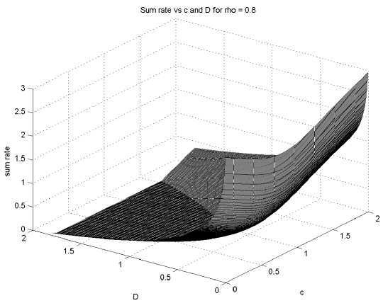
Figure 5: Lattice based scheme’s sum-rate vs $c$ and distortion $D$ for $\rho=0.8$

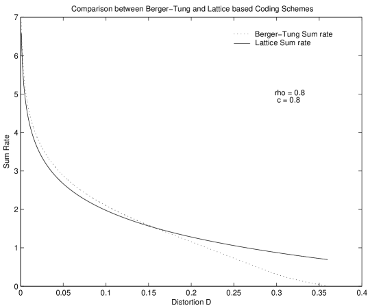
Figure 6: Comparison of the sum-rates of the 2 schemes

We observe that the lattice based scheme performs better than the Berger-Tung based scheme for small distortions provided $\rho$ is sufficiently high and $c$ lies in a certain interval. Fig. 7 is a contour plot that illustrates this in detail. The contour labeled $R$ encloses that region in which the pair $(\rho,c)$ should lie for the lattice binning scheme to achieve a sum rate that is at least $R$ units less than the sum rate of the Berger-Tung scheme for some distortion $D$. Observe that we get improvements only for $c>0$.

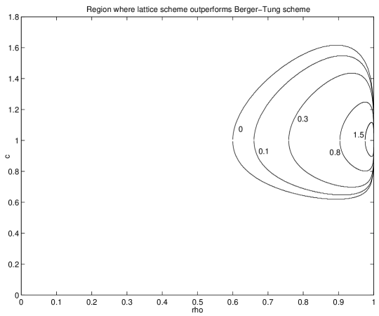
Figure 7: Range of $(\rho,c)$ where the lattice scheme performs better than the Berger Tung scheme

6 Conclusion

We have thus demonstrated a lattice based coding scheme that directly encodes the linear function that the decoder is interested in instead of encoding the sources separately and estimating the function at the decoder. For the case of two users, it is seen that the lattice based coding scheme gives a lower sum-rate for certain values of $\rho,c,D$. Hence, using a combination of the lattice based and the Berger-Tung based coding schemes results in a better rate-region than using any one scheme alone. For the case of reconstructing a linear function of $K$ sources, we have extended this concept to provide an inner bound to the optimal rate-distortion function. Some parts of the inner bound are achieved using a coding scheme that has the following structure: lattice vector quantization followed by “correlated” lattice-structured binning.

Appendix A Derivation of Berger-Tung based scheme’s sum rate

In this section, we derive the sum-rate of the Berger-Tung based scheme given in equations (21)-(23). The sum-rate of the Berger-Tung based coding scheme is given by

$$R_{1}+R_{2} \geq\frac{1}{2}\log\frac{(1+q_{1})(1+q_{2})-\rho^{2}}{q_{1}q_{2}}$$ (113)

where $(q_{1},q_{2})\in\mathbb{R}^{2}_{+}$ should satisfy the distortion constraint

$$D \geq\frac{q_{1}\alpha+q_{2}c^{2}\alpha+q_{1}q_{2}\sigma_{Z}^{2}}{(1+q_{1})(1+q_{2})-\rho^{2}}$$ (114)

where $\mathbb{R}_{+}$ is the set of positive reals and $\alpha=1-\rho^{2}$.

To minimize the sum-rate, we need to minimize the quantity given by equation (113). Using the fact that the log function is monotone and that $(q_{1},q_{2})$ must satisfy the distortion constraint in equation (114), the minimization problem is equivalent to minimizing

$$\frac{(1+q_{1})(1+q_{2})-\rho^{2}}{q_{1}q_{2}} =\frac{q_{1}\alpha+q_{2}c^{2}\alpha+q_{1}q_{2}\sigma_{Z}^{2}}{Dq_{1}q_{2}}$$ (115)

and this is equivalent to minimizing

$$\frac{1}{q_{2}}+\frac{c^{2}}{q_{1}}$$ (116)

subject to the constraint in equation (114).

Assuming that $(q_{1},q_{2})$ satisfy the distortion constraint with equality, one can solve for $q_{2}$ in terms of $q_{1}$ to give

$$q_{2} =\frac{\alpha D-q_{1}(\alpha-D)}{(c^{2}\alpha-D)+q_{1}(\sigma_{Z}^{2}-D)}.$$ (117)

Substituting this in equation (116) gives the function to be minimized as a function of $q_{1}$ alone. The optimal choice of $q_{1}$ is then

$$q_{1}^{*} =\text{argmin }\frac{q_{1}^{2}(\sigma_{Z}^{2}-D)+q_{1}D(c^{2}-1)+\alpha Dc^{2}}{-q_{1}^{2}(\alpha-D)+\alpha Dq_{1}}.$$ (118)

Differentiating with respect to $q_{1}$ and setting the derivative to $0$ gives us a quadratic in $q_{1}$ whose roots are

$$q_{1}^{*} =\frac{\alpha c}{\rho-c}\,\,\text{ or }\,\,\frac{\alpha cD}{2\alpha c-(\rho+c)D}$$ (119)

The second root given above is where the minima occurs. The $q_{2}$ value corresponding to this value of $q_{1}$ is

$$q_{2}^{*} =\frac{\alpha D}{2\alpha c^{2}-(1+\rho c)D}.$$ (120)

Note that these optimal values of $q_{1}$ and $q_{2}$ are positive only for distortions in the range

$$D \leq\min\left\{\frac{2\alpha c}{\rho+c}\,,\,\frac{2\alpha c^{2}}{1+\rho c}\right\}.$$ (121)

For values of $D$ outside this range, the optimal strategy is to let $q_{1}$ or $q_{2}$ go to $\infty$ which effectively means that we encode and transmit only one source.

For $D$ in the range given in equation (121), the sum rate $R_{\text{sum}}=R_{1}+R_{2}$ is found by substituting $q_{1}^{*}$ and $q_{2}^{*}$ in equation (113) to get

$$R_{\text{sum}} \geq\frac{1}{2}\log\frac{4c(\alpha c-\rho D)}{D^{2}}\quad D\leq\min\left\{\frac{2\alpha c}{\rho+c}\,,\,\frac{2\alpha c^{2}}{1+\rho c}\right\}.$$ (122)

For $D$ outside the range given in equation (121), the minimum sum rate is attained by setting either $q_{1}$ or $q_{2}$ as $\infty$. Which quantity goes to $\infty$ depends on which argument of the min function in equation (121) is smaller; equivalently on whether $c>1$ or not. It is easy to see that if $c<1$, $q_{2}=\infty$ and

$$R_{\text{sum}} =\frac{1}{2}\log\frac{(1-\rho c)^{2}}{D-\alpha c^{2}}\quad\text{for }D>\frac{2\alpha c^{2}}{1+\rho c},$$ (123)

and if $c>1$, $q_{1}=\infty$ and

$$R_{\text{sum}} =\frac{1}{2}\log\frac{(c-\rho)^{2}}{D-\alpha}\quad\text{for }D>\frac{2\alpha c}{\rho+c}.$$ (124)

Combining equations (122), (123) and (124) and taking the convex closure of the resulting region, the complete rate region for the Berger-Tung based scheme can be found.

Appendix B Existence of good nested lattices

In this section, we show the existence of nested lattices with any finite degree of nesting such that all the lattice codes involved are simultaneously good source and channel codes. More precisely, we show the existence of a nested lattice $(\Lambda_{1},\dots,\Lambda_{m})$, $\Lambda_{m}\subset\dots\subset\Lambda_{1}$ such that $\Lambda_{i}$, $i=1,\dots,m$ are simultaneously good source and channel codes for sufficiently large lattice dimension $n$.

We use the same nested lattice ensemble as described in [46]. For completeness sake, we include a description of the ensemble.

• Start with a fixed $n$-dimensional lattice $\Lambda_{2}$ which is a good source and channel code. The existence of such a lattice was shown in [47]. Let $G_{\Lambda_{2}}$ be the generator matrix of $\Lambda_{2}$, i.e., $\Lambda_{2}=G_{\Lambda_{2}}\cdot\mathbb{Z}^{n}$.

• Construct a $k\times n$ matrix $G$ whose elements are drawn according to an uniform i.i.d distribution over $\mathbb{Z}_{p}=\{0,1,\dots,p-1\}$ where $p$ is an appropriately chosen prime.

• Define the discrete codebook $\mathcal{C}=\{x\in\mathbb{Z}_{p}^{n}\colon x=y\cdot G\text{ for some }y\in\mathbb{Z}_{p}^{k}\}$.

• Apply Loeliger’s type A construction [52] to form the lattice $\Lambda_{1}^{{}^{\prime}}=p^{-1}\mathcal{C}+\mathbb{Z}^{n}$.

• Transform $\Lambda_{1}^{{}^{\prime}}$ to get the fine lattice $\Lambda_{1}\triangleq G_{\Lambda_{2}}\cdot\Lambda_{1}^{{}^{\prime}}$.

• This construction of $\Lambda_{1}$ can be viewed equivalently as follows. From the lattice $p^{-1}\Lambda_{2}$, pick $k<n$ points at random along with all their multiples modulo-$\Lambda_{2}$. The resulting set of points constitute the fine lattice $\Lambda_{1}$.

By construction, it follows that $\Lambda_{2}\subset\Lambda_{1}$ with the nesting ratio $\sqrt[n]{p^{k}}$. It was shown in [46] that, with high probability, this construction will result in $\Lambda_{1}$ being a good channel code. In [53], it was shown that a nested lattice from this ensemble is, with high probability, a good source code as well. By union bound, it then follows that $\Lambda_{1}$ is simultaneously a good source and channel code with high probability. It follows that there exists nested lattices $(\Lambda_{1},\Lambda_{2})$ such that $\Lambda_{2}\subset\Lambda_{1}$ and both $\Lambda_{1}$ and $\Lambda_{2}$ are simultaneously good source and channel codes.

By iterating this process (with $\Lambda_{1}$ playing the role of $\Lambda_{2}$ in the construction above), one can obtain a nested lattice code with any finite level of nesting. More precisely, for any $m>0$, one can show the existence of a nested lattice $(\Lambda_{1},\dots,\Lambda_{m}),\,\Lambda_{m}\subset\dots\subset\Lambda_{1}$ such that all the lattices $\Lambda_{i},i=1,\dots,m$ are simultaneously good source and channel codes. Moreover, this can be accomplished for any choice of nesting ratios.

Appendix C Proof of convergence to Gaussianity of $e_{q}$

In this section, we prove the claim that $e_{q}=e_{q_{1}}-e_{q_{2}}$ tends to a white Gaussian noise in the Kullback-Leibler divergence sense. Note that $e_{q_{1}}$ and $e_{q_{2}}$ are independent.

We use the following properties of subtractive dither quantization noise and the associated optimal lattice quantizers [42].

• The subtractive dither quantization noise $e_{q_{i}}$ is uniformly distributed over the basic Voronoi region $\mathcal{V}_{0,{1i}}$ of the fine lattice $\Lambda_{1i}$ for $i=1,2$. It follows from equation (5) that

  $$\mathbb{E}\parallel e_{q_{i}}\parallel^{2}=n\sigma^{2}(\Lambda_{1i})\quad\text{for }i=1,2.$$ (125)

• For optimal lattice quantizers, the components of $e_{q_{i}},i=1,2$ are uncorrelated and have the same power,i.e., their correlation matrices $\Sigma_{e_{q_{i}}}$ can be written as

  $$\Sigma_{e_{q_{i}}}=\sigma^{2}(\Lambda_{1i})\mathbf{I}_{n\times n}\quad\text{for }i=1,2.$$ (126)

• For optimal lattice quantizers, as the lattice dimension $n\rightarrow\infty$, the distribution of $e_{q_{i}},i=1,2$ tends to a white Gaussian vector of same covariance in the Kullback-Leibler divergence sense. Taking into account equation (125), this can be written as

  $$\frac{1}{n}D\left(e_{q_{i}}\parallel\mathcal{N}(0,\sigma^{2}(\Lambda_{1i})\mathbf{I}_{n\times n})\right)\rightarrow 0\quad\text{for }i=1,2$$ (127)

  in terms of the Kullback-Leibler divergence $D(.\parallel.)$ or equivalently,

  $$h(e_{q_{i}})\rightarrow\frac{n}{2}\log 2\pi e\sigma^{2}(\Lambda_{1i})\quad\text{for }i=1,2$$ (128)

  in terms of differential entropy $h(\cdot)$.

To show the convergence of $e_{q}$ to a white Gaussian random vector, we use the entropy power inequality and the fact that for a given covariance matrix, the Gaussian distribution maximizes differential entropy.

The entropy power inequality [13] states that for two independent $n$-dimensional random vectors $X$ and $Y$ (having densities),

$$2^{\frac{2}{n}h(X+Y)} \geq 2^{\frac{2}{n}h(X)}+2^{\frac{2}{n}h(Y)}.$$ (129)

This inequality applied to the subtractive dither quantization noises gives

$$2^{\frac{2}{n}h(e_{q_{1}}-e_{q_{2}})} \geq 2^{\frac{2}{n}h(e_{q_{1}})}+2^{\frac{2}{n}h(e_{q_{2}})}.$$ (130)

As $n\rightarrow\infty$, by equation (128), the right hand side of equation (130) tends to $2\pi e(\sigma^{2}(\Lambda_{11})+\sigma^{2}(\Lambda_{12}))$. So, we have the following lower bound on the limit of the differential entropy of $e_{q}$.

$$\lim_{n\rightarrow\infty}h(e_{q}) \geq\frac{n}{2}\log 2\pi e(\sigma^{2}(\Lambda_{11})+\sigma^{2}(\Lambda_{12})).$$ (131)

To prove the inequality in the other direction, note that equation (126) implies that the covariance matrix of $e_{q}$ is $(\sigma^{2}(\Lambda_{11})+\sigma^{2}(\Lambda_{12}))\mathbf{I}_{n\times n}$. Since the Gaussian distribution maximizes differential entropy for a given covariance matrix, we have

$$h(e_{q}) \leq\frac{n}{2}\log 2\pi e(\sigma^{2}(\Lambda_{11})+\sigma^{2}(\Lambda_{12}))$$ (132)

Combining equations (131) and (132), we have the desired result that (if optimal lattice quantizers are used)

$$\lim_{n\rightarrow\infty}h(e_{q}) =\frac{n}{2}\log 2\pi e(\sigma^{2}(\Lambda_{11})+\sigma^{2}(\Lambda_{12})).$$ (133)

In words, $e_{q}$ tends in the Kullback-Leibler divergence sense to a white Gaussian random vector with covariance matrix $(\sigma^{2}(\Lambda_{11})+\sigma^{2}(\Lambda_{12}))\mathbf{I}_{n\times n}$.

Appendix D Derivation of optimal Lattice parameters

In the coding schemes of both Section 3 and Section 4, we scale the sources before encoding them. Here, we briefly outline a justification for the specific scaling constants used. We restrict ourselves to the case where all the $K$ users encode their sources using lattice binning. In the notation of Section 4.2, this corresponds to $\Theta=\{1,\ldots,K\}$.

Let the function to be reconstructed be $Z=\sum_{i=1}^{K}c_{i}X_{i}=cX^{n}$. Here $c$ is a row vector with its $i$th component as $c_{i}$ and $X^{n}$ is a column vector of the sources $X_{i}$. $\Sigma$ is the covaraince matrix of the random vector $X^{n}$. Let the $i$th encoder scale its input by an arbitrary constant $\eta_{i}$. Let $\eta\triangleq[\eta_{1},\ldots,\eta_{K}]$. Choose a tuple $\mathcal{Q}=(q_{1},\ldots,q_{K})\in\mathbb{R}_{+}^{K}$ just as in Section 4.4.2.

It can be shown from analysis similar to the ones in Section 3.2 and 4.2 that the decoder can, with high probability, reconstruct the function $\eta X^{n}+Q$ where $Q$ approaches a white Gaussian noise of variance $q=\sum_{i=1}^{K}q_{i}$. From equation (64), it follows that the function $f$ used for decoding is

$$\hat{Z} =\left(\frac{c\Sigma\eta^{T}}{\eta\Sigma\eta^{T}+q}\right)(\eta X^{n}+Q)$$ (134)

and the corresponding distortion is

$$D =\sigma_{Z}^{2}-\frac{(c\Sigma\eta^{T})^{2}}{\eta\Sigma\eta^{T}+q}.$$ (135)

This fixes the value of $q$. The second moment of the channel code used is $\sigma^{2}(\Lambda_{2})=\text{Var}(\sum_{i}\eta_{i}X_{i}+q_{i})=\eta\Sigma\eta^{T}+q$. This gives us the rate tuple

$$R_{i} =\frac{1}{2}\log\frac{\eta\Sigma\eta^{T}+q}{q_{i}}\quad\text{for }i=1,\ldots,K$$ (136)

Eliminating $q_{i}$ using $q=\sum_{i}q_{i}$ gives us the rate region

$$\sum_{i=1}^{K}2^{-2R_{i}} \leq 1-(\sigma_{Z}^{2}-D)\frac{\eta\Sigma\eta^{T}}{(c\Sigma\eta^{T})^{2}}.$$ (137)

This rate region is largest when the RHS is maximum. Maximizing the RHS as a function of $\eta$ results in $\eta=\xi\cdot c$ as the only solution for some constant $\xi$. However, all constants $\xi$ result in the same rate region.

References

- [1] D. Slepian and J. K. Wolf, “A coding theorem for multiple access channels with correlated sources,” Bell Syst. Tech. J., vol. 52, pp. 1037–1076, September 1973.
- [2] A. D. Wyner, “Recent results in Shannon theory,” IEEE Trans. on Inform. Theory, vol. 20, pp. 2–10, January 1974.
- [3] A. D. Wyner, “On source coding with side information at the decoder,” IEEE Trans. on Inform. Theory, vol. IT-21, pp. 294–300, May 1975.
- [4] R. Ahlswede and J. Korner, “Source coding with side information and a converse for degraded broadcast channels,” IEEE Trans. Inform. Theory, vol. IT- 21, pp. 629–637, November 1975.
- [5] A. D. Wyner and J. Ziv, “The rate-distortion function for source coding with side information at the decoder,” IEEE Trans. Inform. Theory, vol. IT- 22, pp. 1–10, January 1976.
- [6] T. Berger, “Multiterminal source coding,” in Lectures presented at CISM summer school on the Inform. Theory approach to communications, July 1977.
- [7] S.-Y. Tung, Multiterminal source coding. PhD thesis, School of Electrical Engineering, Cornell University, Ithaca, NY, May 1978.
- [8] T. Berger, K. B. Housewright, J. K. Omura, S. Tung, and J. Wolfowitz, “An upper bound on the rate distortion function for source coding with partial side information at the decoder,” IEEE Trans. Inform. Theory, vol. IT- 25, pp. 664–666, November 1979.
- [9] S. Gelfand and M. Pinsker, “Coding of sources on the basis of observations with incomplete information,” Problemy Peredachi Informatsii, vol. 15, pp. 45–57, Apr-June 1979.
- [10] J. Korner and K. Marton, “How to encode the modulo-two sum of binary sources,” IEEE Trans. Inform. Theory, vol. IT-25, pp. 219–221, March 1979.
- [11] T. S. Han, “Source coding with cross observations at the encoders,” IEEE Trans. Inform. Theory, vol. IT-25, pp. 360–361, May 1979.
- [12] I. Csiszár and J. Korner, Information Theory: Coding Theorems for Discrete Memoryless Systems. Academic Press Inc. Ltd., 1981.
- [13] T. M. Cover and J. A. Thomas, Elements of Information Theory. New York:Wiley, 1991.
- [14] T. S. Han and K. Kobayashi, “A dichotomy of functions F(X,Y) of correlated sources (X,Y),” IEEE Trans. on Inform. Theory, vol. 33, pp. 69–76, January 1987.
- [15] R. Ahlswede and T. S. Han, “On source coding with side information via a multiple-access channel and related problems in multi-user information theory,” IEEE Trans. on Inform. Theory, vol. 29, pp. 396–412, May 1983.
- [16] R. W. Yeung and T. Berger, “Multiterminal source coding with one distortion criterion,” IEEE Trans. on Inform. Theory, vol. 35, pp. 228–236, March 1989.
- [17] H. Viswanathan, Z. Zhang, and T. Berger, “The CEO problem,” IEEE Trans. on Inform. Theory, vol. 42, pp. 887–902, May 1996.
- [18] H. Viswanathan and T. Berger, “The quadratic Gaussian CEO problem,” IEEE Trans. on Inform. Theory, vol. 43, pp. 1549–1559, September 1997.
- [19] P. Viswanath, “Sumrate of multiterminal Gaussian source coding ,” in DIMACS workshop on Network Information Theory, (Piscataway, NJ), April 2002.
- [20] H. Yamamoto and K. Itoh, “Source coding theory for multiterminal communication systems with a remote source,” The Transactions of the IECE of Japan, vol. E-63, pp. 700–706, October 1980.
- [21] T. J. Flynn and R. M. Gray, “Encoding of correlated observations,” IEEE Trans. Inform. Theory, vol. IT-33, pp. 773–787, November 1987.
- [22] R. Dobrushin and B. Tsybakov, “Information transmission with additional noise,” IRE Trans. Inform. Theory, vol. IT- 18, pp. S293–S304, 1962.
- [23] H. S. Witsenhausen, “Indirect rate distortion problems,” IEEE Trans. Inform. Theory, vol. IT- 26, pp. 518–521, September 1980.
- [24] Y. Oohama, “Gaussian multiterminal source coding,” IEEE Trans. Inform. Theory, vol. IT- 43, pp. 1912–1923, November 1997.
- [25] Y. Oohama, “The rate-distortion function for the quadratic Gaussian CEO problem,” IEEE Trans. Inform. Theory, vol. IT-44, pp. 1057–1070, May 1998.
- [26] Y. Oohama, “Rate-distortion theory for Gaussian multiterminal source coding systems with several side informations at the decoder,” IEEE Trans. Inform. Theory, vol. IT-51, pp. 2577–2593, July 2005.
- [27] Y. Oohama, “Rate distortion region for separate coding of correlated Gaussian remote observations,” in Allerton Conference, (Monticello, IL), September 2005.
- [28] Y. Oohama, “Separate source coding of correlated Gaussian remote sources,” in Workshop on Information theory and Applications (ITA), (San Diego, CA), January 2006.
- [29] A. B. Wagner and V. Anantharam, “An improved outer bound for the multiterminal source-coding problem,” in IEEE International Symposium on Information Theory (ISIT ’05), (Adelaide, Australia), September 2005.
- [30] V. Prabhakaran, K. Ramchandran, and D. Tse, “Rate region of the quadratic Gaussian CEO problem,” in IEEE International Symposium on Information Theory (ISIT ’04), (Chicago, IL), p. 117, June 2004.
- [31] A. Orlitsky and J. R. Roche, “Coding for computing,” IEEE Trans. Inform. Theory, vol. IT-47, pp. 903–917, March 2001.
- [32] H. Yamamoto, “Wyner-Ziv theory for a general function of the correlated sources,” IEEE Trans. Inform. Theory, vol. IT-28, pp. 803–807, September 1982.
- [33] H. Feng, M. Effros, and S. A. Savari, “Functional source coding for networks with receiver side information,” in Proc. of the 42nd annual Allerton conference on Communication, Control and Computing, (Monticello, IL), September 2004.
- [34] M. Gastpar, “The Wyner-Ziv problem with multiple sources,” IEEE Trans. Inform. Theory, vol. IT-50, pp. 2762–2768, November 2004.
- [35] A. B. Wagner, S. Tavildar, and P. Viswanath, “The rate-region of the quadratic Gaussian two-terminal source-coding problem,” arXiv:cs.IT/0510095.
- [36] S. Tavildar, P. Viswanath, and A. B. Wagner, “The Gaussian many-help-one distributed source coding problem,” in Proc. of the 2006 IEEE Inform. Theory Workshop (ITW ’06), (Chengdu, China), pp. 596–600, October 2006.
- [37] S. Jana and R. Blahut, “Achievable region for multiterminal source coding with lossless decoding in all sources except one,” to appear in IEEE Inform. Theory Workshop (ITW ’07), (Lake Tahoe, CA), September 2007.
- [38] S. Jana, “Unified theory of source coding: Part I - two terminal problems,” arXiv:cs/0508118v2.
- [39] S. Jana, “Unified theory of source coding: Part II - multiterminal problems,” arXiv:cs/0508119v1
- [40] I. Csiszar, “Linear codes for sources and source networks: Error exponents, universal coding,” IEEE Trans. Inform. Theory, vol. IT- 28, pp. 585–592, July 1982.
- [41] R. Zamir and M. Feder, “On universal quantization by randomized uniform lattice quantizers,” IEEE Trans. Inform. Theory, vol. IT- 38, pp. 428–436, March 1992.
- [42] R. Zamir and M. Feder, “On lattice quantization noise,” IEEE Trans. Inform. Theory, vol. IT-42, pp. 1152–1159, July 1996.
- [43] S. Shamai, S. Verdu, and R. Zamir, “Systematic lossy source/channel coding,” IEEE Trans. on Inform. Theory, vol. 44, pp. 564–579, March 1998.
- [44] R. Zamir and T. Berger, “Multiterminal source coding with high resolution,” IEEE Trans. Inform. Theory, vol. IT-45, pp. 106–117, January 1999.
- [45] R. Zamir, S. Shamai, and U. Erez, “Nested linear/lattice codes for structured multiterminal binning,” IEEE Trans. Inform. Theory, vol. IT-48, pp. 1250–1276, June 2002.
- [46] U. Erez and R. Zamir, “Achieving 1/2 log(1+SNR) on the AWGN channel with lattice encoding and decoding,” IEEE Trans. Inform. Theory, vol. IT- 50, pp. 2293–2314, October 2004.
- [47] U. Erez, S. Litsyn, and R. Zamir, “Lattices which are good for (almost) everything,” IEEE Trans. Inform. Theory, vol. IT- 51, pp. 3401–3416, October 2005.
- [48] H. Minkowski, “Dichteste gitterförmige Lagerung kongruenter Körper,” Nachr. Ges. Wiss. Göttingen, pp. 311–355, 1904.
- [49] E. Hlawka, “Zur Geometrie der Zahlen,” Math.Z., vol. 49, pp. 285–312, 1944.
- [50] R. Kershner, “The number of circles covering a set,” Amer. Jour. Math., vol. 61, pp. 665–671, 1939.
- [51] C. A. Rogers, Packing and Covering. Cambridge University Press, Cambridge, 1964.
- [52] H. A. Loeliger, “Averaging bounds for lattices and linear codes,” IEEE Trans. Inform. Theory, vol. IT- 43, pp. 1767–1773, November 1997.
- [53] D. Krithivasan and S.S. Pradhan, “A proof of the existence of good nested lattices,” http://www.eecs.umich.edu/techreports/systems/cspl/cspl-384.pdf.
- [54] J. H. Conway and N. J. A. Sloane, Sphere Packings, Lattices and Groups. Springer, 1992.
- [55] A. Kirac and P. Vaidyanathan, “Results on lattice vector quantization with dithering,” IEEE Trans. Circuits and Systems II: Analog and Digital Signal Processing, vol. 43, pp. 811–826, December 1996.
- [56] V. A. Vaishampayan, N. J. A. Sloane and S. D. Servetto, “Multiple-description vector quantization with lattice codebooks: design and analysis,” IEEE Trans. Inform. Theory, vol. IT-47, pp. 1718–1734, July 2001.
- [57] Y. Frank-Dayan and R. Zamir, “Dithered lattice-based quantizers for multiple descriptions,” IEEE Trans. Inform. Theory, vol. IT-48, pp. 192–204, January 2002.
- [58] V. K. Goyal, J. A. Kelner and J. Kovacevic, “Multiple description vector quantization with a coarse lattice,” IEEE Trans. Inform. Theory, vol. IT-48, pp. 781–788, March 2002.
- [59] S. N. Diggavi, N. J. A. Sloane and V. A. Vaishampayan, “Asymmetric multiple description lattice vector quantizers,” IEEE Trans. Inform. Theory, vol. IT-48, pp. 174–191, January 2002.
- [60] J. Ostergaard, Multiple-description lattice vector quantization. PhD thesis, Delft University of Technology, Netherlands, June 2007.
- [61] G. Poltyrev, “On coding without restrictions for the AWGN channel,” IEEE Trans. on Inform. Theory, vol. 40, pp. 409–417, March 1994.