Muon Production in Low-Energy
Electron-Nucleon and Electron-Nucleus Scattering

Abstract

Recently, muon production in electron-proton scattering has been suggested as a possible candidate reaction for the identification of lepton-flavor violation due to physics beyond the Standard Model. Here we point out that the Standard-Model processes $e^{-}p\rightarrow\mu^{-}p\bar{\nu}_{\mu}\nu_{e}$ and $e^{-}p\rightarrow e^{-}n\mu^{+}\nu_{\mu}$ can cloud potential beyond-the-Standard-Model signals in $ep$ collisions. We find that Standard-Model $ep\rightarrow\mu X$ cross sections exceed those from lepton-flavor-violating operators by several orders of magnitude. We also discuss the possibility of using a nuclear target to enhance the $ep\rightarrow\mu X$ signal.

I Introduction

A number of experiments over the past decade provide compelling evidence that the neutrino mass matrix is non-diagonal in the basis of weak eigenstates $|\nu_{\alpha}\rangle;\alpha=e,\mu,~{}{\rm and}~{}\tau$ (see Fogli for a recent review). This knowledge has led to renewed interest in lepton-flavor violation (LFV), which can be probed by searches for rare decays such as $\mu\rightarrow e\gamma$. Such LFV decays are possible when the Standard Model is extended to include neutrino mass and neutrino mixing, but the resulting cross section is exceedingly small (branching ratio, ${\rm BR}\sim 10^{-60}$) as the process scales with the fourth power of the ratio of the neutrino mass to the $W$-boson mass Diener:2004kq . However, a significantly larger branching ratio, ${\rm BR}\sim 10^{-12}$, results from the Minimal Super-Symmetric extension of the Standard Model (MSSM) Blazek:2004cg . The MEG (mu$\rightarrow$e gamma) experiment at the Paul Scherer Institute (PSI) Ritt:2006cg is capable of detecting branching ratios as small as $10^{-13}$ at a 90% confidence level, and will search for the LFV decay $\mu\rightarrow e\gamma$. Such searches for lepton-flavor violation potentially offer an intriguing window on beyond-the-Standard-Model (BSM) physics.

Recently, the possibility of observing lepton-flavor violation in fixed-target electron scattering has been raised as an alternative Diener:2004kq to experiments searching for the rare $\mu\rightarrow e\gamma$ decay. Facilities with electron beams of high intensity and significant duty factor, such as Jefferson Lab, seem to be natural places to perform experiments to search for $ep\rightarrow\mu p$. Hereafter, we will refer to this electron-to-muon conversion process as EMU. However, the conclusion of Ref. Diener:2004kq is that even under the most favorable dynamical scenario (a heavy right-handed Majorana neutrino with $m_{\nu}\sim{\cal O}(m_{W}))$, the Standard-Model supplemented by dynamics that results in neutrino oscillations yields a cross section $\sigma\approx 10^{-27}$ femtobarns (fb) for EMU—so low as to be inaccessible to current experiments.

In this paper, we discuss two Standard-Model processes that can cloud an EMU signal in $e^{-}p$ scattering by generating final states $\mu^{-}X$ other than the desired final state $\mu^{-}p$. In Standard-Model mechanisms, the additional particles $X$ must have baryon number 1, muon lepton number –1, and electron lepton number +1. Two such reactions are: (i) $e^{-}p\rightarrow\mu^{-}\bar{\nu}_{\mu}\nu_{e}p$, and (ii) $e^{-}p\rightarrow e^{-}n\mu^{+}\nu_{\mu}$. From now on, we refer to these reactions as “muon-production processes” in order to distinguish them from EMU.

The first reaction involves only electroweak interactions, and takes place as the electron goes off-shell in the scattering event by an amount corresponding to the momentum of the virtual photon exchanged with the target. The electron then decays via the weak interaction to a muon, accompanied by the emission of $\nu_{e}$ and $\overline{\nu}_{\mu}$. We note that this process can also take place off a neutron, although in practice this implies a nuclear target. In fact, for the nuclear-target case coherent electron interactions with the total nuclear charge can enhance the signal.

The second muon-production process involves the strong interaction. Even when the electron energy is below the pion-production threshold the exchanged virtual photon can interact with the “cloud” of virtual pions that surrounds the nucleon. This can generate an off-shell $\pi^{+}$, which decays to a $\mu^{+}$ and $\nu_{\mu}$. (In electron-nucleus scattering, the presence of neutrons allows $e^{-}n\rightarrow e^{-}p\mu^{-}\bar{\nu}_{\mu}$ to occur through virtual $\pi^{-}$’s.) As the energy of the incident electron approaches the pion threshold, the time for which the virtual pion lives (and hence the distance it travels before decaying) increases. Consequently, these muon-production reactions switch over to pion electro-production at electron energies of about 140 MeV swamping any possible EMU signals.

This paper is organized as follows. Section II presents a pedagogical calculation of electron-proton scattering as a probe of BSM physics using generic low-energy effective couplings that can cause EMU. The diagram involving photon exchange plays a dominant role, but is severely constrained by the experimental bound on the coupling obtained from the $\mu\to e\gamma$ process. (For a specific realization in the MSSM see Ref. Blazek:2004cg .) In Sec. III, we derive the matrix element for the process $e^{-}p\rightarrow\mu^{-}\bar{\nu}_{\mu}\nu_{e}p$ from electroweak theory, compute the size of the cross section, and provide a simple explanation for the order-of-magnitude of our result. In Sec. IV, the virtual-pion production and decay contributions to the matrix element for $ep\rightarrow en\mu^{+}\nu_{\mu}$, and the resulting differential cross section are presented. Due to differences in the interaction couplings and phase-space factors, the cross section for $e^{-}p\rightarrow e^{-}n\mu^{+}\nu_{\mu}$ turns out to be several orders of magnitude larger than that for $e^{-}p\rightarrow\mu^{-}\bar{\nu}_{\mu}\nu_{e}p$. Therefore any EMU experiment seeking BSM (or even electroweak) physics would either have to veto processes in which a scattered electron is detected in coincidence with the produced muon, or, more feasibly, detect the charge of any muons produced in the electron-proton collision. In Sec. V, we describe muon-production in electron-nucleus scattering, including the relative importance of collective nuclear excitations. We present our summary and conclusions in Sec. VI. Details of phase-space integrations and numerics are provided in the appendices.

II Electron-muon conversion via physics beyond the standard model

In this section, we consider the differential cross section for the reaction $ep\rightarrow\mu p$ induced by operators which change lepton flavor, and hence are low-energy manifestations of physics “beyond the Standard Model” (BSM). All such operators are, by definition, dimension five or above, and so they produce cross sections suppressed by (at least) one power of $m_{\mu}/\Lambda$, where $\Lambda$ is the scale of the physics that results in lepton-flavor violation. We will show that there is a dimension-five operator that could, in principle, produce a sizeable $ep\rightarrow\mu p$ cross section. However, in practice, bounds from the non-observation of the process $\mu\rightarrow e\gamma$ preclude any observable muon production via this dimension-five BSM operator.

Figure 1: Beyond-the-Standard-Model contribution to muon production (“electron-muon conversion”). The hatched vertex represents the dimension-five coupling of Eq. (1). The solid lines denote leptons, while the double line is the proton. The particle momenta are indicated in parentheses.

The BSM operator associated with the decay $\mu\rightarrow e\gamma$ can be written as

$${\cal L}_{I}=-\frac{ev}{\Lambda^{2}}(\bar{\psi}_{e}\sigma_{\alpha\beta}F^{\alpha\beta}\psi_{\mu}+\rm{h.c.})\,,$$ (1)

where $\psi_{l}$ is the lepton field of family $l$ ($e~{}{\rm or}~{}\mu$), and $F^{\alpha\beta}$ is the electromagnetic field-strength tensor. The object $v$ is the Higgs vacuum expectation value, and $\Lambda$ is the scale of the BSM physics that induces this operator. The Higgs vacuum expectation value appears because while the operator is of dimension five, it is suppressed by an additional power of $v/\Lambda$ because it changes lepton chirality. Dimension-six BSM structures which have the low-energy form

$${\cal L}_{I}^{\rm contact}\sim\frac{e}{\Lambda^{2}}\bar{\psi}_{e}O\psi_{\mu}\bar{N}ON\,,$$ (2)

where $N$ denotes the nucleon field and the $O$’s are operators (potentially with Lorentz indices that are contracted with one another) can also appear in ${\cal L}_{I}$. However, their effects are suppressed relative to the operator in Eq. (1).

The Feynman diagram for $ep\rightarrow\mu p$ for the coupling in Eq. (1) is shown in Fig. 1. The general form of the nucleon current (given parity invariance, time-reversal invariance and gauge invariance) can be parameterized using two functions $F_{1}$ and $F_{2}$:

$$\langle j^{\mu}\rangle=e\bar{u}_{N}({\bf p}^{\prime})\left[F_{1}(Q^{2})\gamma^{\mu}+\kappa F_{2}(Q^{2})\frac{i}{2M}\sigma^{\mu\nu}q_{\nu}\right]u_{N}({\bf p})\,,$$ (3)

where $F_{1}(Q^{2})$ and $F_{2}(Q^{2})$ are the Dirac and Pauli nucleon form factors respectively, $\kappa$ is the proton’s anomalous magnetic moment, $M$ is the proton mass, and $q=p^{\prime}-p$, with $Q^{2}=-q^{2}>0$. Employing this to evaluate the matrix element associated with the diagram in Fig. 1, we find

$${\cal M}=\frac{e^{2}v}{\Lambda^{2}}\frac{1}{-q^{2}}\bar{u}_{\mu}({\bf p}_{2}^{\prime})[\gamma_{\alpha},\not\!q]u_{e}({\bf p}_{2})\bar{u}_{N}({\bf p}^{\prime})\left[F_{1}(Q^{2})\gamma^{\alpha}+\kappa\frac{F_{2}(Q^{2})}{4M}[\gamma^{\alpha},\not\!q]\right]u_{N}({\bf p})\,,$$ (4)

where now $q=p_{2}^{\prime}-p_{2}=p-p^{\prime}$ is the four-momentum of the virtual photon that is exchanged.

The spin-summed-and-averaged squared matrix element can be written as

$$\overline{|{\cal M}|^{2}}=\frac{e^{4}v^{2}}{\Lambda^{4}}L^{\alpha\beta}H_{\alpha\beta}\frac{1}{(q^{2})^{2}}\,,$$ (5)

where the lepton and hadron tensors are both transverse with respect to the photon four-vector $q$, that is,

$$q^{\alpha}H_{\alpha\beta}=q^{\beta}H_{\alpha\beta}=q^{\alpha}L_{\alpha\beta}=q^{\beta}L_{\alpha\beta}=0\,.$$ (6)

The lepton tensor can thus be replaced by

$$\tilde{L}_{\alpha\beta}={\rm Tr}(\not\!p_{2}^{\prime}\gamma_{\alpha}\not\!q\not\!p_{2}\not\!q\gamma_{\beta})\,,$$ (7)

where terms proportional to the electron mass have been neglected, as they are suppressed by $m_{e}/m_{\mu}$. Straightforward evaluation then yields

$$\tilde{L}_{\alpha\beta}=-4q^{2}({p_{2}^{\prime}}_{\alpha}{p_{2}}_{\beta}+{p_{2}}_{\alpha}{p_{2}^{\prime}}_{\beta}-p_{2}^{\prime}\cdot p_{2}g_{\alpha\beta})-8p_{2}^{\prime}\cdot qp_{2}\cdot qg_{\alpha\beta}\,.$$ (8)

The evaluation of $\overline{|{\cal M}|^{2}}$ reveals that effects due to the Pauli form factor $F_{2}$ are suppressed by $Q^{2}/4M^{2}$. Below pion-production threshold this parameter is at most 0.02, and so in what follows we neglect the contribution to $H^{\alpha\beta}$ from the nucleon Lorentz structure $i\sigma^{\mu\nu}q_{\nu}$. For the proton,

$$F_{1}(Q^{2})=1-\frac{1}{6}\langle r_{p}^{2}\rangle Q^{2}+{\cal O}(Q^{4}),$$ (9)

with $\langle r_{p}^{2}\rangle^{1/2}=0.895(18)~{}{\rm fm}$ Sick03 , and so $F_{1}(Q^{2})=1$ up to a few per cent correction at the kinematics of interest here. Under these approximations, we obtain

$$H^{\alpha\beta} = {\rm Tr}((\not\!p^{\prime}+M)\gamma^{\alpha}(\not\!p+M)\gamma^{\beta})$$ (10)

$$= 4({p^{\prime}}^{\alpha}p^{\beta}+{p}^{\prime\beta}p^{\alpha}+(M^{2}-p^{\prime}\cdot p)g^{\alpha\beta})\,.$$ (11)

Contraction of the tensors $H$ and $L$ then yields

$$\overline{|{\cal M}|^{2}} = \frac{16e^{4}v^{2}}{\Lambda^{4}}\frac{1}{(Q^{2})^{2}}\{Q^{2}[2(p_{2}^{\prime}\cdot p^{\prime})(p_{2}\cdot p)+2(p_{2}^{\prime}\cdot p)(p^{\prime}\cdot p_{2})-2M^{2}(p_{2}^{\prime}\cdot p_{2})]$$ (12)

$$-4(p_{2}^{\prime}\cdot q)(p_{2}\cdot q)(p^{\prime}\cdot p)-8M^{2}(p_{2}^{\prime}\cdot q)(p_{2}\cdot q)+8(p^{\prime}\cdot p)(p_{2}\cdot q)(p_{2}^{\prime}\cdot q)\}\,.$$

Dropping terms which are suppressed by at least one power of $Q^{2}/M^{2}$ relative to the dominant contribution, we are left with

$$\overline{|{\cal M}|^{2}}=\frac{16e^{4}v^{2}}{\Lambda^{4}}\frac{1}{(Q^{2})^{2}}\left[(Q^{2})(s-M^{2}-m_{\mu}^{2}-Q^{2})(s-M^{2})-M^{2}(m_{\mu}^{2}+Q^{2})m_{\mu}^{2}+O(Q^{6})\right]\,,$$ (13)

where $s=(p+p_{2})^{2}$.

Working now in the lab frame, and neglecting nucleon recoil, we have

$$E_{\mu} = E_{e};$$ (14)

$$q^{2} \equiv -Q^{2}=m_{\mu}^{2}-2E_{e}^{2}+2E_{e}\sqrt{E_{e}^{2}-m_{\mu}^{2}}\cos\theta_{\mu}\,,$$ (15)

where $\theta_{\mu}$ is the angle between the outgoing muon and the incoming electron beam. The differential cross section is then

$$\frac{d\sigma}{d\Omega_{\mu}}=\frac{4\alpha^{2}v^{2}}{\Lambda^{4}}\sqrt{\bar{E_{e}}^{2}-1}~{}~{}f(\bar{E_{e}},\cos\theta_{\mu})\,,$$ (16)

with $\bar{E_{e}}=E_{e}/m_{\mu}$ and

$$f(\bar{E_{e}},\cos\theta_{\mu})=\frac{8\bar{E_{e}}^{4}-6\bar{E_{e}}^{2}+2\bar{E_{e}}\sqrt{\bar{E_{e}}^{2}-1}(1-4\bar{E_{e}}^{2})\cos\theta_{\mu}}{(2\bar{E_{e}}^{2}-2\sqrt{\bar{E_{e}}^{2}-1}\bar{E_{e}}\cos\theta_{\mu}-1)^{2}}\,.$$ (17)

Integrating this over the muon solid angle $\Omega_{\mu}$, we obtain

$$\sigma=\frac{16\pi\alpha^{2}v^{2}}{\Lambda^{4}}\sqrt{\bar{E_{e}}^{2}-1}\left[2\frac{\sqrt{\bar{E_{e}}^{2}-1}}{\bar{E_{e}}}\ln\left(\frac{\bar{E_{e}}+\sqrt{\bar{E_{e}}^{2}-1}}{\bar{E_{e}}-\sqrt{\bar{E_{e}}^{2}-1}}\right)-1\right]\,.$$ (18)

For $E_{e}$ just below pion threshold, the kinematic factor in the square brackets is about 2. Taking $v\approx 200$ GeV and $\Lambda=1$ TeV results in a predicted cross section on the order of $100$ fb, which would definitely be observable. Including the nucleon-recoil terms neglected in the derivation of Eq. (18) would result in corrections of order $\frac{E_{e}}{M}$, which are potentially as large as 20% or so, but do not change the order-of-magnitude of $\sigma$.

On the other hand, dimension-six BSM operators of the type in Eq. (2) do not induce effects mediated by low-momentum photons. If such operators do not contain additional derivatives they cannot produce powers of the nucleon mass in the numerator, and so the largest cross section they can yield is

$$\sigma\sim\frac{\alpha^{2}m_{\mu}^{2}}{\Lambda^{4}}\,,$$ (19)

which is suppressed by $\left(\frac{m_{\mu}}{v}\right)^{2}\hskip 1.99997pt\raisebox{2.15277pt}{$<$}\raisebox{-3.00003pt}{$\sim$}\hskip 1.99997pt10^{-6}$ compared to the long-range mechanism depicted in Fig. 1. Operators $O$ that contain additional derivatives will be suppressed even further by at least one factor of the small parameter $\frac{M}{\Lambda}$.

The result (18) suggests that electron scattering from a proton target could provide access to BSM physics over a sizeable range of $\Lambda$. However, this prediction does not take into account the constraint on the $\mu\rightarrow e\gamma$ coupling from the non-observance of this muon decay branch. As we shall see, this places stringent limits on the size of the cross section for the process in Fig. 1.

The operator in Eq. (1) produces an amplitude for the rare decay $\mu\rightarrow e\gamma$ that, in the muon rest frame, takes the form

$${\cal M}_{\mu\rightarrow e\gamma}=-\frac{iev}{\Lambda^{2}}\bar{u}_{e}(-{\bf q})[\gamma^{\alpha},\not\!q]u_{\mu}(0)\varepsilon_{\alpha}\,,$$ (20)

where $\varepsilon$ is the photon polarization vector, and $q$ is the photon four-momentum. From this, we obtain

$$\overline{|{\cal M}_{\mu\rightarrow e\gamma}|^{2}}=\frac{2e^{2}v^{2}m_{\mu}^{3}}{\Lambda^{4}}\,.$$ (21)

Converting this to a decay rate, and integrating over final electron states, we find

$$\Gamma_{\mu\rightarrow e\gamma}=\frac{\alpha v^{2}m_{\mu}^{3}}{2\Lambda^{4}}\,.$$ (22)

If we now use the result for the predominant muon decay mode Cheng:1985bj

$$\Gamma_{\mu\rightarrow e\nu_{\mu}\bar{\nu}_{e}}=\frac{G_{F}^{2}m_{\mu}^{5}}{192\pi^{3}}\,,$$ (23)

(here $G_{F}=\frac{e^{2}}{2^{5/2}M_{W}^{2}{\rm sin}^{2}\theta_{W}}$ is the Fermi coupling constant, with $M_{W}=80.41$ GeV the W-boson mass and $\theta_{W}$ the Weinberg angle) we find that the branching ratio for $\mu\rightarrow e\gamma$ is

$${\rm BR}(\mu\rightarrow e\gamma)=96\pi^{3}\alpha\frac{v^{2}}{\Lambda^{4}}\frac{1}{m_{\mu}^{2}G_{F}^{2}}\,.$$ (24)

But the factor $\frac{v^{2}}{\Lambda^{4}}$ which appears here is the same as that in the pre-factor in Eq. (18). Consequently, we can eliminate this factor between Eqs. (18) and (24) to obtain

$$\sigma\approx\frac{\alpha}{3\pi^{2}}(m_{\mu}^{2}G_{F})^{2}\frac{1}{m_{\mu}^{2}}{\rm BR}(\mu\rightarrow e\gamma)\,.$$ (25)

Using ${\rm BR}(\mu\rightarrow e\gamma)<4.9\times 10^{-11}$ Yao:2006px , we see that

$$\sigma<7.0\times 10^{-15}~{}{\rm fb}\,.$$ (26)

This is a model-independent constraint on the contribution to the cross section for $ep\rightarrow\mu p$ from photon exchange. Interpreted as a bound on $\Lambda$, we find $\Lambda\geq 1.5\times 10^{4}$ TeV. A similar bound on $\sigma$ was derived within the context of a MSSM calculation of the electron-nucleus to muon-nucleus cross section and ${\rm BR}(\mu\rightarrow e\gamma)$ in Ref. Blazek:2004cg . However, that number was seven orders of magnitude larger than the result of Eq. (26). Part of the difference arises from Ref. Blazek:2004cg ’s consideration of a target with $Z=70$.

One might ask why the apparent scale $\Lambda$ in Eq. (1) is so large—or, equivalently, why the coupling is “unnaturally” small. One possible explanation arises in the scenario known as “minimal-flavor violation” Cirigliano:2005ck . There the physics beyond the Standard Model breaks the lepton-number symmetry of the Standard Model in the same fashion in which it is broken by neutrino mixing. This scenario can account for the small branching ratio for $\mu\rightarrow e\gamma$ in a natural way as long as the product of the relevant neutrino mass and the scale of lepton-flavor violation $\Lambda$ is smaller than $v^{2}$.

Regardless of what physics determines ${\rm BR}(\mu\rightarrow e\gamma)$, our calculations show that the bound on this quantity is sufficiently stringent to preclude the observation of any $ep\rightarrow\mu p$ cross section from the diagram of Fig. 1. Indeed, the contribution of the operator in Eq. (1) is constrained so strongly by the non-observation of this muon decay branch that effects from diagrams with short-range operators of the form (2) are worth considering. In particular, if such EMU’s involved a different scale $\tilde{\Lambda}$, with $\tilde{\Lambda}\ll\Lambda$ of Eq. (1), they may produce a larger effect than (26). However, the estimates provided above indicate that for $\tilde{\Lambda}=1$ TeV, contributions from these dimension-six operators to the $ep\rightarrow\mu p$ cross section would be at most $\sim 10^{-4}$ fb. The conclusion therefore is that beyond-the-Standard-Model physics is unlikely to result in any measurable production of muons when an electron beam impinges on a proton target.

III Muon production via Standard-Model Electroweak Processes

Figure 2: Leading-order Feynman diagram for the process $e^{-}p\rightarrow\mu^{-}\overline{\nu}_{\mu}\nu_{e}p$. Solid lines represent leptons, the double line is a proton, and the dashed line is a $W^{-}$ boson. The four-momentum carried by each external-state particle is indicated in parentheses.

In this section, we evaluate the scattering cross section for the process $e^{-}p\rightarrow\mu^{-}\bar{\nu}_{\mu}\nu_{e}p$. The dominant contribution to the scattering amplitude comes from single-photon exchange given by the Feynman diagram in Fig. 2. Applying the usual QED and Fermi-theory Feynman rules to the upper vertices in the diagram of Fig. 2, and using the single-nucleon current of Eq. (3) for the virtual-photon-nucleon vertex, we get

$$i{\cal M} = \left[-ie\bar{u}_{N}({\bf p}^{\prime})\left\{\gamma^{\mu}F_{1}(Q^{2})+\kappa F_{2}(Q^{2})\frac{i}{2M}\sigma^{\mu\rho}q_{\rho}\right\}u_{N}({\bf p})\right]$$ (27)

$$\times \left(\frac{-ig_{\mu\nu}}{q^{2}}\right)$$

$$\times \frac{G_{F}}{\sqrt{2}}\left[\bar{u}_{\mu}({\bf l}_{2})\gamma^{\alpha}(1-\gamma_{5})v_{\bar{\nu}_{\mu}}({\bf l}_{1})\right]\left[\bar{u}_{e}({\bf p}_{2}^{\prime}-{\bf l})\gamma_{\alpha}(1-\gamma_{5})i\frac{\not\!p_{2}^{\prime}+m_{e}}{{p_{2}^{\prime}}^{2}-m_{e}^{2}}(-ie\gamma^{\nu})u_{e}({\bf p}_{2})\right]\,,$$

For unpolarized electrons, the spin-summed-and-averaged squared matrix element can be expressed as

$$\overline{|{\cal M}|^{2}} = \frac{c_{EW}^{2}(Q^{2})}{2({p_{2}^{\prime}}^{2}-m_{e}^{2})^{2}}H^{\mu\nu}L^{\alpha\beta}W_{\alpha\mu\nu\beta}\,;$$

$$H^{\mu\nu} = {\rm Tr}\left[({\not\!p}^{\prime}+M)\left\{\gamma^{\mu}F_{1}+\frac{\kappa}{2M}i\sigma^{\mu\rho}q_{\rho}F_{2}\right\}(p{\hskip-4.97922pt}/+M)\left\{\gamma^{\nu}F_{1}-\frac{\kappa}{2M}i\sigma^{\nu\theta}q_{\theta}F_{2}\right\}\right]\,,$$

$$L^{\alpha\beta} = {\rm Tr}\left[\not\!l_{2}\gamma^{\alpha}(1-\gamma_{5})\not\!l_{1}\gamma^{\beta}(1-\gamma_{5})\right]\,,$$

$$W_{\alpha\mu\nu\beta} = {\rm Tr}\left[(\not\!p_{2}^{\prime}-l)\gamma_{\alpha}(1-\gamma_{5})(\not\!p_{2}^{\prime}+m_{e})\gamma_{\mu}(\not\!p_{2}+m_{e})\gamma_{\nu}(\not\!p_{2}^{\prime}+m_{e})\gamma_{\beta}(1-\gamma_{5})\right]$$ (28)

with $l\equiv l_{1}+l_{2}$ and

$$c_{EW}^{2}(Q^{2})=\frac{8\pi^{2}\alpha^{2}G_{F}^{2}}{Q^{4}}\,.$$ (29)

The computation of the traces in $W_{\alpha\mu\nu\beta}$ is facilitated by the Chisholm identity

$$\gamma^{\alpha}\gamma^{\beta}\gamma^{\gamma}=g^{\alpha\beta}\gamma^{\gamma}+g^{\beta\gamma}\gamma^{\alpha}-g^{\alpha\gamma}\gamma^{\beta}+i\epsilon^{\alpha\beta\gamma\delta}\gamma_{\delta}\gamma_{5}\,.$$ (30)

Performing the contractions, we obtain

$$\overline{|{\cal M}|^{2}} = \frac{c_{EW}^{2}}{{p_{2}^{\prime}}^{4}}2^{7}\left[\left(p_{2}^{\prime}-l\right)\cdot l_{1}\right]\left\{4F_{1}^{2}(A_{1})-\left(\frac{\kappa}{2M}\right)^{2}F_{2}^{2}(A_{2})-2\kappa F_{1}F_{2}(A_{12})\right\};$$

$$(A_{1}) = 2(p_{2}^{\prime}\cdot l_{2})[(p\cdot p_{2})(p^{\prime}\cdot p_{2}^{\prime})+(p^{\prime}\cdot p_{2})(p\cdot p_{2}^{\prime})-M^{2}(p_{2}\cdot p_{2}^{\prime})]$$

$$-{p_{2}^{\prime}}^{2}[(p\cdot p_{2})(p^{\prime}\cdot l_{2})+(p^{\prime}\cdot p_{2})(p\cdot l_{2})-M^{2}(p_{2}\cdot l_{2})],$$

$$(A_{2}) = 2(p_{2}^{\prime}\cdot l_{2})[2(P\cdot p_{2})(P\cdot p_{2}^{\prime})q^{2}+8M^{2}(q\cdot p_{2})(q\cdot p_{2}^{\prime})+(p_{2}\cdot p_{2}^{\prime})q^{4}]$$

$$-{p_{2}^{\prime}}^{2}[2(P\cdot p_{2})(P\cdot l_{2})q^{2}+8M^{2}(q\cdot p_{2})(q\cdot l_{2})+(p_{2}\cdot l_{2})q^{4}],$$

$$(A_{12}) = 2(p_{2}^{\prime}\cdot l_{2})[2(q\cdot p_{2})(q\cdot p_{2}^{\prime})+q^{2}(p_{2}\cdot p_{2}^{\prime})]-{p_{2}^{\prime}}^{2}[2(q\cdot p_{2})(q\cdot l_{2})+q^{2}(p_{2}\cdot l_{2})]\,,$$ (31)

where $P=(p+p^{\prime})$ and terms of ${\cal O}(m_{e}^{2})$ have been dropped as ${p_{2}^{\prime}}^{2}\gg m_{e}^{2}$. To eliminate the interference terms involving $F_{1}F_{2}$, we reexpress $F_{1}$ and $F_{2}$ through the Sachs form factors RGS64

$$G_{E}=F_{1}+\frac{\kappa q^{2}}{4M^{2}}F_{2}\quad{\rm and}\quad G_{M}=F_{1}+\kappa F_{2}$$ (32)

to get

$$\overline{|{\cal M}|^{2}} = \frac{2^{7}c_{EW}^{2}[(p_{2}^{\prime}-l)\cdot l_{1}]}{{p_{2}^{\prime}}^{2}}\biggl{\{}{\cal T}_{1}-2\frac{{p_{2}^{\prime}}^{2}}{p_{2}^{\prime}\cdot l_{2}}{\cal T}_{2}\biggr{\}}\quad;$$

$${\cal T}_{1} = G_{\tau}\left[P^{2}(p_{2}\cdot l_{2})-2(P\cdot p_{2})(P\cdot l_{2})\right]+G_{M}^{2}\left[2(q\cdot p_{2})(q\cdot l_{2})+(p_{2}\cdot l_{2})q^{2}\right]\,,$$

$${\cal T}_{2} = G_{\tau}\left[P^{2}(p_{2}\cdot p_{2}^{\prime})-2(P\cdot p_{2})(P\cdot p_{2}^{\prime})\right]+G_{M}^{2}\left[2(q\cdot p_{2})(q\cdot p_{2}^{\prime})+(p_{2}\cdot p_{2}^{\prime})q^{2}\right]\,,$$ (33)

where $G_{\tau}=(G_{E}^{2}+\tau G_{M}^{2})/(1+\tau)$ with $\tau=Q^{2}/4M^{2}$.

In the laboratory frame, the differential cross section is given by

$$d\sigma = \frac{1}{4ME_{e}}\int\frac{d^{3}l_{1}}{(2\pi)^{3}2E_{\nu_{\mu}}}\frac{d^{3}l_{2}}{(2\pi)^{3}2E_{\mu^{-}}}\frac{d^{3}p^{\prime}}{(2\pi)^{3}2E_{p^{\prime}}}\frac{d^{3}l_{\nu_{e}}}{(2\pi)^{3}2E_{\nu_{e}}}\overline{|{\cal M}|^{2}}$$ (34)

$$\times(2\pi)^{4}\int d^{4}p_{2}^{\prime}\,\delta^{(4)}(p_{2}+p-p_{2}^{\prime}-p^{\prime})\int d^{4}l\,\delta^{(4)}(l-l_{1}-l_{2})\delta^{(4)}(p_{2}^{\prime}-l-l_{\nu_{e}})\,,$$

where $E_{e}$ is the energy of the incoming electron in the laboratory frame, $l_{\nu_{e}}$ is the electron-neutrino’s 4-momentum and the last two delta functions and integrals have been inserted as unity to simplify calculations. The steps given in Appendix A then allow us to obtain from Eq. (34) an expression for the differential cross section per unit solid angle subtended by the detected muon at fixed beam energy:

$$\frac{d\sigma}{d\Omega_{\mu}} = \frac{\alpha^{2}G_{F}^{2}}{32\pi^{5}M^{3}E_{e}}\int_{m_{\mu}}^{E_{e}}dE_{\mu}\sqrt{E_{\mu}-m_{\mu}^{2}}\int_{q_{0}^{l}}^{q_{0}^{u}}\frac{dq_{0}}{q_{0}^{2}}\sqrt{q_{0}^{2}+2Mq_{0}}\int_{{\rm cos}\theta_{q}^{l}}^{{\rm cos}\theta_{q}^{u}}\,d({\rm cos}\theta_{q})$$ (35)

$$\times \int_{\phi_{q}^{l}}^{\phi_{q}^{u}}d\phi_{q}\,(p_{2}-q-l_{2})^{2}\left[\frac{p_{2}^{\prime}.l_{2}}{{p_{2}^{\prime}}^{4}}{\cal T}_{2}-\frac{1}{2{p_{2}^{\prime}}^{2}}{\cal T}_{1}\right]_{(p_{2}^{\prime}=(p_{2}-q),\,q^{2}=-2Mq_{0})}\,.$$

The limits on the $q_{0}$ integral are determined by the electron beam energy. The lower limit of the integral arises because energy transfer to the proton without any momentum transfer is not possible in elastic scattering: the target recoils. In the limit that the muon is produced at rest (${\bf l}_{2}=0$), an analytic expression for both the upper and lower limit of the $q_{0}$ integration can be obtained. This can guide intuition on the importance of collective excitations when the target is replaced by a heavy nucleus (see Sec. V). We find

$$q_{0}^{\pm} = -\frac{B\mp\sqrt{B^{2}-4AC}}{2A}\,;$$

$$A = 4(E_{e}+M-m_{\mu})^{2}-4E_{e}^{2}\,;\quad C=m_{\mu}^{2}(2E_{e}-m_{\mu})^{2}\,,$$

$$B = 2\left[2(E_{e}+M-m_{\mu})m_{\mu}(2E_{e}-m_{\mu})-4E_{e}^{2}M\right]\,.$$ (36)

Furthermore,

$$q_{0}^{-}\equiv\frac{m_{\mu}^{2}}{2(M-m_{\mu})}\leq E_{e}-E_{\mu}\,,$$ (37)

so that the minimum electron beam energy $E_{e}^{\rm min}$ for muon production is then determined by requiring $q_{0}^{-}=E_{e}^{\rm min}-m_{\mu}$, which yields

$$E_{e}^{\rm min}=\frac{m_{\mu}(2M-m_{\mu})}{2(M-m_{\mu})}=111.6\,{\rm MeV}.$$ (38)

The quantity $q_{0}^{-}$ is thus at least 6 MeV, whereas

$$q_{0}^{+}=\frac{(2E_{e}-m_{\mu})^{2}}{2(2E_{e}-m_{\mu}+M)}$$ (39)

which is always less than $E_{e}-m_{\mu}$. The corresponding $Q^{2}$ ranges from 0.01 GeV² to a maximum of $2Mq_{0}^{+}$. The angle between the electron and muon neutrinos (whose masses are neglected) is constrained to $0\leq\angle({\bf l}_{1},{\bf l}_{\nu_{e}})\leq\pi/2$ by the step-function $\Theta(Q^{2})$. The maximum energy in neutrinos is $E_{\nu}^{\rm max}=E_{e}-q_{0}^{-}-m_{\mu}=E_{e}-E_{e}^{\rm min}$.

It is noteworthy that the differential cross section is independent of the azimuthal angle $\phi_{\mu}$. Dependence on $\phi_{\mu}$ appears explicitly in the matrix element through the dot products $(P\cdot l_{2})$ and $(q\cdot l_{2})$ as well as implicitly in the step function $\Theta\left((k-q-l_{2})^{2}\right)$, but this dependence drops out once the ${\rm d}\phi_{q}$ integration is performed. Only differences of azimuthal angles ($\phi_{q}-\phi_{\mu}$) appear in the ${\rm d}\phi_{q}$ integrand as well as in the limits on this integral, so the integral remains invariant. Therefore experiments to measure this process are characterized by $\theta_{\mu}$ alone, and the $\phi$-independence can be used to increase the total number of counts (thereby decreasing the statistical error) by positioning several detectors in an annulus at the same $\theta_{\mu}$.

The integrals in Eq. (35) were evaluated numerically, details of which are presented in Appendix B. The result for the differential cross section $d\sigma/d\Omega_{\mu}$ as a function of electron beam energy at a fixed value of $\theta_{\mu}=\pi/3$ will be presented in Sec. IV. The corresponding total muon-production cross section rises from $3\times 10^{-16}$ fb at $E_{e}=120$ MeV to $4\times 10^{-13}$ fb at $E_{e}=140$ MeV.

The cross section for the reaction $e^{-}p\rightarrow\mu^{-}p\nu_{e}\bar{\nu}_{\mu}$ is thus much smaller than the low-energy approximation to the Rosenbluth cross section for $ep$ elastic scattering HM :

$$\frac{d\sigma}{d\Omega}\approx\frac{\alpha^{2}F_{1}^{2}}{2E_{e}^{2}}\left[\frac{1}{{\rm sin}^{2}\theta{\rm tan}^{2}\theta}+{\cal O}\left(\frac{E_{e}^{2}}{M^{2}}\right)\right].$$ (40)

At $E_{e}=140$ MeV this is $\sim 10^{7}$ fb for all but forward angles where the Coulomb singularity occurs. Thus, muon production via standard-model electroweak processes is down by 20 orders of magnitude as compared to elastic electron-proton scattering. Much of this suppression comes from the extra factor $G_{F}^{2}l_{\nu_{e}}^{2}(l_{\mu}\cdot l_{\nu_{\mu}})$ (with $l_{x}$ the four-momentum of lepton $x$). Numerically, $G_{F}^{2}\sim 10^{-10}$ GeV^-4, $l_{\nu_{e}}\sim 0.01$ GeV, $l_{\mu}\sim 0.1$ GeV, and $l_{\nu_{\mu}}\sim 0.01$ GeV, and so this factor already implies a suppression of 17 orders of magnitude.

Further suppression occurs due to the lower bound on the virtuality of the exchanged photon, which was explained above, and persists even if the muon is detected at $\theta_{\mu}=0$. The Coulomb divergence that is manifest in Eq. (40) as $\theta\rightarrow 0$ and is associated with $Q^{2}\rightarrow 0$ does not appear in $e^{-}p\rightarrow\mu^{-}p\nu_{e}\bar{\nu}_{\mu}$. The suppression relative to the Rosenbluth cross section is therefore even more severe than is implied by the dimensional analysis in the previous paragraph. The lack of enhancement from the exchanged photon going soft is an important feature of muon production.

The cross section predicted for standard-model electroweak $\mu^{-}$ production at the largest energy considered here, $E_{e}\approx m_{\pi}$, is thus two orders of magnitude larger than the largest BSM cross section predicted by Eq. (26). We limit the indicent electron energy to $E_{e}<m_{\pi}$ as for incident energies larger than the pion mass, strong-interaction processes involving the production of an on-shell pion which then decays to a muon will swamp the purely electroweak diagram of Fig. 2. In the following section, we show that a sub-threshold version of the pion-production process yields muon-production cross sections that are significantly larger than those obtained through the mechanism discussed in this section.

IV Muon production via sub-threshold pion production

In electron-proton collisions, muons can also be generated through processes in which a virtual photon couples to a pion which then decays into a muon and a neutrino (Fig. 3). This is a manifestation of the “pion cloud” of the nucleon, and the processes depicted in Fig. 3 are possible even when the pion in the intermediate state is virtual, i.e. $E_{e}$ is significantly below the pion mass. Whereas only negatively charged muons can be produced in the processes considered thus far, this strong-interaction process yields positively charged muons, together with a neutron in the final state. In this section, we evaluate the differential cross section $\frac{d\sigma}{d\Omega_{\mu}}$ for the reaction: $ep\rightarrow en\mu^{+}\nu_{\mu}$.

Figure 3: Leading-order $\chi$PT contributions to $\mu^{+}$-production in electron-proton scattering. The double line denotes the nucleon, the thin solid lines denote leptons and the dashed lines denote pions. Particle momenta are indicated in parentheses. The numbers in parentheses correspond to the individual amplitudes computed below.

Our calculations are performed using chiral perturbation theory ($\chi$PT), the low-energy effective field theory of QCD. $\chi$PT incorporates QCD’s (broken) $SU(2)_{L}\times SU(2)_{R}$ symmetry as well as the pattern of chiral-symmetry breaking in QCD (for a recent review see Ref. Bernard:2006 ). Reactions involving pions, nucleons, and photons (either real or virtual) can be straightforwardly and systematically evaluated using $\chi$PT, as long as the energies involved are well below the excitation energy of the $\Delta$(1232). Here, we perform a tree-level calculation of the process of interest using the leading-order $\chi$PT Lagrangian. For diagrams (1) to (3) in Fig. 3 our calculation is equivalent to evaluating the amplitude for charged-pion electroproduction at leading order ${\cal O}(e)$. Such a leading-order calculation is known to give a reasonable description of the available data for charged-pion photoproduction near threshold Fearing:1999 .

The leading-order $\chi$PT Lagrangian describing the interactions between pions, photons, and nucleons is given by Donoghue:1992dd

$${\cal L}_{\chi\rm{PT}}={\cal L}_{N\pi}^{(1)}+{\cal L}_{\pi\pi}^{(2)}~{}.$$ (41)

Here ${\cal L}_{\pi\pi}^{(2)}$ denotes the leading-order Goldstone-boson Lagrangian

$${\cal L}_{\pi\pi}=\frac{f_{\pi}^{2}}{4}\mbox{Tr}[D_{\mu}U(D^{\mu}U)^{\dagger}]+\frac{f_{\pi}^{2}}{4}\mbox{Tr}(\chi U^{\dagger}+U\chi^{\dagger})~{},$$ (42)

where to leading order in quark masses the matrix $\chi$ is $m_{\pi}^{2}$ times the identity matrix, and ${\cal L}_{N\pi}^{(1)}$ denotes the lowest-order Lagrangian involving baryons:

$${\cal L}^{(1)}_{\pi N}=\bar{\Psi}\left(iD/-\stackrel{{\scriptstyle\circ}}{{M}}+\frac{\stackrel{{\scriptstyle\circ}}{{g}}_{A}}{2}\gamma^{\mu}\gamma_{5}u_{\mu}\right)\Psi~{}.$$ (43)

In the above equations, the pion fields are collected in the matrix $U=\exp(i\tau\cdot\pi/f_{\pi})$, whereas the fields $u=\exp(i{\mathbf{\tau}}\cdot{\pi}/(2f_{\pi}))$ and $u_{\mu}=i(u^{\dagger}\partial_{\mu}u-u\partial_{\mu}u^{\dagger})$. The quantities $\stackrel{{\scriptstyle\circ}}{{g}}_{A}$ and $\stackrel{{\scriptstyle\circ}}{{M}}$ denote the axial coupling constant and the nucleon mass, respectively, in the chiral limit. The covariant derivative acting on the pion matrix is defined as

$$D_{\mu}U\equiv\partial_{\mu}U-ir_{\mu}U+iUl_{\mu}~{},$$ (44)

where $r_{\mu}$ and $l_{\mu}$ denote the appropriate external fields and external electromagnetic fields $\mathcal{A}_{\mu}$ are coupled to the pion field by setting $r_{\mu}=l_{\mu}=\mathcal{A}_{\mu}$. The (chiral and $U(1)_{\rm em}$) covariant derivative acting on the nucleon field is then

$$D_{\mu}\Psi=\biggl{(}\partial_{\mu}+\frac{1}{2}\bigl{(}u^{\dagger}(\partial_{\mu}-ir_{\mu})u+u(\partial_{\mu}-il_{\mu})u^{\dagger}\bigr{)}-i(r_{\mu}+l_{\mu})\biggr{)}\Psi\,.$$ (45)

As our leading-order computation involves only tree-level diagrams, we can employ the relativistic Lagrangian for nucleon and pion fields without concern about contributions from loop graphs that might violate power counting GasserSainioSvarc . We will therefore use relativistic Feynman rules in what follows. The amplitude corresponding to each of the diagrams contributing to $\mu^{+}$-production at leading order (see Fig. 3) is then

$$\mathcal{M}_{1} = -i\sqrt{2}\,V_{ud}G_{F}f_{\pi}g_{\pi NN}\,e^{2}\frac{1}{(k+q)^{2}-m_{\pi}^{2}}\frac{1}{k^{2}-m_{\pi}^{2}}\frac{1}{q^{2}}$$ (46)

$$\qquad\times\bar{u}_{\nu}({\bf k+q-p_{3}})(k/+q/)(1-\gamma^{5})v_{\mu}({\bf p_{3}})$$

$$\qquad\times\bar{u}_{e}({\bf p_{2}-q})(2k/+q/)u_{e}({\bf p_{2}})$$

$$\qquad\times\bar{u}_{N}({\bf p-k})\gamma^{5}u_{N}({\bf p})~{},$$

$$\mathcal{M}_{2} = -i\sqrt{2}\,V_{ud}G_{F}f_{\pi}g_{\pi NN}\,e^{2}\frac{1}{(k+q)^{2}-m_{\pi}^{2}}\frac{1}{(p+q)^{2}-M^{2}}\frac{1}{q^{2}}$$ (47)

$$\qquad\times\bar{u}_{\nu}({\bf k+q-p_{3}})(k/+q/)(1-\gamma^{5})v_{\mu}({\bf p_{3}})$$

$$\qquad\times\bar{u}_{e}({\bf p_{2}-q})\,\gamma_{\mu}\,u_{e}({\bf p_{2}})$$

$$\qquad\times\bar{u}_{N}({\bf p-k})\gamma^{5}(p/+q/+M)\gamma^{\mu}u_{N}({\bf p})~{},$$

$$\mathcal{M}_{3} = -i\sqrt{2}\,V_{ud}G_{F}f_{\pi}g_{\pi NN}\,e^{2}\frac{1}{2M}\frac{1}{(k+q)^{2}-m_{\pi}^{2}}\frac{1}{q^{2}}$$ (48)

$$\qquad\times\bar{u}_{\nu}({\bf k+q-p_{3}})(k/+q/)(1-\gamma^{5})v_{\mu}({\bf p_{3}})$$

$$\qquad\times\bar{u}_{e}({\bf p_{2}-q})\,\gamma^{\mu}\,u_{e}({\bf p_{2}})$$

$$\qquad\times\bar{u}_{N}({\bf p-k})\,\gamma^{5}\gamma_{\mu}\,u_{N}({\bf p})~{},$$

$$\mathcal{M}_{4} = -i\sqrt{2}\,V_{ud}G_{F}f_{\pi}g_{\pi NN}\,e^{2}\frac{1}{(p_{3}-q)^{2}-m_{\mu}^{2}}\frac{1}{k^{2}-m_{\pi}^{2}}\frac{1}{q^{2}}$$ (49)

$$\qquad\times\bar{u}_{\nu}({\bf k+q-p_{3}})(k/+q/)(1-\gamma^{5})(p_{3}/-q/+m_{\mu})\gamma_{\mu}\,v_{\mu}({\bf p_{3}})$$

$$\qquad\times\bar{u}_{e}({\bf p_{2}-q})\,\gamma^{\mu}\,u_{e}({\bf p_{2}})$$

$$\qquad\times\bar{u}_{N}({\bf p-k})\gamma^{5}u_{N}({\bf p})~{},$$

where $g_{\pi NN}=\frac{Mg_{A}}{f_{\pi}}$ at this order, and we adopt $g_{A}=1.26$, $f_{\pi}=92$ MeV, $M=939$ MeV. Note that the crossed counterpart of diagram (2) is zero if only leading-order couplings are considered, as this process involves a neutron in the final state.

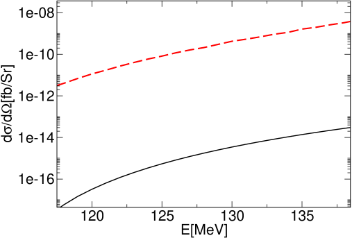
Figure 4: The differential cross section in femtobarns per steradian versus the energy of the incident electron beam. The solid line gives the result for production of a $\mu^{-}$ via the process $e^{-}p\rightarrow\mu^{-}p\bar{\nu}_{\mu}\nu_{e}$ (see Sec. III), and the dashed line is the result for production of a $\mu^{+}$ via the reaction $e^{-}p\rightarrow e^{-}n\mu^{+}\nu_{\mu}$ (see Sec. IV). Both results were evaluated for a representative muon angle $\theta_{\mu}=\pi/3$.

We evaluate the matrix elements ${\cal M}_{1}$–${\cal M}_{4}$ using the package FeynCalc Mertig:1990an . This produces an expression for the spin-averaged-and-summed squared matrix element $\overline{|{\cal M}|^{2}}$ that is lengthy and not particularly illuminating. The differential cross section is then

$$\frac{d\sigma}{d\Omega_{\mu}}=\frac{1}{2M\,2E_{2}}\int\frac{\hbox{d}^{3}p^{\prime}\,\hbox{d}^{3}p_{2}^{\prime}\,\hbox{d}^{3}p_{3}\,\hbox{d}^{3}p_{\nu}}{(2\pi)^{12}\,2E_{1}^{\prime}\,2E_{2}^{\prime}\,2E_{3}\,2E_{\nu}}(2\pi)^{4}\delta(p^{\prime}+p_{2}^{\prime}+p_{3}+p_{\nu}-p_{2}-p)\>\overline{|\mathcal{M}|^{2}}~{},$$ (50)

where $p_{\nu}=(E_{\nu},{\bf p}_{\nu})$ is the four-momentum of the outgoing neutrino, and the four vectors $p^{\prime}=p-k$, $p_{2}^{\prime}=p_{2}-q$, and $p_{3}$ (which is the outgoing muon momentum) are written in a similar fashion. We evaluate the integrals in Eq. (50) by Monte Carlo integration, obtaining a result that is numerically stable to better than 5% accuracy.

The results of our calculation are shown by the dashed line in Fig. 4, where the energy dependence of the differential cross section at a representative outgoing muon angle of $\theta_{\mu}=\pi/3$ is displayed. The solid curve in this figure shows the differential cross section for the production of $\mu^{-}$ through the photon and $W^{-}$ mediated mechanism of the previous section. The dashed curve shows results for the production of $\mu^{+}$’s through virtual-photon exchange discussed in this section. The differential cross section for $\mu^{+}$ production is four to five orders of magnitudes larger than that for $\mu^{-}$ production. Even the $\mu^{+}$-production cross section is, however, very small: of order $10^{-9}$ fb at the largest energy considered ($E_{e}=140$ MeV). The variation of the cross section with the angle $\theta_{\mu}$ is one order of magnitude for both cross sections, so we predict a total cross section for $\mu^{+}$ production of order $10^{-8}$ fb just below the pion threshold.

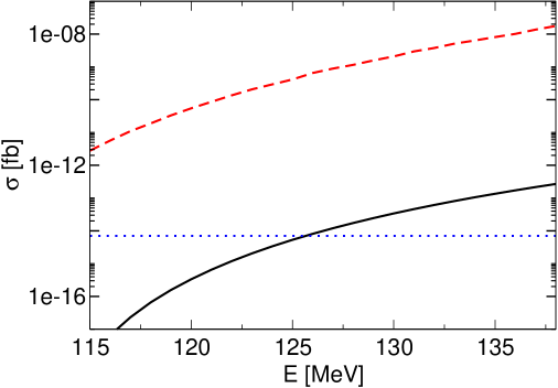
Figure 5: Total cross sections in femtobarns plotted against the energy of the incident electron beam. The solid line gives the result for production of a $\mu^{-}$ via the process $e^{-}p\rightarrow\mu^{-}p\bar{\nu}_{\mu}\nu_{e}$ (see Sec. III), and the dashed line is the result for production of a $\mu^{+}$ via the reaction $e^{-}p\rightarrow e^{-}n\mu^{+}\nu_{\mu}$ (see Sec. IV). The dotted line is the bound on BSM contributions obtained for $ep\rightarrow\mu p$ in Section II by considering the dimension-five BSM operator and the non-observation of the decay $\mu\rightarrow e\gamma$.

The dependence on energy of the total cross section for the processes $e^{-}p\rightarrow e^{-}n\mu^{+}\nu_{\mu}$ and $e^{-}p\rightarrow\mu^{-}p\bar{\nu}_{\mu}\nu_{e}$ (see Sec. III) is shown in Fig. 5. Also shown in Fig. 5 is the bound of Eq. (26) for $ep\rightarrow\mu p$ from photon exchange. Note that in Fig. 5 we do not display results for energies exceeding 140 MeV, because above that energy the $n\pi^{+}$ channel opens and $\mu^{+}$’s are copiously produced through the decay of real pions.

Even at $E_{e}=140$ MeV, the cross section for $\mu^{+}$ production via strong interactions is many orders of magnitude larger than the cross section for BSM muon conversion in Eq. (26). Indeed, it may be competitive with BSM mechanisms even if dimension-six BSM operators that induce EMU are not suppressed by, e.g. minimal lepton-flavor violation. Thus, any experiment that searches for EMU on a proton target via BSM processes should discriminate between the desired reaction and the channel $ep\rightarrow en\mu^{+}\nu_{\mu}$. Such a discrimination requires either detecting the outgoing electron, or detecting the charge of the final-state muon.

V Muon production in electron-nucleus scattering

If the proton target were replaced by a neutron target (e.g. via the use of neutrons bound inside a deuterium nucleus), the incoming electron can also interact with the neutron through its magnetic moment. From Eq. (27), the matrix element for magnetic-moment interactions introduces an extra factor—relative to the dominant charge interaction—of $q_{\mu}/M$. This translates to a factor $Q^{2}/M^{2}\approx q_{0}/M\approx 0.01$ in the cross section. Thus, the electroweak process $en\rightarrow\mu^{-}\nu_{e}\bar{\nu}_{\mu}n$ yields a smaller muon-production cross section than in the case of a proton. In contrast, the process $ep\rightarrow en\mu^{+}\nu_{\mu}$ discussed in Sec. IV is associated with an isovector matrix element at leading order in $\chi$PT, and so the cross section for production of muons will be as large for a neutron target as for a proton target. In this case the reaction is, however, $en\rightarrow ep\mu^{-}\bar{\nu}_{\mu}$. For neutrons this muon-production reaction provides a signal that cannot be distinguished from BSM electron-muon conversion by detection of the charge of the final-state muon. (As an aside, we note that in the case of $Z^{0}$ exchange, scattering off a neutron is more favorable due to its much larger weak charge as compared to the proton. However, the appearance of an extra factor of $G_{F}$ renders the cross section due to electromagnetic-weak interference terms negligible when compared to photon exchange.)

The cross section for muon production is enhanced when the electron scatters off a heavy nucleus. As an illustrative example, and to estimate the expected enhancement over the nucleonic case, we consider electron scattering on a lead nucleus (${}^{208}{\rm Pb}$). The low energy and low three-momentum transfer region is probed in conventional nuclear spectroscopy. In this region, the elastic peak appears first, although at $q_{0}^{\rm Pb}=-q^{2}/2m_{\rm Pb}$ instead of $q_{0}^{\rm prot.}=-q^{2}/2M$, so that the exchanged photon appears to be two orders of magnitude softer. In fact, though, the requirement of producing the muon implies that the photon’s virtuality is unchanged from $Q^{2}\sim m_{\mu}^{2}$; as the differential cross section scales as $\sim 1/(Q^{2})^{2}=1/(2m_{\rm Pb}q_{0}^{\rm Pb})^{2}$ considering only the effect of the heavier target yields no particular enhancement. This fact can also be verified by counting powers of the target mass and energy transfer in the expression for the differential cross section in Eq. (35).

The large charge of lead ($Z=82$) does tend to increase the cross section, although nuclear elastic form factors offset this effect substantially. The typical three-momentum transfer involved in elastic scattering is $|{\bf q}|=\sqrt{q_{0}^{2}+2m_{\rm Pb}q_{0}}\approx m_{\mu}$, which corresponds to a spatial resolution of about 2 fm. But $R_{\rm Pb}\sim 7$ fm is the typical size of the charge distribution in ${}^{208}{\rm Pb}$ as determined by fitting a conventional 2-parameter Fermi distribution for a spherical nucleus Bellicard , so we do not expect the lead nucleus to respond coherently to the electromagnetic probe. This can be quantified if we approximate the elastic form factor by the diffraction pattern from a spherical charge distribution of radius $R_{\rm Pb}$. In so doing we obtain an overall factor relative to the proton case of:

$$Z^{2}F^{2}(|{\bf q}|)\approx Z^{2}\left[\frac{3j_{1}(|{\bf q}|R_{\rm Pb})}{|{\bf q}|R_{\rm Pb}}\right]^{2}\,,$$ (51)

where $j_{1}$ is the spherical Bessel function of the first kind. For lead, $F^{2}\sim 10^{-2}$ at the $Q^{2}$’s of interest here, in good agreement with form factors extracted from data on elastic scattering from ${}^{208}{\rm Pb}$ in this region of energy and momentum transfer Frois . Therefore, if we replace the target proton by a lead nucleus, we expect an overall increase of the cross section by $Z^{2}F^{2}\sim{82}^{2}\times 10^{-2}\approx 67$.

Elastic scattering is not the complete story, however, because the maximum energy of the exchanged photon is $\sim(E_{e}-m_{\mu})\sim 30$ MeV, which is sufficient to excite a tower of collective states. Studies of inelastic form factors of the first few excited states (for example, the $3^{-}$ octupole in ²⁰⁸Pb) reveal a suppression of $\sim 10^{-2}$ or more compared to the elastic peak Kendall ; Zeigler . The width of these excited states is also small (0.1 MeV for the $3^{-}$ state), therefore, at low energies of the exchanged photon, the contribution of the elastic peak is dominant. At slightly higher energies, $q_{0}\gtrsim 10$ MeV, giant monopole and multipole resonances can be excited. These resonances are of empirical importance in studies of nuclei as they carry non-zero isospin. Although the resonances have large widths (1–5 MeV), their contribution to the cross section will also be smaller than that from the elastic peak.

Finally, we inquire whether quasi-elastic scattering should be taken into account. By quasi-elastic scattering, we are referring to those events in which a muon is produced and a nucleon is knocked out of the nucleus. This phenomenon requires the additional kinematic restriction that the three-momentum transfer exceed the Fermi momentum of the nucleon in the nucleus. Therefore, the relevant energy regime is now defined by the conditions $\Theta(|{\bf q}|-k_{F})$ and the theta functions imposed above, i.e, $\Theta(E_{e}-q_{0}-E_{\mu})$ and $\Theta((k-q-l_{2})^{2})$. These two theta functions are unchanged from the nucleonic case as they originate from the kinematics of the leptonic portion of the process, which is unaffected by changing the target from a nucleon to a nucleus. These restrictions imply that the maximum value of $(k-q-l_{2})^{2}$ is given by

$$(E_{e}-q_{0})^{2}-E_{e}^{2}-k_{F}^{2}+m_{\mu}^{2}-2m_{\mu}(E_{e}-q_{0})+2E_{e}k_{F}{\rm cos}(\hat{k}\hat{q})\geq 0\,,$$ (52)

where the inequality imposed by the theta function $\Theta((k-q-l_{2})^{2})$ is satisfied so long as $0<q_{0}<q_{0}^{<}$, where $q_{0}^{<}$ is the lesser root of the above quadratic in $q_{0}$. Clearly, this requires that $q_{0}^{<}>0$, which is equivalent to the condition

$${\rm cos}(\hat{k}\hat{q})\geq\frac{m_{\mu}}{k_{F}}+\frac{k_{F}^{2}-m_{\mu}^{2}}{2E_{e}k_{F}}\,.$$ (53)

As $|{\rm cos}(\hat{k}\hat{q})|\leq 1$, we obtain the restriction

$$E_{e}\geq\left(\frac{k_{F}+m_{\mu}}{2}\right)\,.$$ (54)

If we assume a simple picture of the nucleus with constant density $\rho\approx\rho_{\rm nuc}=0.16$ fm^-3, then $k_{F}\approx 260$ MeV, which implies that $E_{e}\geq 187$ MeV. This exceeds the pion-production threshold in ordinary electron-nucleus scattering (no muon production). It is highly desirable that the electron beam energy not be above the pion threshold at around 140 MeV, and in this case we need not include the contribution from quasi-elastic scattering, since Eq. (54) makes clear that it is important only at energies well above pion threshold. This is significantly different to the usual situation in inelastic electron-nucleus scattering (i.e. without muon production), in which pion production occurs at energies that exceed the quasielastic peak. When muon production happens, additional kinematic restrictions (viz., the energy cost of producing a muon) imply that the quasielastic peak is only important at energies that exceed the threshold for pion production. This is another distinguishing feature of the muon-production process.

VI Conclusions

We have examined the possibility of discovering physics beyond the Standard Model through lepton-flavor violation in fixed-target electron scattering. Our main findings can be summarized as:

• We have obtained a model-independent constraint on the magnitude of LFV in electron-nucleon scattering from beyond-the-Standard-Model effects using a general low-energy effective interaction with couplings constrained by experimental bounds on the nonobservance of $\mu\rightarrow e\gamma$. The cross section for LFV from the lowest-dimension operator, $\sigma<7\times 10^{-15}$ fb, is too small to be experimentally accessible with current technologies. The contribution of higher-dimension LFV operators to $ep\rightarrow\mu p$ could be larger, but is still unobservably small at present. This is in accord with similar estimates that have been made previously within specific extensions of the Standard Model Diener:2004kq ; Blazek:2004cg .

• We have identified two main sources of background in inclusive $ep$ scattering within the Standard Model when only the energy of the outgoing muon is measured, and performed detailed calculations of the relevant cross sections. The reaction $e^{-}p\rightarrow\mu^{-}\nu_{e}\bar{\nu}_{\mu}p$ is the principal background if the charge of the muon is measured, and its cross section varies from the order of $10^{-16}$ fb at incident electron energy $E_{e}=120$ MeV to $10^{-13}$ fb at $E_{e}=140$ MeV.

• If the charge of the muon is not measured, the dominant source of background comes from $\mu^{+}$s produced by the decay of virtual pions. Leading-order chiral perturbation theory gives this reaction’s total cross section $\sigma(ep\rightarrow en\mu^{+}\nu_{\mu})$ to be about $10^{-11}$ fb at incident electron energy $E_{e}=120$ MeV and $\sim 10^{-8}$ fb near the pion threshold. This background swamps any LFV signal in $ep$ scattering unless the outgoing electron is also detected or/and $\mu^{+}$ events are vetoed.

• Using a heavy nucleus as a target enhances both the desired LFV effects and the background. At the low energies carried by the exchanged photon in $e^{-}p\rightarrow\mu^{-}p\nu_{e}\bar{\nu}_{\mu}$ the role of collective nuclear excitations can be neglected in comparison to the leading effects of elastic scattering from a finite-size target. This could enhance the cross section for $e^{-}p\rightarrow\mu^{-}p\nu_{e}\bar{\nu}_{\mu}$ by as much as two orders of magnitude, but the cross section is still too small to be experimentally detectable at present.

Appendix A Phase-space evaluation for final state $p\mu\bar{\nu_{\mu}}\nu_{e}$

In this appendix, we explain how to obtain Eq. (35) from Eq. (34). We first employ a useful relation for elastic scattering

$$\int\frac{d^{3}p^{\prime}}{2E_{p^{\prime}}}\delta^{(4)}(p+q-p^{\prime})=\frac{1}{2M}\delta\left(\frac{q^{2}}{2M}+q_{0}\right)\quad{\rm where}\quad q_{0}=p_{20}^{{}^{\prime}}-p_{20}\quad\,,$$ (55)

which enables Eq. (34) to be rewritten as

$$d\sigma = \frac{2\pi}{8M^{2}E_{e}}\int\frac{d^{3}l_{2}}{(2\pi)^{3}2E_{\mu^{-}}}\int d^{4}q\int d^{4}p_{2}^{\prime}\delta^{(4)}(p_{2}-p_{2}^{\prime}-q)\delta\left(\frac{q^{2}}{2M}+q_{0}\right)$$ (56)

$$\times \int\frac{d^{3}l_{1}}{(2\pi)^{3}2E_{\nu_{\mu}}}\frac{d^{3}l_{\nu_{e}}}{(2\pi)^{3}2E_{\nu_{e}}}\delta^{(4)}(p_{2}^{\prime}-l_{1}-l_{\nu_{e}}-l_{2})\overline{|{\cal M}|^{2}}\,.$$

For massless neutrinos, the phase-space integrals over neutrino momenta in the second line of Eq. (56) can be rewritten as

$$\int d^{4}L\,\delta^{(4)}(L-p_{2}^{\prime}+l_{2})\int\frac{d^{3}l_{1}}{(2\pi)^{3}2E_{\nu_{\mu}}}\frac{d^{3}l_{\nu_{e}}}{(2\pi)^{3}2E_{\nu_{e}}}\delta^{(4)}(L-l_{1}-l_{\nu_{e}})\overline{|{\cal M}|^{2}}\,.$$ (57)

Noting from Eq. (III) that Eq. (57) has a factor $(p_{2}^{\prime}-l)\cdot l_{1}=l_{\nu_{e}}\cdot l_{1}$, the integrals over $d^{3}l_{\nu_{e}}$ and $d^{3}l_{1}$ are Jaikumar:2001hq

$$\int\frac{d^{3}l_{1}}{(2\pi)^{3}2E_{\nu_{\mu}}}\frac{d^{3}l_{\nu_{e}}}{(2\pi)^{3}2E_{\nu_{e}}}\delta^{(4)}(L-l_{1}-l_{\nu_{e}})~{}l_{\nu_{e}}.l_{1} = \frac{\pi L^{2}}{4(2\pi)^{6}}\theta(L_{0})\theta(L^{2})\,,$$ (58)

where $L^{2}=L_{0}^{2}-{\bf L}^{2}$. Using the resultant expression for Eq. (57) in Eq. (56), performing the $d^{4}L$ and $d^{4}p_{2}^{\prime}$ integrations with the aid of corresponding delta functions, and using Eq. (29), we obtain

$$d\sigma = \frac{\alpha^{2}G_{F}^{2}}{4\pi^{2}M^{2}E_{e}}\int\frac{d^{3}l_{2}}{2E_{\mu^{-}}}\int\frac{d^{4}q}{q^{4}}\delta\left(\frac{q^{2}}{2M}+q_{0}\right){\cal I}(q,l_{2})\,;$$

$${\cal I}(q,l_{2}) = (p_{2}-q-l_{2})^{2}\left[\frac{p_{2}^{\prime}.l_{2}}{{p_{2}^{\prime}}^{4}}{\cal T}_{2}-\frac{1}{2{p_{2}^{\prime}}^{2}}{\cal T}_{1}\right]_{p_{2}^{\prime}=(p_{2}-q)}\hskip-39.74872pt\Theta\left((p_{2}-q-l_{2})^{2}\right)\Theta(E-E_{\mu^{-}}-q_{0})\,.$$ (59)

where ${\cal T}_{1},{\cal T}_{2}$ are given by Eq. (III).With the aid of the only remaining delta function, the $\int d^{4}q$ can be recast as

$$\int\frac{d^{4}q}{q^{4}}\delta\left(\frac{q^{2}}{2M}+q_{0}\right){\cal I}(q,l_{2})=$$ (60)

$$M\int\frac{dq_{0}}{(-2q_{0}M)^{2}}\sqrt{q_{0}^{2}+2Mq_{0}}\,\Theta(E_{e}-E_{\mu^{-}}-q_{0})$$

$$\times \int d\Omega_{q}\Theta\left((p_{2}-q-l_{2})^{2}\right)(p_{2}-q-l_{2})^{2}\left[\frac{p_{2}^{\prime}.l_{2}}{{p_{2}^{\prime}}^{4}}{\cal T}_{2}-\frac{1}{2{p_{2}^{\prime}}^{2}}{\cal T}_{1}\right]_{(p_{2}^{\prime}=(p_{2}-q),q^{2}=-2Mq_{0})}\,.$$

The step functions $\Theta(E-q_{0}-E_{\mu^{-}})$ and $\Theta\left((p_{2}-q-l_{2})^{2}\right)$ provide the upper and lower limits on the $dq_{0}$ integral. The latter step-function also provides bounds on the angular integrations involving $d{\rm cos}\theta_{q},d\phi_{q}$. This determines the support for the various integrals as [$q_{0}^{l},q_{0}^{u}$], [${\rm cos}\theta_{q}^{l},{\rm cos}\theta_{q}^{u}$], [$\phi_{q}^{l},\phi_{q}^{u}$] and leads to (35). In our numerical calculations, we have used a constant value for $G_{F}(Q^{2}=0.01{\rm GeV}^{2})$=$1.05\times 10^{-5}$GeV^-2 as determined by its Standard-Model running in the $\overline{MS}$ scheme Czarnecki:2000ic .

Appendix B Numerical notes

The integrals in Eq. (35) are performed as follows. We choose the $+\hat{z}$ axis to be along the electron beam direction. The polar angle $\theta_{\mu}$ is measured from the $+\hat{z}$-axis in the vertical plane containing this axis. The azimuthal angle $\phi_{\mu}$ is measured anti-clockwise from the (arbitrary) $-\hat{z}$ axis in a plane containing this axis. The position of the detected muon is then uniquely specified by the angles $\theta_{\mu}$ and $\phi_{\mu}$. Once the position of the muon is specified as above, for a fixed momentum $p_{\mu}$ we can determine the range of $q_{0}$ for which the step functions in Eq. (35) do not vanish. This procedure determines the bounds on $\cos\theta_{q}$ at fixed beam energy $E_{e}$, from which bounds on $\phi_{q}$ follow. The numerical evaluation of the multiple integral is then performed using standard quadrature methods. At the low $Q^{2}$ values involved here the $Q^{2}$-dependence of $G_{E}$ and $G_{M}$ induces a correction of 5–10% in the cross section, as compared to using their $q^{2}=0$ values. We have taken this into account in the numerical results presented in Sec. III, using a standard dipole parameterization obtained from studies of $e^{-}p$ scattering:

$$G_{E}(Q^{2})=\frac{G_{M}(Q^{2})}{1+\kappa}=\frac{1}{\left(1+Q^{2}/0.71{\rm GeV}^{2}\right)^{2}}\,\quad.$$ (61)

For the range of $Q^{2}$ relevant to the process considered here, this parameterized form is accurate to better than 1%.

References

• (1) G. L. Fogli, E. Lisi, A. Marrone, and A. Palazzo, Prog. Part. & Nuc. Phys. 57, 742 (2006).
• (2) K. P. Diener, Nucl. Phys.  B 697, 387 (2004) [arXiv:hep-ph/0403251].
• (3) T. Blazek and S. F. King, arXiv:hep-ph/0408157.
• (4) S. Ritt [MEG Collaboration], Nucl. Phys. Proc. Suppl.  162, 279 (2006).
• (5) I. Sick, Phys. Lett.  B 576, 62 (2003).
• (6) T. P. Cheng and L. F. Li, “Gauge Theory Of Elementary Particle Physics,” (Clarendon, Oxford, UK, 1984)
• (7) W. M. Yao et al. [Particle Data Group], J. Phys. G 33, 1 (2006).
• (8) V. Cirigliano, B. Grinstein, G. Isidori and M. B. Wise, Nucl. Phys.  B 728, 121 (2005).
• (9) R. G. Sachs, Phys. Rev. Lett. 12, 231 (1964).
• (10) F. Halzen and A. D. Martin, ”Quarks and Leptons: Introductory Course in Modern Particle Physics”, © 1984, John Wiley & Sons.
• (11) V. Bernard and U.-G. Meißner, Ann. Rev. Nucl. Part. Sci. 57, 33 (2007).
• (12) H. W. Fearing, T. R. Hemmert, R. Lewis and C. Unkmeir, Phys. Rev.  C 62, 054006 (2000).
• (13) J. F. Donoghue, E. Golowich and B. R. Holstein, “Dynamics Of The Standard Model,” (Cambridge University Press, New York, 1994).
• (14) J. Gasser, M. E. Sainio and A. Svarc, Nucl. Phys.  B 307, 779 (1988).
• (15) R. Mertig, M. Bohm and A. Denner, Comput. Phys. Commun.  64, 345 (1991).
• (16) J. B. Bellicard and K. J. van Oostrum, Phys. Rev. Lett. 19, 242 (1967).
• (17) B. Frois et al, Phys. Rev. Lett. 38, 152, (1977).
• (18) H. Crannell, R. Helm, H. Kendall, J. Oeser and M. Yearian, Phys. Rev. 123, 923 (1961).
• (19) J. F. Zeigler and G. A. Peterson, Phys. Rev. 165, 1337 (1968).
• (20) P. Jaikumar and M. Prakash, Phys. Lett.  B 516, 345 (2001) [arXiv:astro-ph/0105225].
• (21) A. Czarnecki and W. J. Marciano, Int. J. Mod. Phys.  A 15, 2365 (2000) [arXiv:hep-ph/0003049].