Dynamic Boundaries of Event Horizon Magnetospheres

Abstract

This Letter analyzes 3-dimensional simulations of Kerr black hole magnetospheres that obey the general relativistic equations of perfect magnetohydrodynamics (MHD). Particular emphasis is on the event horizon magnetosphere (EHM) which is defined as the the large scale poloidal magnetic flux that threads the event horizon of a black hole (This is distinct from the poloidal magnetic flux that threads the equatorial plane of the ergosphere, which forms the ergospheric disk magnetosphere). Standard MHD theoretical treatments of Poynting jets in the EHM are predicated on the assumption that the plasma comprising the boundaries of the EHM plays no role in producing the Poynting flux. The energy flux is electrodynamic in origin and it is essentially conserved from the horizon to infinity, this is known as the Blandford-Znajek (B-Z) mechanism. To the contrary, within the 3-D simulations, the lateral boundaries are strong pistons for MHD waves and actually inject prodigious quantities of Poynting flux into the EHM. At high black hole spin rates, strong sources of Poynting flux adjacent to the EHM from the ergospheric disk will actually diffuse to higher latitudes and swamp any putative B-Z effects. This is in contrast to lower spin rates, which are characterized by much lower output powers and modest amounts of Poynting flux are injected into the EHM from the accretion disk corona.

The long term 3-D simulations discussed in De Villiers et al (2003, 2005); Hirose et al (2004); Krolik et al (2005); Hawley and Krolik (2006) (HK, hereafter) offer an important virtual laboratory for studying the physics of black hole driven jets. These simulations readily evolve to a configuration with a net accreted poloidal magnetic flux that is trapped within the accretion vortex or funnel. This region is the black hole magnetosphere and it supports a jet dominated by electromagnetic energy for rapidly rotating black holes. In a previous paper, Punsly (2007), it was shown that the physics conducive to an ergospheric disk (first described in Punsly and Coroniti (1990)) existed in the high spin simulation, $a/M=0.99$ (where the black hole mass, $M$, and the angular momentum per unit mass, $a$, are in geometrized units), known as KDJ. The ergospheric disk jet (EDJ) is launched from the plasma near the equatorial plane of the ergosphere. The event horizon magnetosphere (EHM) is comprised of poloidal flux that threads the event horizon (see the middle frame of figure 1). This paper explores the sources of Poynting flux in the EHM in the context of the 3-D simulations. In the EHM, there are four possible sources of Poynting flux that follow from energy conservation.

1. Energy can be transferred from the plasma to the electromagnetic field. However, the EHM is virtually evacuated of plasma due to the centrifugal barrier and there is little energy to transfer to the field in perfect MHD.

2. Any other sources must be surface terms at the boundary of the EHM. The first possibility is the electrodynamic component that is associated with the event horizon boundary surface. This is customarily called the Blandford-Znajek (B-Z) effect Blandford and Znajek (1977).

3. The second boundary surface, which is associated with the EDJ, is the equatorial accretion flow in the ergosphere.

4. Outside the ergosphere, the EHM is bounded by the accretion disk and the disk corona. A source on this boundary will be called a coronal piston (see figure 2).

It has been typically assumed that a Poynting jet in the EHM is confirmation of a B-Z process at work. However, it will be shown that the two simulations, KDJ with $a/M=0.99$ and KDH with $a/M=0.95$, indicate that this can be a misleading interpretation in general. The energy output of KDJ is dominated by the EDJ Punsly (2007). KDH provides an interesting contrast to KDJ, because the EDJ is not nearly as powerful as it is in KDJ in the late time data slices. In KDJ, the Poynting flux in the EHM at large distances from the hole, $r\sim 100M$, is dominated by the energy flux from the EDJ that is gradually diffusing to higher latitudes within the funnel as it propagates outward. For KDH, the coronal piston that was discussed in HK in the context of driving the enormous mass flux in the ”funnel wall jet” also injects significant amounts of Poynting flux into the funnel as a second order effect.

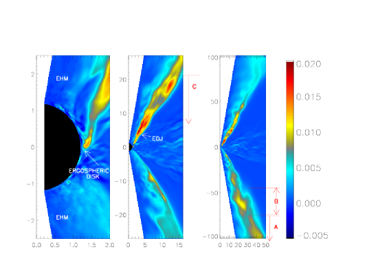
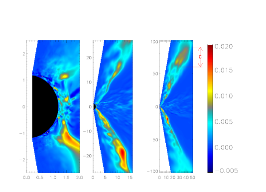
Figure 1: The Poynting flux in KDJ. The color bar is in code units. The rows are in chronological order, t= 9840 M (top), t=9920 M (middle) and t= 10000 M (bottom). There is no data clipping, saturated regions are white. The region $r<r_{in}=1.203M$ is black and $r_{+}=1.141M$.

1 The 3-D Simulations

J. Krolik and J. Hawley have generously shared the data for the last three time slices of KDH and KDJ, at t = 9840 M, t= 9920 M and t=10000 M. The simulations are performed in the Kerr metric (that of a rotating, uncharged black hole), $g_{\mu\nu}$. Calculations are carried out in Boyer-Lindquist coordinates $(r,\theta,\phi,t)$. The reader should refer to HK and references therein for details of the simulations. We only give a brief overview of the most relevant details. The initial state is a torus of gas in equilibrium that is threaded by concentric loops of weak magnetic flux that foliate the surfaces of constant pressure. The magnetic loops are twisted azimuthally by the differentially rotating gas. This creates significant magnetic stress that transfers angular momentum outward in the gas, initiating a strong inflow that is permeated by magneto-rotational instabilities (MRI). The end result is that after t = a few hundred M, accreted poloidal magnetic flux gets trapped in the accretion vortex or funnel (with an opening angle of $\sim 60^{\circ}$ at the horizon tapering to $\sim 30^{\circ}-35^{\circ}$ at $r>20M$). This region is the black hole magnetosphere and it supports Poynting flux. The surrounding accretion flow is very turbulent. The strong transients die off by t = 2000 M, so the late time data dumps are the most physically relevant Hawley and Krolik (2006).

Numerically, the problem is formulated on a grid that is 192 x 192 x 64, spanning $r_{in}<r<120M$, $8.1^{\circ}<\theta<171.9^{\circ}$ and $0<\phi<90^{\circ}$. The inner calculational boundary, $r_{in}$, is located close to, but just outside of the event horizon, $r_{+}$, where the coordinates are singular. The $\phi$ boundary condition is periodic and the $\theta$ boundary conditions are reflective. Zero-gradient boundary conditions are employed on the radial boundaries, where the contents of the active zones are copied into the neighboring ghost zones. MHD waves propagate slower than the speed of light, therefore the gravitational redshift creates a magneto-sonic critical surface outside of $r_{+}$ from which no MHD wave can traverse in the outward direction Punsly (2001). The philosophy was to choose $r_{in}$ to lie inside the magneto-sonic critical surface, thereby isolating it from the calculational grid. There are also steep gradients in the metric derived quantities as $r_{+}$ is approached. This is handled by increasing the resolution of the grid near $r_{in}$ with a cosh distribution of radial nodes. The validity of the numerics of this method was verified, near $r_{in}$, in De Villiers and Hawley (2003) by comparing simulations to simple analytic solutions. Even so, the simulations are closely monitored to look for unnatural boundary reflections. We also note the 3-D simulations in Kerr-Schild coordinates (which are nonsingular on the horizon) in Fragile et al (2007). To test the code, they ran simulations of magnetized tori that were initiated from identical input parameters to those used by Hawley et al. In the words of C. Fragile (private communication), the results were ”remarkably similar.” Even though this was only verified for a/M=0.9, it is compelling. Consequently, for the purposes of this study it was concluded that the numerics were reliable inside the ergosphere.

2 The KDJ Simulation

The conservation of global, redshifted, energy flux, defined in terms of the stress-energy tensor, is simply, $\partial(\sqrt{-g}\,T_{t}^{\,\nu})/\partial(x^{\nu})=0$ (Punsly, 2007). The four-momentum $-T_{t}^{\,\nu}$ has two components: one from the fluid, $-(T_{t}^{\,\nu})_{\mathrm{fluid}}$, and one from the electromagnetic field, $-(T_{t}^{\,\nu})_{\mathrm{EM}}$. The quantity $g=-(r^{2}+a^{2}\cos^{2}{\theta})^{2}\sin^{2}{\theta}$ is the determinant of the metric. The integral form of the conservation law arises from the trivial integration of the partial differential expression Thorne et al (1986). It follows that the poloidal components of the redshifted Poynting flux are $S^{\theta}=-\sqrt{-g}\,(T_{t}^{\,\theta})_{\mathrm{EM}}$ and $S^{r}=-\sqrt{-g}\,(T_{t}^{\,r})_{\mathrm{EM}}$. We can use these simple expressions to understand the EHM Poynting jet in KDJ. Figure 1 is a plot of $S^{r}$ in KDJ viewed at three different levels of magnification, at t= 9840 M (top row), t= 9920 M (middle row) and the bottom frames are at t = 10000 M. Each frame is the average over azimuth of each time step. This greatly reduces the fluctuations as the accretion vortex is a cauldron of strong MHD waves. The individual $\phi=\mathrm{constant}$ slices show the same dominant behavior, however it is embedded in large MHD fluctuations. The left hand column shows strong beams of $S^{r}$ coming from near the black hole. In Punsly (2007), it was shown that the source of these beams was $S^{\theta}$ that was created by the ergospheric disk. The base of the EDJ emerging from the dense equatorial plasma is well resolved in both $r$ and $\theta$ with $\approx 20$ and $>30$ grid zones, respectively.

In this paper, we turn our attention to the propagation of individual flares from the ergospheric disk out to the outer calculational boundary at $r=120M$. Even though the time sampling is very coarse in the data dumps ($\Delta t=80M$), we can understand the propagation of the EDJ because of the wide angle views available in the right hand column of figure 1. We track the EDJ evolution by identifying the strong knots or flares in figure 1 based on the following reasoning. As discussed in Punsly (2001), the $S^{r}$ flares will propagate at the speed of an MHD discontinuity as modified by the plasma bulk flow velocity. The plasma near the edge of the vortex has accelerated to $v_{r}>0.9c$ by r= 30 M. So the flares of $S^{r}$ should propagate radially at $V_{flare}\,\mbox{\raisebox{-2.58334pt}{$\stackrel{{\scriptstyle\textstyle<}}{{\sim}}$}}\,c$ for $r>30M$. Without having the benefit of the detailed time evolution, this upper bound is the best estimate that we can make for $V_{flare}$. First, consider the strong knot, ”C,” at t=10000 M in the right hand frame. Label the outer radial extent of knot C at t = 10000 M by $r_{+C}(t=10000M)=100.9M$ and inner radial edge by $r_{-C}(t=10000M)=65.9M$. Translating this MHD discontinuity back in time to t = 9920 M is equivalent to a radial displacement $V_{flare}\Delta t=V_{flare}(-80M/c)\,\mbox{\raisebox{-2.58334pt}{$\stackrel{{\scriptstyle\textstyle>}}{{\sim}}$}}\,-80M$. Thus at t= 9920M, knot ”C” should extend from the ergospheric disk to $r_{+C}(t=9920M)\,\mbox{\raisebox{-2.58334pt}{$\stackrel{{\scriptstyle\textstyle>}}{{\sim}}$}}\,20.9M$. This is verified by the red patches in the middle frame at t=9920 M.

Next consider the strong knot, ”A,” at t= 9840 M in the right hand frame. Label the outer radial extent of knot A at t = 9840 M by, $r_{+A}(t=9840M)=58.9M$ and inner radial edge by $r_{-A}(t=9840M)=22.0M$. Time translating this feature to t = 9920 M implies that $r_{-A}(t=9920M)\,\mbox{\raisebox{-2.58334pt}{$\stackrel{{\scriptstyle\textstyle<}}{{\sim}}$}}\,102.0M$, so it must be visible near the edge of the right hand frame at t = 9920 M. Furthermore, unless the flare is propagating inordinately slowly, $V_{flare}<0.75c$, $r_{+A}(t=9920M)$ will be beyond the outer boundary of the plot. There is only one plausible feature at t =9920 M. Finally, there is a strong flare ”B” that is emerging from the ergospheric disk at t = 9840 M in the left and middle frames. Thus, at t = 9920 M, some portion of the flare must be within 80 M of the black hole, hence the identification of ”B” in the right hand frame.

Figure 1 demonstrates a type (iii) source in the notation of the introduction. At $r\approx 1.5M-2.0M$, the EDJ enters the EHM from the periphery (left hand frames). The EDJ gets quickly linked into the EHM because the ergopsheric disk magnetosphere in KDJ is comprised of small patches of twisted vertical flux that become intertwined with the large-scale flux in the EHM on scales of $\sim$ 1M - 2M (Punsly, 2007). After this rapid injection, the $S^{r}$ in the EDJ keeps spreading towards the pole as it propagates outward. At the time steps that were made available to this author, the EDJ is the predominant source of $S^{r}$ in the EHM. By $r\approx 100M$, the EDJ is flooding the EHM, even close to the polar axis (it should be noted that the total energy flux is larger than $S^{r}$, $\approx 20\%$ is in mechanical form in the EHM at $r\approx 100M$). The relevance to this discussion is that the EHM is inundated with $S^{r}$ that was not created on field lines that thread the horizon, but on flux entrapped within the equatorial accreting plasma. The slow diffusion of $S^{r}$ poleward at $r>30M$ is most likely regulated by numerical diffusion. This might seem like a problem from a numerical point of view, but physically this is not nearly as much of a concern from a qualitative standpoint. Perfect MHD is just a simple tractable method of dealing with the plasma physics. A realistic, high temperature, jet plasma is likely to have anomalous resistivity from a variety of sources, Somov and Oreshina (2000); Treumann (2001), and the diffusion of field energy should naturally occur. The simulation cannot accurately describe the diffusion rate. However, qualitatively speaking it indicates that if the jet propagates extremely far from the hole ($r\gg 120M$), regardless of the exact details of the diffusion microphysics, the EDJ energy flux is likely to get smeared out towards the polar region.

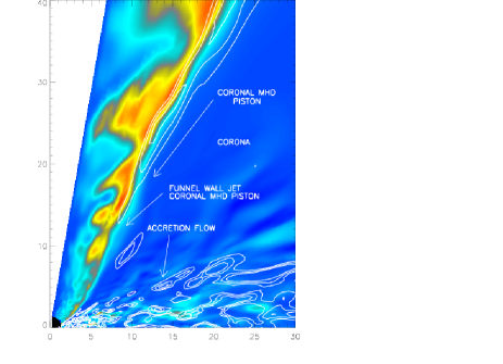
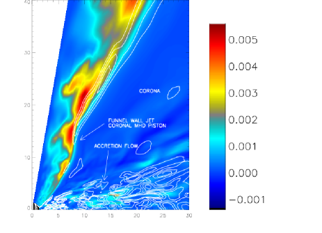
Figure 2: The coronal MHD piston is illustrated by these plots of the Poynting flux in KDH. The color bar is in code units. The frames are in chronological order, t= 9840 M (left), t=9920 M (center) and t= 10000 M (right). There is no data clipping, saturated regions are white. The overlayed white contours represent, $P_{r}$, the radial momentum flux described in the text. At each coronal piston location there is a large pressure flare, see figure 3. Inside of $r_{in}=1.403M$ ($r_{+}=1.312M$) is black.

3 The KDH Simulation

There is a relatively weak EDJ in KDH that is noticeable at t = 9840 M, but it is otherwise negligible. This circumstance allows for the detection of weaker sources of $S^{r}$ that would otherwise be swamped by a strong EDJ. Figure 2 is a plot of $S^{r}$ for these three time slices in chronological order, going from left to right. Each frame is the average over azimuth of the time step. The contours of the radial momentum flux due to mass motion, $P_{r}\equiv\sqrt{-g}\rho U^{r}U_{r}$ (where $\rho$ is the proper density and $U^{\mu}$ is the four velocity), is overlayed in white in order to define the location of the ”funnel wall jet,” as was done in HK. The funnel wall jet is a shear layer between the accretion disk corona and the Poynting jet. It is a collimated sub-relativistic flow that transports most of the mass outflow in the jetted system. In HK, it was shown to be driven by the total pressure (gas plus magnetic) gradient in the corona that is oblique to the funnel wall boundary. The gas in this region is constrained from being pushed into the funnel by the centrifugal barrier. The component of pressure gradient that is parallel to the centrifugal barrier forces the flow to be squeezed outward as a shear layer.

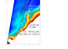
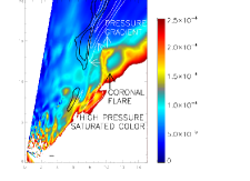
Figure 3: A closeup of the coronal piston at t =10000 M is depicted in these plots of the total pressure density (gas plus magnetic), expressed in terms of the gas pressure $P_{g}$ and the Faraday tensor as $\sqrt{-g}(P_{g}+F^{\mu\nu}F_{\mu\nu}/16\pi)$. The left frame is averaged over $\phi$ and the right frame is at $\phi=49.2^{\circ}$. The color bar is the strength of the total pressure in code units. High pressure regions of the corona are saturated and appear white. The force associated with the pressure gradient is indicated by the white arrows. The overlayed white contours represent, $P_{r}$, the radial momentum flux as in figure 2 and the black contours represent $S^{r}$.

In figure 2, there is an almost one to one correspondence, between locations where $P_{r}$ of the funnel wall jet increases and sites where $S^{r}$ increases at the funnel wall boundary in the EHM. It is the coronal pressure and not the outgoing Poynting jet (OPJ, hereafter) that drives the funnel wall jet. Figure 3 shows a strong flare in the total pressure (gas plus magnetic) at t =10000 M. The pressure gradient seems to provide the accelerating force that drives $P_{r}$. The flare appears to be a high pressure loop emerging from the corona, as evidenced by the right hand frame of figure 3. The loop location and topology are inconsistent with the high pressure feature being injected into the corona from the funnel interior. The magnetic pressure in the corona actually exceeds the magnetic pressure in the EHM at these intermediate radii, $10M<r<30M$, precisely the region where the flares tend to occur. Table 4 of HK indicates that $\overline{S_{in}}\equiv\int_{r=r_{in}}S^{r}\,d\theta d\phi dt\equiv\int S^{r}_{in}\,d\theta=(2.79/4.26)P_{jet}$, where $P_{jet}$ is the total energy transported to $r=120M$ by the funnel wall jet. Table 4 also indicates that $\int_{r=120M}S^{r}\,d\theta d\phi dt$ = (1.46/2.79) $\overline{S_{in}}$. Therefore, by conservation of energy, a putative B-Z effect can provide at most $(2.79-1.46)/4.26=0.31$ of $P_{jet}$, and is too feeble to drive the funnel wall jet.

Most of $\overline{S_{in}}$ is directed into the equatorial accretion flow and never reaches the plasma in the OPJ. To see this, we summarize figure 5 of HK. There are broad relative maxima in $S^{r}_{in}$ at $\theta<41.3^{\circ}$ ($\theta>137^{\circ}$), but $S^{r}_{in}$ decreases rapidly with $\theta$ and $S^{r}_{in}<0$ when $41.3^{\circ}<\theta<54.5^{\circ}$ ($120.4^{\circ}<\theta<137^{\circ}$). The two strongest maxima in $S^{r}_{in}$ are in the equatorial accretion flow at $\theta\approx 80^{\circ}$ ($\theta\approx 100^{\circ}$) and this energy never reaches the OPJ. Therefore, it is unclear how the region $41.3^{\circ}<\theta<137^{\circ}$ is related to the B-Z mechanism. In order to understand the global energy budget, we want to know how much $\overline{S_{in}}$ reaches the OPJ. Based on the available data, we can generate an upper bound. First, we define the OPJ as in Hirose et al (2004) by the magnetic dominance condition, defined in terms of the Faraday field strength tensor as $F^{\mu\nu}F_{\mu\nu}/(16\pi\rho h)>1$ ($h$ is the enthalpy per unit mass) and $U^{r}>0$. Virtually all the $S^{r}$ that reaches $r=120M$ in the available KDH time slices flows in the OPJ as defined above. Inspecting our three time slices, the OPJ initiates at $r_{min}<3M$, with an angular extreme near the base given by $\theta_{max}\approx 55^{\circ}$ ($\theta_{min}\approx 125^{\circ}$), in agreement with the time averaged data in figure 11 of Hawley and Krolik (2006). The OPJ is collimated, i.e., $d\theta_{max}/dr<0$ for $\theta<90^{\circ}$ ($d\theta_{min}/dr>0$ for $\theta>90^{\circ}$). In each of the time slices, we can compare $\int S^{r}d\theta d\phi$ near $r_{in}$ above the equatorial accretion flow to $\int S^{r}d\theta d\phi$ in the OPJ to assess how much $\overline{S_{in}}$ reaches the OPJ. The simulations have significant fluctuations. Averaging over r smooths out the spatial fluctuations and is a more reliable diagnostic than computing fluxes at a single radius. Unfortunately, there is not enough data to perform a meaningful time average. In each time slice we find $\frac{1}{0.597M}\int^{2M}_{r_{in}}\,dr\int^{\theta=70^{\circ}}_{\theta=8.1^{\circ}}S^{r}\,d\theta d\phi>\frac{1}{4M}\int^{9M}_{5M}\,dr\int^{\theta=\theta_{max}}_{\theta=8.1^{\circ}}S^{r}\,d\theta d\phi$; $\frac{1}{0.597M}\int^{2M}_{r_{in}}\,dr\int^{\theta=171.9^{\circ}}_{\theta=110^{\circ}}S^{r}\,d\theta d\phi>\frac{1}{4M}\int^{9M}_{5M}\,dr\int^{\theta=171.9^{\circ}}_{\theta=\theta_{min}}S^{r}\,d\theta d\phi$. The 6 inequalities tend to indicate that $\overline{S_{in}}$ at $\theta<70^{\circ}$ ($\theta>110^{\circ}$) is larger (the average excess is $20\%$) than the total $S^{r}$ flowing through the OPJ at $r\approx 7M$, $\theta<50^{\circ}$ ($\theta>130^{\circ}$) and some of the $\overline{S_{in}}$ at $\theta<70^{\circ}$ is absorbed by the accretion disk and corona at $r\leq 7M$, $\theta>50^{\circ}$ ($\theta<130^{\circ}$). This excess is apparently large enough to persist in spite of significant temporal variations. Conversely, the probability of the hypothesis that random temporal fluctuations have conspired to mask what is actually a conserved energy flow from $r_{in}$, $\theta<70^{\circ}$ ($\theta>110^{\circ}$) to the OPJ at $r\approx 7M$ is rejected at the (0.5 per hemisphere) $1-(0.5)^{6}=0.9844$ significance level. Integrating the area under the plot of $S^{r}_{in}$ in figure 5 of HK, one finds that only 39% of the total $\overline{S_{in}}$ originates in the angular range $8.1^{\circ}<\theta<70^{\circ}$, $110^{\circ}<\theta<171.9^{\circ}$. Thus, the data tends to show that $0.39\overline{S_{in}}$ is a loose upper limit to the maximum amount of $\overline{S_{in}}$ that can reach the OPJ. Applying this to the results in table 4 of HK implies that $>[1.46-(0.39)(2.79)]/1.46=0.26$ of the $S^{r}$ in the OPJ at $r=120M$ is created at $r>r_{in}$ during the course of the simulation. Furthermore, integrating over the funnel cross section at both $r_{in}$ and across the flares, $[\int^{\theta=35^{\circ}}_{\theta=8.1^{\circ}}S^{r}\,d\theta d\phi]_{\mathrm{flare}}>1.5(1/0.597M)\int^{2M}_{r_{in}}\,dr\int^{\theta=70^{\circ}}_{\theta=8.1^{\circ}}S^{r}\,d\theta d\phi$ in the last two time steps (there is a weak EDJ at t =9820 M that skews our results, so it is omitted from this analysis). If one includes the mechanical energy flux as well, there is consistently more than twice the total energy flux in the strong flares then there is total energy flux through $r_{in}$, $\theta<70^{\circ}$. This suggests that coronal injection sites are sufficiently strong to make up this apparent $>26\%$ deficit in $S^{r}$.

One might be concerned that there are only $\approx 8$ -10 angular zones between the coronal piston and the funnel and this leads to significant numerical diffusion. From a numerics point of view this is much more of a concern than from a physical point of view. The MHD code is just a simple approximation to any real turbulent plasma state. The turbulent corona is likely to have an anomalous resistivity and diffusion should occur Somov and Oreshina (2000); Treumann (2001). The rate of diffusion cannot be determined by this simulation. However, the qualitative idea that a strong flare in coronal energy can in principle reach the funnel interior is strongly indicated.

4 Discussion

The philosophy of this paper is not that the simulations of idealized magnetized tori gives us a direct picture that can be applied to AGN central engines. They are treated only as virtual laboratories to see what effects might self-consistently occur near a magnetized black hole. These simulations have led us to a new realization, the boundaries of the EHM should be dynamic and are not likely to be passive boundary surfaces for the magnetic field. It was shown that electrodynamic energy flux can arise in the EHM as a result of sources radiating energy from the lateral boundaries. Even if the EHM can be construed as ”force-free,” the dynamics of the lateral boundaries are determined by strong inertial forces that should make them strong MHD pistons. This circumstance was not anticipated in theoretical treatments of electrodynamic jets in the EHM Blandford and Znajek (1977); Phinney (1983). The fact that electromagnetic energy can come into the EHM from the side goes right to the heart of the assumptions in the B-Z solution. The B-Z solution is the perfect MHD solution in which energy conservation reduces to Poynting flux conservation from the horizon to a relativistic wind at asymptotic infinity Phinney (1983). From this condition, the parameters of the field are uniquely determined for a given poloidal field distribution, in particular the field line angular velocity, $\Omega_{F}$, and the total electromagnetic energy output from the black hole, $\int S^{r}\,d\theta d\phi$. If there are strong sources of Poynting flux along the lateral walls of the EHM, the spacetime near the event horizon can not adjust the system to enforce the B-Z field parameters within the EHM. This is a direct consequence of the fact that the plasma near the event horizon in the EHM can not effectively react back on the outgoing wind or jet and modify its electromagnetic properties because of the gravitational redshifting of the MHD characteristics Punsly (2001); Punsly and Bini (2004). The plasma near the horizon in the EHM will passively accept any field parameters imposed by the EDJ and the accretion disk corona (Punsly, 2001). As such, in a general astrophysical context, the basic parameters such as $\Omega_{F}$ and $\int S^{r}\,d\theta d\phi$ are indeterminant. Of course, this does not preclude the possibility of an MHD numerical system evolving towards B-Z, if the numerical problem is properly constructed Komissarov (2004). From a physical point of view, the strong forces that are responsible for compressing the flux down to the horizon still reside in the ”funnel walls,” rendering the lateral boundaries as strong MHD pistons. In a realistic astrophysical setting, inertial forces in the lateral boundaries are likely to play an important role, or even a dominant role, in the determination of the jet power from the EHM.

References

- Blandford and Znajek (1977) Blandford, R. and Znajek, R. 1977, MNRAS. 179, 433
- De Villiers and Hawley (2003) De Villiers, J., Hawley, 2003, ApJ 589, 458
- De Villiers et al (2003) De Villiers, J., Hawley, J., Krolik, 2003, ApJ 599,1238
- De Villiers et al (2005) De Villiers, J., Hawley, J., Krolik, K.,Hirose, S. 2005, ApJ 620, 878
- Fragile et al (2007) Fragile, C., Blaes,O., Anninos, P., Salmonson, J. 2007, to appear in ApJ, http://xxx.lanl.gov/abs/0706.4303
- Hawley and Krolik (2006) Hawley, J., Krolik, J. 2006, ApJ 641, 103 HK
- Hirose et al (2004) Hirose, S., Krolik, K., De Villiers, J., Hawley, J. 2004, ApJ 606, 1083
- Komissarov (2004) Komissarov, S. 2004, MNRAS350, 1431
- Krolik et al (2005) Krolik, K., Hawley, J., Hirose, S. 2005, ApJ 622, 1008
- Phinney (1983) Phinney, E.S. 1983, PhD Dissertation University of Cambridge.
- Punsly (2001) Punsly, B. 2001, Black Hole Gravitohydromagnetics (Springer-Verlag, New York)
- Punsly (2007) Punsly, B. 2007, ApJL 661, 21
- Punsly and Bini (2004) Punsly, B. and Bini, D. 2004, ApJL 601, 135
- Punsly and Coroniti (1990) Punsly, B. and Coroniti, F. 1990, ApJ 354, 583
- Somov and Oreshina (2000) Somov, B., Oreshina, A. 2000, A& A354 703.
- Thorne et al (1986) Thorne, K., Price, R. and Macdonald, D. 1986, Black Holes: The Membrane Paradigm (Yale University Press, New Haven)
- Treumann (2001) Treumann, R. 2001, Earth, Planets & Space 53 453.