Probing Little Higgs Model in $e^{+}e^{-}\rightarrow\nu\bar{\nu}\gamma$ Process

Abstract

We study the process $e^{+}e^{-}\rightarrow\nu\bar{\nu}\gamma$ to search for its sensitivity to the extra gauge bosons $Z_{2}$, $Z_{3}$ and $W_{2}^{\pm}$ which are suggested by the little Higgs models. We find that the ILC with $\sqrt{s}=0.5$ TeV and CLIC with $\sqrt{s}=3$ TeV cover different regions of the LHM parameters. We show that this channel can provide accurate determination of the parameters, complementary to measurements of the extra gauge bosons at the coming LHC experiments.

I Introduction

Despite the impressive success of the Standard Model (SM) in describing all existing experimental data at currently available energies, it contains many unsolved problems. For example, origin of the fermion mass, origin of the CP violation, hierarchy problems, etc. Therefore, it is commonly believed that SM is low energy manifestaion of more fundamental theory. In order to solve the hierarchy and fine-tuning problems between the electroweak scale and the Planck scale, new physics at the TeV scale is expected. In coming years the Large Hadron Collider (LHC) and later International Linear Collider (ILC) will provide us detailed information about the electroweak symmetry breaking and the origin of the hierarchy of fermion masses and CP-violating interactions. The supersymmetry introduces an extended space-time symmetry and removes the quadratically divergent corrections due to the superpartners of fermions and bosons. Extra dimensions reinterpret the problem completely by lowering the fundamental Planck scale. Technicolor theories introduce new strong dynamics at scale not much above the electroweak scale, thus defer the hierarchy problem. Among the most popular non-supersymmetric model for solving hierarchy problem in so-called little Higgs model Arkani02 (1) (see for example Han03 (2) and references therein). It is expected that the global symmetry breaking scale $\lesssim 10$ TeV in order for the little Higgs model to be relevant for the hierarchy. The little Higgs model solves the problem at one-loop level by eliminating the quadratic divergencies via the presence of a partially broken global symmetry $SU(5)$. The masses of these gauge bosons are expected to be order of global symmetry breaking scale $f$ for $SU(5)\to SO(5)$. In other words, the new heavy particles in this model cancel the quadratic divergencies in question. The subgroup $[SU(2)\times U(1)]^{2}$ is also broken into $SU(2)_{L}\times U(1)_{Y}$ group of the SM at the scale $f$ of a few TeV and then $U(1)_{em}$ at the Fermi scale $v\simeq 246$ GeV. The minimal type is the ’Littlest Higgs Model’ (LHM), in addition to the SM particles new charged heavy vector bosons $W_{2}^{\pm}$ (or heavy $W_{H}^{\pm}$), two neutral vector bosons $Z_{2}$ (or heavy $Z_{H}$) and $Z_{3}$ (or heavy photon $A_{H}$), a heavy top quark ($T$) and a triplet of scalar heavy particles ($\phi^{\pm},\phi^{0}$) are present.

Since the LHM predicts many new particles, then search of these particles usually are performed in two different way: i) via their indirect effects, i.e. these particles new at loop and change SM predictions on flavor changing neutral current processes (FCNC), ii) their direct productions in high energy colliders. The relevant scale $f$ of new physics must be $\gtrsim 2-3$ TeV in order to be consistent with the electroweak precision data Csaki03 (3, 4, 5, 6). Consequence of littlest Higgs model in rare FCNC $B$ and $K$ decays comprehensively studied in the works Blanke07 (4). Direct productions of new particles in high energy colliders are discussed in the works Kai07 (5). The direct production of new heavy gauge bosons are kinematically limited by the available center of mass energy of the present colliders. At the Large Hadron Collider (LHC), the possible signals of extra gauge bosons would show up through peaks in the invariant mass distributions of their decay products Azuelos04 (7).

In present work, we study the indirect effects of extra gauge bosons in the cross sections of the process $e^{+}e^{-}\rightarrow\nu\bar{\nu}\gamma$ at high energy linear $e^{+}e^{-}$ colliders; namely, International Linear Collider (ILC) ILC (8) and Compact Linear Collider (CLIC) CLIC (9). In additon to the limits from hadron colliders, an improvement on the sensitivity of the physical observables will be reached at future $e^{+}e^{-}$linear colliders. Finally, we discuss how accurately the LHM parameters will be measurable at the ILC and CLIC.

II Theoretical framework

The process $e^{+}e^{-}\to\nu\bar{\nu\gamma}$ is widely discussed in connection of determination of number of neutrino Ma78 (10) and understanding dynamics of stellar processes. Before discussion of the $e^{+}e^{-}\to\nu\bar{\nu}\gamma$ process in the LHM few illuminating remarks about main ingredients of the LHM are in order. In the little Higgs model in addition to the standard $W^{\pm}$ and $Z$ boson contributions there are contributions coming from new heavy vector bosons, i.e. from extended gauge sector. The kinetic term of the scalar field $\Sigma$ in lagrangian has the form Arkani02 (1)

$$L=\frac{f^{2}}{8}Tr\left|D_{\mu}\Sigma\right|^{2}$$ (1)

with the covariant derivative of the scalar $\Sigma$ field

$$D_{\mu}\Sigma=\partial_{\mu}\Sigma-i{\displaystyle\sum_{k=1}^{2}\left[g_{k}\left(W_{k}\Sigma+\Sigma W_{k}^{T}\right)+g_{k}^{{}^{\prime}}\left(B_{k}\Sigma+\Sigma B_{k}^{T}\right)\right]}$$ (2)

where $g_{k}$ and $g^{\prime}_{k}$ are the coupling constants related to the gauge fields $W_{k}$ and $B_{k}$. The mixing angles $s$ and $s^{\prime}$, $s=g_{2}/\sqrt{g_{1}^{2}+g_{2}^{2}}$ and $s^{{}^{\prime}}=g_{2}^{{}^{\prime}}/\sqrt{g_{1}^{{}^{\prime}2}+g_{2}^{{}^{\prime}2}}$, relates the coupling strengths of the two $SU(2)\times U(1)$ gauge groups. Relations between gauge bosons in weak and mass eigenstates similar to the SM case; namely

$$\left(\begin{array}[]{c}W\\ W^{\prime}\end{array}\right)=\left(\begin{array}[]{cc}s&c\\ -c&s\end{array}\right)\left(\begin{array}[]{c}W_{1}\\ W_{2}\end{array}\right)\;,\;\left(\begin{array}[]{c}B\\ B^{\prime}\end{array}\right)=\left(\begin{array}[]{cc}s^{\prime}&c^{\prime}\\ -c^{\prime}&s^{\prime}\end{array}\right)\left(\begin{array}[]{c}B_{1}\\ B_{2}\end{array}\right)$$ (3)

where the $W$ and $B$ are the gauge boson states associated with the generators of $SU(2)$ and $U(1)$ of the SM. The $W^{\prime}$ and $B^{\prime}$ are the massive gauge bosons with their masses $m_{W^{\prime}}=gf/2sc$ and $m_{B^{\prime}}=g^{\prime}f/2\sqrt{5}s^{\prime}c^{\prime}$. Here $s,s^{\prime}(c,c^{\prime})$ represent the sine (cosine) of two mixing angles. After electroweak symmetry breaking all the light and heavy gauge bosons are obtained, and they include $Z_{1},W_{1}^{\pm},\gamma$ of the SM and $W_{2}^{\pm},Z_{2},Z_{3}$ of the LHM.

The masses of the new heavy gauge bosons in the LHM to the order of $\mathcal{O}(v^{2}/f^{2})$ are given by following expressions Han03 (2):

$$m_{Z_{1}} = m_{Z}\left[1-\frac{v^{2}}{f^{2}}\left(\frac{1}{6}+\frac{1}{4}(c^{2}-s^{2})^{2}+\frac{5}{4}(c^{\prime 2}-s^{\prime 2})^{2}+8\frac{v^{\prime 2}}{v^{2}}\right)\right]^{1/2}$$ (4)

$$m_{Z_{2}} = m_{W}\left(\frac{f^{2}}{s^{2}c^{2}v^{2}}-1-\frac{x_{H}s_{W}^{2}}{s^{\prime 2}c^{\prime 2}c_{W}^{2}}\right)^{1/2}$$ (5)

$$m_{Z_{3}} = m_{Z}s_{W}\left(\frac{f^{2}}{5s^{\prime 2}c^{\prime 2}v^{2}}-1+\frac{x_{H}c_{W}^{2}}{4s^{2}c^{2}s_{W}^{2}}\right)^{1/2}$$ (6)

$$m_{W_{1}} = m_{W}\left[1-\frac{v^{2}}{f^{2}}\left(\frac{1}{6}+\frac{1}{4}(c^{2}-s^{2})^{2}\right)+4\frac{v^{\prime 2}}{v^{2}}\right]^{1/2}$$ (7)

$$m_{W_{2}} = m_{W}\left(\frac{f^{2}}{s^{2}c^{2}v^{2}}-1\right)^{1/2}$$ (8)

where $m_{Z}$ and $m_{W}$ are the SM gauge boson masses and $c_{W}(s_{W})$ denotes the cosine (sine) of the weak mixing angle. Here $x_{H}$ characterizes the mixing between $B^{\prime}$ and $W^{\prime}$ in the $Z_{2}$ and $Z_{3}$ eigenstates and depends on gauge couplings. As can be seen from Fig. 1, the masses of new neutral gauge bosons $Z_{2}(Z_{3})$ strongly depends on $s(s^{\prime})$. From equations (5) and (6) we obtain the ratio satisfying $m_{Z_{3}}/m_{Z_{2}}\simeq 0.25$ for some ranges of the parameters $s,s^{\prime}$. Fig. 1 reflects this property and the mass of the $Z_{3}$ boson remains below 1 TeV for a wide range of the parameter $s^{\prime}$. We may note that $Z_{3}$ is much lighter than $Z_{2}$ and could be searched at ILC energies. If ILC does not discover the boson $Z_{3}$ it is possible to put a lower bound on the scale $f\gtrsim 3$ TeV.

Figure 1: Heavy gauge boson masses $m_{Z_{2}}$ (left) and $m_{Z_{3}}$ (right), depending on the mixing $s$ (where $s^{\prime}=0.5$) and $s^{\prime}$ (where $s=0.5$) for different scale $f=3$ TeV (solid line), $f=6$ TeV (dashed line) and $f=9$ TeV (dot-dashed line).

Table 1: Neutral and charged gauge boson-fermion couplings in the little Higgs model. Last line denote $W_{1(2)}^{+}W_{1(2)}^{-}\gamma$ couplings.

Particles	$g_{V}$	$g_{A}$
$Z_{1}\nu\bar{\nu}$	$\frac{g}{2c_{W}}\left\{\frac{1}{2}-\frac{v^{2}}{f^{2}}\left[c_{W}x_{Z}^{W^{\prime}}\frac{c}{2s}+\frac{s_{W}x_{Z}^{B^{\prime}}}{s^{\prime}c^{\prime}}\left(y_{e}-\frac{4}{5}+\frac{c^{\prime 2}}{2}\right)\right]\right\}$	$-g_{V}$
$Z_{2}\nu\bar{\nu}$	$gc/4s$	$-g_{V}$
$Z_{3}\nu\bar{\nu}$	$\frac{g^{\prime}}{2s^{\prime}c^{\prime}}\left(y_{e}-\frac{4}{5}+\frac{c^{\prime 2}}{2}\right)$	$-g_{V}$
$Z_{1}e^{-}e^{+}$	$\frac{g}{2c_{W}}\left\{-\frac{1}{2}+2s_{W}^{2}-\frac{v^{2}}{f^{2}}\left[-c_{W}x_{Z}^{W^{\prime}}\frac{c}{2s}+\frac{s_{W}x_{Z}^{B^{\prime}}}{s^{\prime}c^{\prime}}\left(2y_{e}-\frac{9}{5}+\frac{3c^{\prime 2}}{2}\right)\right]\right\}$	$\frac{g}{2c_{W}}\left\{\frac{1}{2}-\frac{v^{2}}{f^{2}}\left[c_{W}x_{Z}^{W^{\prime}}\frac{c}{2s}+\frac{s_{W}x_{Z}^{B^{\prime}}}{s^{\prime}c^{\prime}}\left(-\frac{1}{5}+\frac{c^{\prime 2}}{2}\right)\right]\right\}$
$Z_{2}e^{-}e^{+}$	$-gc/4s$	$-g_{V}$
$Z_{3}e^{-}e^{+}$	$\frac{g^{\prime}}{2s^{\prime}c^{\prime}}\left(2y_{e}-\frac{9}{5}+\frac{3c^{\prime 2}}{2}\right)$	$\frac{g^{\prime}}{2s^{\prime}c^{\prime}}\left(-\frac{1}{5}+\frac{c^{\prime 2}}{2}\right)$
	Coupling $g_{W}$
$W_{1}^{+}e^{-}\bar{\nu}$	$\frac{g}{2\sqrt{2}}\left[1-\frac{v^{2}}{2f^{2}}c^{2}(c^{2}-s^{2})\right]$
$W_{2}^{+}e^{-}\bar{\nu}$	$-\frac{g}{2\sqrt{2}}\frac{c}{s}\left[1+\frac{v^{2}}{2f^{2}}s^{2}(c^{2}-s^{2})\right]$

The coupling between gauge bosons and fermions can be written in the form $-i\gamma^{\mu}(g_{V}+g_{A}\gamma^{5})$. The couplings $g_{V}$ and $g_{A}$ also depend on the mixing parameter $s,s^{\prime}$ and the scale $f$. The expressions for these couplings are given in Table 1. In order to see how $Z_{1}e^{+}e^{-}$ vector and axial-vector couplings change from their SM values we give a 3D plot as shown in Fig. 2. We find that the relative changes in $g_{V}$ is much greater than that for $g_{A}$ for the values of $s^{\prime}$ near the endpoints. It is possible to set a bound on $s$ and $s^{\prime}$ by demanding these couplings remain perturbative, and hence one obtain a limit $s,s^{\prime}>0.1$. As can be seen from Table 1, $Z_{3}l\bar{l}$ coupling vanishes for $c^{\prime}=\sqrt{2/5}$ once given $y_{e}=0.6$.

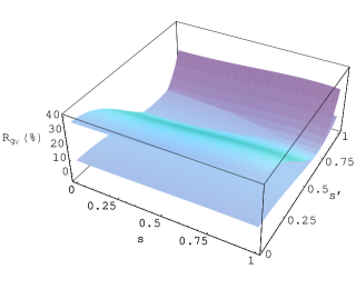
Figure 2: The relative changes $R_{g_{V}}(\%)$ and $R_{g_{A}}(\%)$ of $Z_{1}e^{+}e^{-}$ vector $g_{V}$ and axial-vector $g_{A}$ couplings from the SM values depending on $s$ and $s^{\prime}$ taking the scale $f=3$ TeV (upper on left panel, lower on right panel) and $f=6$ TeV (lower on left panel, upper on right panel).

The couplings of the $Z_{1}$ boson and $W_{1}$ boson to the SM leptons are subject to corrections in the LHM. Using their couplings shown in Table 1 one obtains for the $Z_{1}$ total decay width and $W_{1}$ boson mass up to corrections proportional to $\mathcal{O}(v^{2}/f^{2})$: $\Gamma_{Z_{1}}\simeq\Gamma_{Z}(1+1.7v^{2}/f^{2})$ and $m_{W_{1}}\simeq m_{W}(1+0.89v^{2}/f^{2})$, leading to the comment that $f>8$ TeV even for small $c^{\prime}$. Since there is some partial cancellations, in fact as a general guide we take $v/f\lesssim 0.1$. We present the decay widths of $Z_{2}$ and $W_{2}^{\pm}$ bosons which we need in the calculation of the cross section for process $e^{+}e^{-}\to\nu\bar{\nu}\gamma$. The decay of heavy gauge boson $Z_{2}$ include leptonic, hadronic and gauge boson channels to give the partial widths of the form Han03 (2)

$$\Gamma(Z_{2}\rightarrow l^{+}l^{-})\simeq\frac{g^{2}\cot^{2}\theta}{96\pi}m_{Z_{2}},\qquad\Gamma(Z_{2}\rightarrow\bar{q}q)\simeq\frac{g^{2}\cot^{2}\theta}{32\pi}m_{Z_{2}}$$

$$\Gamma(Z_{2}\rightarrow Z_{1}h)\simeq\frac{g^{2}\cot^{2}2\theta}{192\pi}m_{Z_{2}},\qquad\Gamma(Z_{2}\rightarrow W_{1}^{+}W_{1}^{-})\simeq\frac{g^{2}\cot^{2}2\theta}{192\pi}m_{Z_{2}}$$ (9)

where we neglect the corrections from the $v/f$ terms and the final state masses. The partial decay widths for the $W_{2}^{\pm}$ bosons can be obtained from (9) using the isospin symmetry, as follows

$$\Gamma(W_{2}^{\pm}\rightarrow l^{\pm}\nu)\simeq\frac{g^{2}\cot^{2}\theta}{48\pi}m_{W_{2}},\qquad\Gamma(W_{2}^{\pm}\rightarrow\bar{q}^{\prime}q)\simeq\frac{g^{2}\cot^{2}\theta}{16\pi}m_{W_{2}}$$

$$\Gamma(W_{2}^{\pm}\rightarrow W_{1}^{\pm}h)\simeq\frac{g^{2}\cot^{2}2\theta}{192\pi}m_{Z_{2}},\qquad\Gamma(W_{2}^{\pm}\rightarrow W_{1}^{\pm}Z_{1})\simeq\frac{g^{2}\cot^{2}2\theta}{192\pi}m_{Z_{2}}$$ (10)

The gauge boson $Z_{3}$ is assumed to be light and could be explored at future colliders. Similarly, its decay width can be obtained from (1) by replacing $g\to g^{\prime}$ and $\theta\to\theta^{\prime}$.

Figure 3: The Feynman diagrams contributing to the process $e^{+}e^{-}\rightarrow\nu\bar{\nu}\gamma$.

After these preliminary remarks, let we consider the process $e^{-}(p_{1})e^{+}(p_{2})\rightarrow\nu(k_{1})\bar{\nu}(k_{2})\gamma(k)$ in LHM for which relevant diagrams are presented in Fig. 3. In the SM, this process proceeds via s-channel $Z$ and t-channel $W^{\pm}$ exchange with the photon being radiated from the initial charged paticles. In the LHM models this process has also contributions from both s-channel $Z_{2},Z_{3}$ and t-channel $W_{2}^{\pm}$ exchange. We implement all relevant vertices in the CalcHEP Pukhov99 (11) in the framework of the littlest Higgs model. The amplitudes for the diagrams Fig. 3(a-c) are given by

$$M_{1} = \sum_{a=1}^{3}\bar{u}(k_{1})[-i\gamma^{\mu}(g_{V}^{a(\nu)}+g_{A}^{a(\nu)}\gamma_{5})]v(k_{2})\left[\frac{-i(g_{\mu\nu}-q_{1\mu}q_{1\nu}/m_{Z_{a}}^{2})}{q_{1}^{2}-m_{Z_{a}}^{2}+im_{Z_{a}}\Gamma_{Z_{a}}}\right]$$ (11)

$$\bar{v}(p_{2})(ig_{e}\not\varepsilon)\left[\frac{i(\not q+m_{e})}{q^{2}-m_{e}^{2}}\right](-i\gamma^{\nu})(g_{V}^{a(e)}+g_{A}^{a(e)}\gamma_{5})u(p_{1})$$

where $q_{1}=k_{1}+k_{2}$, $q=k-p_{2}$ and $\varepsilon_{\mu}$ is the photon polarisation four-vector. The amplitudes for Fig. 3(d-f) are given by

$$M_{2} = \sum_{a=1}^{3}\bar{u}(k_{1})[-i\gamma^{\mu}(g_{V}^{a(\nu)}+g_{A}^{a(\nu)}\gamma_{5})]v(k_{2})\left[\frac{-i(g_{\mu\nu}-q_{1\mu}q_{1\nu}/m_{Z_{a}}^{2})}{q_{1}^{2}-m_{Z_{a}}^{2}+im_{Z_{a}}\Gamma_{Z_{a}}}\right]$$ (12)

$$\bar{v}(p_{2})(-i\gamma^{\nu})(g_{V}^{a(e)}+g_{A}^{a(e)}\gamma_{5})\left[\frac{i(\not q^{\prime}+m)}{q^{\prime 2}-m_{e}^{2}}\right](ig_{e}\not\varepsilon)u(p_{1})$$

where $q^{\prime}=p_{1}-k$. The amplitudes for Fig. 3(g,h) are given by

$$M_{3} = \sum_{b=1}^{2}\bar{u}(k_{1})(-ig_{V}^{b}\gamma^{\mu})(1-\gamma_{5})\frac{i(\not q+m_{e})}{q^{\prime 2}-m_{e}^{2}}](ig_{e}\not\varepsilon)u(p_{1})$$ (13)

$$\left[\frac{-i(g_{\mu\nu}-q_{3\mu}q_{3\nu}/m_{W_{b}}^{2})}{q_{3}^{2}-m_{W_{b}}^{2}+im_{W_{b}}\Gamma_{W_{b}}}\right]\bar{v}(p_{2})(-ig_{V}^{b}\gamma^{\nu})(1-\gamma_{5})v(k_{2})$$

where $q_{3}=p_{2}-k_{2}$. The amplitudes for Fig. 3(i,j) are given by

$$M_{4} = \sum_{b=1}^{2}\bar{u}(k_{1})(-ig_{V}^{b}\gamma^{\mu})(1-\gamma_{5})u(p_{1})\left[\frac{-i(g_{\mu\nu}-q_{4\mu}q_{4\nu}/m_{W_{b}}^{2})}{q_{4}^{2}-m_{W_{b}}^{2}+im_{W_{b}}\Gamma_{W_{b}}}\right]$$ (14)

$$\bar{v}(p_{2})(ig_{e}\not\varepsilon)\left[\frac{i(\not q+m)}{q^{2}-m_{e}^{2}}\right](-ig_{V}^{b}\gamma^{\nu})(1-\gamma_{5})v(k_{2})$$

where $q_{4}=k_{1}-p_{1}$. The amplitudes for Fig. 3(k,l) are given by

$$M_{5} = \sum_{b=1}^{2}\bar{u}(k_{1})(-ig_{V}^{b}\gamma_{\mu})(1-\gamma_{5})u(p_{1})\left[\frac{-i(g^{\mu\mu^{\prime}}-q_{4}^{\mu}q_{4}^{\mu^{\prime}}/m_{W_{b}}^{2})}{q_{4}^{2}-m_{W_{b}}^{2}+im_{W_{b}}\Gamma_{W_{b}}}\right]$$ (15)

$$ig_{e}(g_{\nu^{\prime}\lambda}(q_{3}+k)_{\mu^{\prime}}+g_{\lambda\mu^{\prime}}(-k+q_{4})_{\nu^{\prime}}+g_{\mu^{\prime}\nu^{\prime}}(-q_{4}-q_{3})_{\lambda})\varepsilon^{\lambda}$$

$$\left[\frac{-i(g^{\nu\nu^{\prime}}-q_{3}^{\nu}q_{3}^{\nu^{\prime}}/m_{W_{b}}^{2})}{q_{3}^{2}-m_{W_{b}}^{2}+im_{W_{b}}\Gamma_{W_{b}}}\right]\bar{v}(p_{2})(-ig_{V}^{b}\gamma_{\nu})(1-\gamma_{5})v(k_{2})$$

III Numerical Results

We will interest the differential cross sections over the kinematic observables of the photon energy $E_{\gamma}$ and its angle relative to incident electron direction, respectively. The double differential cross section of the considered process is given by

$$\frac{d\sigma}{dE_{\gamma}d\cos\theta_{\gamma}}=\frac{\left|M\right|^{2}E_{\gamma}}{128\pi^{3}s}$$ (16)

where the amplitude $M$ is the sum of above five amplitudes, $M_{1-5}$. In order to remove the collinear singularities, when the photon is emitted in the initial beam direction, we apply the initial kinematic cuts: $E_{\gamma}>10$ GeV and $10^{o}<\theta_{e\gamma}<170^{o}$. We may also impose a cut, $p_{T\gamma}>10$ GeV, on the transverse momentum of photon to remove the large background from radiative Bhabba scattering. Figure 4 shows the total cross section for $e^{+}e^{-}\to\nu\bar{\nu}\gamma$ as a function of the center of mass energy $\sqrt{s}$ for the SM and two different values of the LHM parameters $s$ and $s^{\prime}$. Starting from a center of mass energy just greater than the $Z$ mass, a minimum around $\sqrt{s}\simeq 300$ GeV occurs due to the SM $Z$-boson resonance tail on the high energies. For different values of the parameters $s,s^{\prime}$ and $f$ the shape of the LHM curves changes leading to the appearence/disappearence of the resonance peaks. For the proposed energies and luminosities of the ILC and CLIC $e^{+}e^{-}$ colliders we can well measure different extra gauge boson couplings for the interested region of the parameters. In other words, preferably we may search for $Z_{3}$ at ILC ($0.5-1$ TeV) energies and $Z_{2}$ at CLIC energies ($1-5$ TeV).

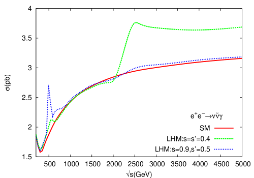
Figure 4: The total cross section in pb versus center of mass energy $\sqrt{s}$. For the LHM model we take two different points for $s,s^{\prime}$ and $v/f=0.1$.

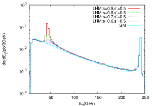
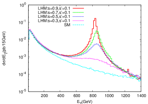
Figure 5: Diferential cross section versus photon energy at $\sqrt{s}=500$ GeV (left) and $\sqrt{s}=3000$ GeV (right) for $v/f=0.1$ and different values of $s,s^{\prime}$.

Table 2: Masses and decay widths of neutral $(Z_{2,3})$ and charged $(W_{2}^{\pm})$ gauge bosons. Here we use $v/f=0.1$ and $y_{e}=0.6$.

$\sin\theta/\sin\theta^{\prime}$	$m_{Z_{2}}$(GeV)	$m_{Z_{3}}$(GeV)	$m_{W_{2}}$(GeV)	$\Gamma_{Z_{2}}$(GeV)	$\Gamma_{Z_{3}}$(GeV)	$\Gamma_{W_{2}}$(GeV)
0.1/0.1	8034.4	1971.2	8034.4	27153.0	6614.7	26899.80
0.3/0.1	2787.0	1971.7	2792.4	960.32	693.95	953.17
0.4/0.1	2138.4	1972.7	2179.6	382.35	370.61	385.61
0.5/0.3	1843.9	684.5	1844.8	187.99	70.06	186.09
0.5/0.5	1844.5	451.7	1844.8	188.05	45.90	186.09
0.5/0.9	1844.1	499.6	1844.8	188.01	50.84	186.09
0.9/0.5	2036.2	452.6	2036.6	17.95	3.65	17.78
0.9/0.9	2036.3	498.7	2036.6	17.95	4.09	17.78

In table 3 and 4 we present the total cross section for the process $e^{+}e^{-}\to\nu\bar{\nu}\gamma$ with both signal and SM background. We find the total cross section (signal+background) changes at most $\%44$ at $\sqrt{s}=0.5$ TeV for the interested region of the parameters $s,s^{\prime}$ with the scale $f=2.46$ TeV. There is also a large contribution from extra gauge bosons, mainly $Z_{2}$, for relatively small parameter $s^{\prime}=0.1$ with a larger values of $s=0.9$ and the scale $f=3.5$ TeV at the center of mass energy $\sqrt{s}=3$ TeV as shown in table 4. In order to see sensitivity of the photon energy to new physics, in Fig. 5 we plot the differential cross section versus $E_{\gamma}$ by taking $v/f=0.1$ at the center of mass energy $\sqrt{s}=0.5$ TeV and $\sqrt{s}=3$ TeV, respectively. We see that for the value of parameter $s^{\prime}=0.5$ the $Z_{3}$ resonance occurs as its magnitude strongly depends on the values of $s$. The peak in the cross section due to $Z_{3}$ ($Z_{2}$) boson shifts to the right as $s$ decrease. We see from Figure 5 that main contributions to the total cross section (signal+background) comes from three regions, low energy region, resonance region and the region due to radiative return to the $Z$ pole, where $E_{\gamma}=\sqrt{s}(1-m_{Z}^{2}/s)/2\approx 240$ GeV. The pole region ($\sim\sqrt{s}/2$) is quite insensitive to the new physics. The resonance region for $Z_{3}$ occurs at $s^{\prime}=0.5$ and $f\simeq 1-3$ TeV. The peak of the resonance shifts to lower photon energies (left) when the scale $f$ increased as shown in Fig. 6. This is due to the fact that as $f$ increases the extra gauge boson masses ($\propto f$) also increase, as the resonance occurs there remains lower energy delivered to the photon, i.e. the lower $E_{\gamma}$, the higher the mass probed in the $Z_{i}$ propagator via $E_{\gamma}=\sqrt{s}(1-m_{Z_{i}}^{2}/s)/2$. For a visible signal peak one can scan the parameter $f$ between $\simeq 1-3$ TeV at a collider energy of $\sqrt{s}=0.5$ TeV. At higher center of mass energies such as $\sqrt{s}=3$ TeV this resonance scan can be extended to upper values of the scale $f$ around $\simeq 2-4$ TeV.

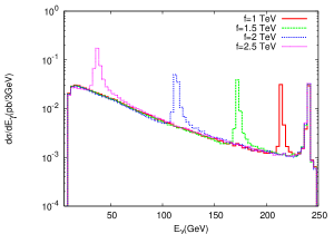
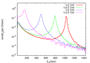
Figure 6: Energy distribution of photon for different values of the scale $f$ at $\sqrt{s}=500$GeV (left) and $\sqrt{s}=3000$ GeV (right). The sine of mixing angle is taken as $s=0.9$,$s^{\prime}=0.5$ for the left plot, and $s=0.9,s=0.1$ for the right plot.

Table 3: The cross sections (in pb) for $e^{+}e^{-}\to\nu\bar{\nu}\gamma$ with $v/f=0.1$ at $\sqrt{s}=500$ GeV. The corresponding SM background gives $\sigma_{B}=1.879$ pb. Here we applied the minimal cuts $E_{\gamma}>10$ GeV, $10^{o}<\theta_{13}<170^{o}$ and $p_{T}>10$ GeV.

$\sin\theta$\$\sin\theta^{\prime}$	0.1	0.3	0.5	0.7	0.9
0.1	1.9379	1.9347	1.9382	1.9396	1.9384
0.3	1.9662	1.9701	1.9035	1.8919	1.9041
0.5	1.9761	2.0012	1.9294	1.8806	1.9305
0.7	1.9755	1.9983	2.0394	1.8905	1.9583
0.9	1.9606	1.9915	2.7090	1.8878	1.9668

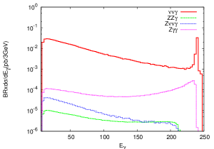
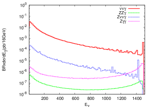
Figure 7: Backgrounds contributing to an $"\gamma+nothing"$ analysis.

Table 4: The cross sections (in pb) for $e^{+}e^{-}\to\nu\bar{\nu}\gamma$ with $v/f=0.07$ at $\sqrt{s}=3000$ GeV. The corresponding SM background gives $\sigma_{B}=3.013$ pb. Here we applied the minimal cuts $E_{\gamma}>10$ GeV, $10^{o}<\theta_{13}<170^{o}$ and $p_{T}>10$ GeV.

$\sin\theta$\$\sin\theta^{\prime}$	0.1	0.3	0.5	0.7	0.9
0.1	3.2502	3.2093	3.2206	3.2359	3.2311
0.3	4.2023	3.0384	3.0505	3.0578	3.0614
0.5	10.369	3.3954	3.4205	3.4199	3.4083
0.7	24.491	3.1316	3.1323	3.1345	3.1343
0.9	66.303	3.1130	3.0709	3.0768	3.0722

Table 5: The cross sections (in fb) for relevant background processes at ILC and CLIC energies with (w) and without (o) initial state radiation (ISR) from $e^{+}$ and $e^{-}$ beams. Here, we applied only the initial cuts.

w/o ISR	$\sigma(\nu\bar{\nu}\gamma)$	$\sigma(Z\gamma)$	$ZZ\gamma$	$Z\nu\bar{\nu}\gamma$
$\sqrt{s}=0.5$ TeV	$1843.0/1879.3$	$2273.0/1730.5$	$22.94/22.71$	$10.88/11.76$
$\sqrt{s}=1$ TeV	$2372.6/2429.5$	$582.16/416.13$	$11.96/11.20$	$35.73/39.92$
$\sqrt{s}=3$ TeV	$2970.4/3012.7$	$70.03/45.72$	$3.00/2.63$	$129.72/133.18$
$\sqrt{s}=5$ TeV	$3125.4/3152.2$	$26.43/16.44$	$1.44/1.23$	$174.81/189.04$

We calculate the relevant backgrounds from the reactions $e^{+}e^{-}\to Z\gamma$ ($2\to 2$) which is the part of $e^{+}e^{-}\to\nu\bar{\nu}\gamma$ ($2\to 3$) reaction, $e^{+}e^{-}\to ZZ\gamma$ ($2\to 3$) and $e^{+}e^{-}\to Z\nu\bar{\nu}\gamma$ ($2\to 4$) with (w) and without (o) ISR effects at the ILC and CLIC energies. With the initial cuts we find the background cross sections as shown in Table 5. We see the main contribution to the background comes from $e^{+}e^{-}\to\nu\bar{\nu}\gamma$ which includes both $e^{+}e^{-}\to Z\gamma$ ($2\to 2$) and $e^{+}e^{-}\to\nu\bar{\nu}\gamma$ ($2\to 3$ with only $W_{1}$ exchange). Here we take branching ratio of $Z^{0}\to$invisible decay as $20\%$. A background which cannot be suppressed, comes from the process $e^{+}e^{-}\to\nu\bar{\nu}\nu^{\prime}\bar{\nu^{\prime}}\gamma$ with a cross section $\sigma\backsimeq 23$ fb. In order to see the photon energy distribution (between the initial cuts and kinematical cuts) of these backgrounds in the $"\gamma+nothing"$ analysis we show differential cross sections multiplied by corresponding branching ratios in Fig. 7 at the center of mass energies $\sqrt{s}=0.5$ TeV and $\sqrt{s}=3$ TeV. Here, we assume lepton universality, and calculate the cross sections to give an idea about the magnitude of the background considered. In general, applying some strict cuts around the resonance regions and by making an optimization for $S/B$ ratio, the measurements can also be improved, provided that the LHC measures the masses of the extra gauge bosons predicted by the LHM.

For a given center of mass energy we can determine the contributions from new gauge bosons in different parameter regions: one is the resonant region where a peak in the distribution is obtained for some certain values of the parameters $s,s^{\prime}$ and $f$; second is non-resonant region where the parameter scans can be performed over a wide range; third is the decoupling region ($c^{\prime}=\sqrt{2/5}$) where the coupling of $Z_{3}$ to fermions vanishes, here there is also another approach that the mass of the new gauge boson can be taken infinitely heavy. We show the results for the mentioned cases during our analysis.

In order to obtain the discovery limits of the LHM parameters we perform the $\chi^{2}$ analysis. We calculate the $\chi^{2}$ distribution as

$$\chi^{2}={\displaystyle\sum_{k=1}^{n}\left(\frac{\frac{d\sigma^{k}}{dE_{\gamma}}(\mbox{LHM})-\frac{d\sigma^{k}}{dE_{\gamma}}(\mbox{SM})}{\delta\frac{d\sigma^{k}}{dE_{\gamma}}(\mbox{SM})}\right)^{2}}$$ (17)

where $\delta d\sigma^{k}/dE_{\gamma}$ is the error on the measurement including statistical and systematical errors added in quadrature. As we already noted that the backgrounds are much smaller than the signal, we expect the statistical errors in the SM backgrounds would be smaller than the systematic errors including detector and $e^{-}/e^{+}$ beam uncertainties. Here, we considered a systematic error $\delta_{sys}=5\%$ for a measurement. This may be an overestimate, however, if improved the constraints can be relaxed and benefit from the advantage of high luminosity. The differential cross section depends on the model parameters $s,s^{\prime}$ and $f$. We may assume that the LHC would have determined the mass of the extra gauge bosons relatively well, to the order of a few percent. Thus we can fix $m_{Z_{i}}$and perform a two-parameter scan. We calculate $\chi^{2}$ at every point of $s,s^{\prime}$. In this case $\chi^{2}=\chi_{\min}^{2}+C$. The constraint on the parameters with $95\%$ C.L. can be obtained at the ILC and CLIC energies by requiring $C=5.99$ for two free parameters. In calculating the $\chi^{2}$ for $d\sigma/dE_{\gamma}$we have used equal sized bins in the range $E_{\gamma}^{min}<E_{\gamma}<E_{\gamma}^{max}$ where the upper limit is taken as the kinematical limit for the photon energy. The most sensitive results can be obtained for $s^{\prime}=0.5(0.1)$ at the center of mass energy $\sqrt{s}=0.5(3)$ TeV as shown in Fig. 8. The $\chi_{i}^{2}$ distributions versus the photon energy bins show peaks shifted to the right depending on lower $s$ and lower $f$ values. Here we have used $v/f=0.1$ and $0.07$ for the ILC and CLIC energies, respectively.

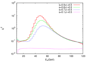
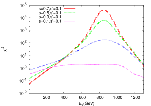
Figure 8: The $\chi_{i}^{2}$ distribution depending on the energy bins $i$ for different LHM mixing parameters at ILC with $\sqrt{s}=500$GeV (left) and CLIC with $\sqrt{s}=3$ TeV (right) , here we assume $L_{int}=100$ fb^-1 and $v/f=0.1$.

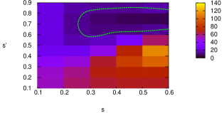
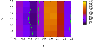
Figure 9: The density plot and the contour lines with $95\%$ C.L. for the search reach in the parameter space ($s,s^{\prime}$) with $v/f=0.1$ (left) and $v/f=0.07$ (right) at ILC (left) and CLIC (right) energies.

In Fig. 9 we present the constraints on mixing parameters $s,s^{\prime}$ in a density plot. For the $Z_{3}$ search at the ILC energies with $L_{int}=100$ fb^-1 most of the $s,s^{\prime}$ parameter space can be discoverd. A contour line for the constrained parameter space ($s,s^{\prime}$) is also shown on the plot. We may exclude the region with $0.6<s^{\prime}<0.8$, $0.25<s<0.9$ by this analysis at $\sqrt{s}=0.5$ TeV. When the systematic error is not included, the shape of the plot is luminosity dependent, even for a low luminosity as $L_{int}\sim 10^{3}$ pb^-1 only the decoupling region ($s^{\prime}=\sqrt{3/5}$) remains dark (not accessible) in this plot. At higher center of mass energies different parameter regions can be constrained. The resonance regions deserve special attention at the ILC and CLIC energies. Because the highest sensitivity to new physics is obtained in this region. Taking $s^{\prime}=0.5$ we can probe the $Z_{3}$ signal for the interested range of $s=0.5-0.9$ and $f=0.5-2.7$ TeV at $\sqrt{s}=0.5$ TeV and $L_{int}=100$ fb^-1 . For the CLIC at $\sqrt{s}=3$ TeV and $L_{int}=100$ fb^-1, and taking the mixing parameter $s^{\prime}=0.1$, we can probe the resonance peaks between the scale $f=1-3.7$ TeV for almost all range of $s$. The extra gauge boson signals of LHM can be measured for almost all interested range of $s,s^{\prime}$ except $0.3<s<0.4$ at CLIC with a projected luminosity $L_{int}=100$ fb${}^{-1}.$

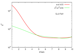
Figure 10: The $\chi^{2}$ plot (left), and total cross sections for the LHM signal and SM background (right) versus the scale $f$ for fixed values of the parameters $s,s^{\prime}=0.5$ and $s,s^{\prime}=\sqrt{3/5}$ at CLIC with $\sqrt{s}=3$ TeV, $L_{int}=100$ fb^-1.

We continue our analysis with higher values of the scale $f$ as $f\gtrsim 4$ TeV, and we would like to determine the accuracy of the parameter measurements using a $\chi^{2}$ analysis. The best discovery limit is obtained using the observable $d\sigma/dE_{\gamma}$. We calculate the $\chi_{\min}^{2}$, and determine the discovery region corresponding to $\chi^{2}<\chi_{\min}^{2}+2.69$ for one free parameter. As the references we take the parameters $s,s^{\prime}=1/2$ and $s,s^{\prime}=\sqrt{3/5}$, first is arbitrary but the latter corresponds to decoupling the $Z_{3}$ from the leptonic current. If the masses of extra gauge bosons can not be measured at the LHC, we may need to scan parameter $f$ at higher energies. In Fig. 10, for the CLIC energies we depict the $\chi^{2}$ plot versus the scale $f$ for fixed values of $s$ and $s^{\prime}$. We also show the signal and background cross sections versus $f$. Based on the analysis mentioned above, the parameter $f$ can be reached up to 6 TeV at CLIC with $\sqrt{s}=3$ TeV. We can measure the scale $f$ (or the mass of heavy gauge boson) with an error of $5\%$. This limit enhances when we take into account smaller systematic errors for a measurement.

IV Conclusions

In this work, we have studied the sensitivity of the process $e^{+}e^{-}\to\nu\bar{\nu}\gamma$ to the extra gauge bosons $Z_{2},Z_{3}$ and $W_{2}^{\pm}$ in the framework of the little Higgs model. The search reach of the ILC (operating at $\sqrt{s}=0.5$ TeV and $L_{int}=100$ fb^-1 for one year) and CLIC (when operating at $\sqrt{s}=3$ TeV, and $L_{int}=100$ fb^-1) covers a wide range of parameter space where this model relevant to the hierarchy. For the parameter space where the resonances occur ($s^{\prime}=0.5(0.1)$) by scanning the parameter $s$, we can access the range for scale $f=0.5-2.7$ ($1-3.7$) TeV at $\sqrt{s}=0.5$ ($3$) TeV, respectively. If the scale $f$ is larger than $f\gtrsim 4$ TeV, a sensitivity to the parameters of LHM could be reached with a detailed MC including detector and beam luminosity/energy uncertainty effects.

Finally, the ILC and CLIC with high luminosity have a high search potential for different regions of parameter space of the LHM. Analysis of $e^{+}e^{-}\to\nu\bar{\nu}\gamma$ process can give valuable information about the LHM and it can serve a clean environment for precise determination its parameters. The measurements with small systematic errors are needed to have desired sensitivity for the new physics parameters. Even for the cases in which search reach for extra gauge bosons in this process is not competitive with the potential of the LHC, the measurements at linear colliders can also provide detailed information on extra gauge bosons which complements the results from the LHC.

References

(1)N. Arkani-Hamed et al., JHEP 07 (2002) 034; N. Arkani-Hamed
et al., JHEP 08 (2002) 021.
(2)T. Han et al., Phys. Rev. D 67 (2003) 095004; M. Schmaltz
and D.T. Smith, Ann. Rev. Nucl. Part. Sci. 55, (2005) 229;
M. Perelstein, Prog. Part. Nucl. Phys. 58 (2007) 247.
(3)C. Csaki et al., Phys. Rev. D 67 (2003) 115002; J.L. Hewett,
F.J. Petriello and T.G. Rizzo, JHEP 0310 (2003) 062; M.C.
Chen and S. Dawson, Phys. Rev. D 70 (2004) 015003; C.x. Yue
and W. Wang, Nucl. Phys. B 683 (2004) 48; W. Kilian and J.
Reuter, Phys. Rev. D 70 (2004) 015004; T. Han et al., Phys.
Lett. B 563 (2003) 191.
(4)M. Blanke et al., hep-ph/0704.3329; hep-ph/0703254; M. Blanke
and A.J. Buras, hep-ph/0703117; M. Blanke et al., JHEP 0701
(2007) 066; M. Blanke et al., JHEP 0612 (2006)003.
(5)P. Kai et al., hep-ph/07061358; X. Wang et al., hep-ph/0702164;
F.M.L. de Almeida et al., hep-ph/0702137; X. Wang et
al., hep-ph/0702064.
(6)J.A. Conley, J. Hewett and M.P. Le, Phys. Rev. D 72, (2005)
115014.
(7)G. Azuelos et al., Eur. Phys. J. C. 3952 (2005) 13.
(8)R. Brinkmann et al., TESLA technical design report,
DESY-2001-011, 2001; G.A. Loew, Report from the International Linear
Collider Technical Review Committee, SLAC-PUB-10024, 2003; A
comprehensive information about the future linear colliders can be
found at the URL: http://www.linearcollider.org.
(9)R.W. Assmann et al., The CLIC Study Team, A 3 TeV
linear collider based on CLIC technology, CERN 2000-008, Geneva,
2000; R.W. Assmann et al., The CLIC Study Team, CLIC
contribution to the technical review committee on a 500 GeV
linear collider, CERN-2003-007, Geneva, 2003; E. Accomando et
al., Report of the CLIC physics working group, CERN-2004-005,
Geneva, 2004; hep-ph/0412251.
(10)E. Ma and J. Okada, Phys. Rev. D 8 (1978) 4219.
(11)A. Pukhov et al., CalcHEP/CompHEP Collab., hep-ph/9908288 ;
hep-ph/0412191.