Channel Capacity Estimation using Free Probability Theory

Abstract

In many channel measurement applications, one needs to estimate some characteristics of the channels based on a limited set of measurements. This is mainly due to the highly time varying characteristics of the channel. In this contribution, it will be shown how free probability can be used for channel capacity estimation in MIMO systems. Free probability has already been applied in various application fields such as digital communications, nuclear physics and mathematical finance, and has been shown to be an invaluable tool for describing the asymptotic behaviour of many large-dimensional systems. In particular, using the concept of free deconvolution, we provide an asymptotically (w.r.t. the number of observations) unbiased capacity estimator for MIMO channels impaired with noise called the free probability based estimator. Another estimator, called the Gaussian matrix mean based estimator, is also introduced by slightly modifying the free probability based estimator. This estimator is shown to give unbiased estimation of the moments of the channel matrix for any number of observations. Also, the estimator has this property when we extend to MIMO channels with phase off-set and frequency drift, for which no estimator has been provided so far in the literature. It is also shown that both the free probability based and the Gaussian matrix mean based estimator are asymptotically unbiased capacity estimators as the number of transmit antennas go to infinity, regardless of whether phase off-set and frequency drift are present. The limitations in the two estimators are also explained. Simulations are run to assess the performance of the estimators for a low number of antennas and samples to confirm the usefulness of the asymptotic results.

I Introduction

Random matrices, and in particular limit distributions of sample covariance matrices, have proved to be a useful tool for modelling systems, for instance in digital communications [1], nuclear physics [2] and mathematical finance [3]. A typical random matrix model is the information-plus-noise model,

$${\bf W}_{n}=\frac{1}{N}({\bf R}_{n}+\sigma{\bf X}_{n})({\bf R}_{n}+\sigma{\bf X}_{n})^{H}.$$ (1)

${\bf R}_{n}$ and ${\bf X}_{n}$ are assumed independent random matrices of dimension $n\times N$, where ${\bf X}_{n}$ contains i.i.d. standard (i.e. mean $0$, variance $1$) complex Gaussian entries. (1) can be thought of as the sample covariance matrices of random vectors ${\bf r}_{n}+\sigma{\bf x}_{n}$. ${\bf r}_{n}$ can be interpreted as a vector containing the system characteristics (direction of arrival for instance in radar applications or impulse response in channel estimation applications). ${\bf x}_{n}$ represents additive noise, with $\sigma$ a measure of the strength of the noise. Classical signal processing estimation methods consider the case where the number of observations $N$ is highly bigger than the dimensions of the system $n$, for which equation (1) can be shown to be approximately:

$${\bf W}_{n}={\bf\Gamma}_{n}+\sigma^{2}{\bf I}_{n}.$$ (2)

Here, ${\bf\Gamma}_{n}$ is the true covariance of the signal. In this case, one can separate the signal eigenvalues from the noise ones and infer (based only on the statistics of the signal) on the characteristics of the input signal. However, in many situations, one can gather only a limited number of observations during which the characteristics of the signal does not change. In order to model this case, $n$ and $N$ will be increased so that $\lim_{n\rightarrow\infty}\frac{n}{N}=c$, i.e. the number of observations is increased at the same rate as the number of parameters of the system (note that equation (2) corresponds to the case $c=0$).

Previous contributions have already dealt with this problem. In [4], Dozier and Silverstein explain how one can use the eigenvalue distribution of ${\bf\Gamma}_{n}=\frac{1}{N}{\bf R}_{n}{\bf R}_{n}^{H}$ to estimate the eigenvalue distribution of ${\bf W}_{n}$ by solving a given equation. In [5, 6], we provided an algorithm for passing between the two, using the concept of multiplicative free convolution, which admits a convenient implementation. The implementation performs free convolution exactly based solely on moments.

In this paper, channel capacity estimation in MIMO systems is used as a benchmark application by using the connection between free probability theory and systems of type (1). For MIMO channels with and without frequency off-sets, we derive explicit asymptotically unbiased estimators which perform much better than classical ones. We do not prove directly that the proposed estimators work better than the classical ones, but present simulations which indicate that they are superior. We remark that the proposed capacity estimators will not be unbiased, it is needed that either the number of transmit antennas or the number of observations be large to obtain precise estimation. This limitation is most severe for channels with frequency off-sets, where it is needed in any case that the number of transmit antennas is large to obtain precise estimation. A case of study where channel estimation using free deconvolution has been used can be found in [7] and [8].

This paper is organized as follows. Section II presents the problem under consideration. Section III provides the basic concepts needed on free probability, including free convolution. In section IV, we formalize a new channel capacity estimator based on free probability, and explain some of the shortcomings for MIMO models with frequency off-sets. Another estimator, called the Gaussian matrix mean based estimator is then formalized to address the shortcomings of the free probability based estimator. We also present arguments for the Gaussian matrix mean based estimator performing better than the free probability based estimator, in some specific cases. These arguments are, however, not definite; we do not prove that one estimator is better than the other for the cases considered. The limitations of the estimators are also explained. The low rank of the channel (less than or equal to four) is the most notable limitation. In section V, simulations of the estimators are performed and compared, where several quantities are varied, like the noise variance, rank and dimensions of the channel matrix, and the number of observations. In the following, upper (lower boldface) symbols will be used for matrices (column vectors) whereas lower symbols will represent scalar values, $(.)^{T}$ will denote transpose operator, $(.)^{\star}$ conjugation and $(.)^{H}=\left((.)^{T}\right)^{\star}$ hermitian transpose. ${\bf I}_{n}$ will represent the $n\times n$ identity matrix. $Tr_{n}$ will denote the non-normalized trace on $n\times n$ matrices, while $tr_{n}=\frac{1}{n}Tr_{n}$ denotes the normalized trace. Also, we will throughout the paper use $c$ as a shorthand notation for the ratio between the number of rows and the number of columns in the random matrix model being considered.

II Statement of the problem

In usual time varying measurement methods for MIMO systems, one validates models [9] by determining how the model fits with actual capacity measurements. In this setting, one has to be extremely cautious about the measurement noise, especially for far field measurements where the signal strength can be lower than the noise.

The MIMO measured channel in the frequency domain can be modelled by [10, 11]

$$\hat{{\bf H}}_{i}={\bf D}_{i}^{r}{\bf H}{\bf D}_{i}^{t}+\sigma{\bf X}_{i}$$ (3)

where $\hat{\bf H}_{i}$, ${\bf H}$ and ${\bf X}_{i}$ are respectively the $n\times m$ measured MIMO matrix ($n$ is the number of receiving antennas, $m$ is the number of transmitting antennas), the $n\times m$ MIMO channel and the $n\times m$ noise matrix with i.i.d. standard Gaussian entries. Note that we suppose the noise matrix ${\bf X}_{i}$ to be spatially white. In the realm of the channel measurements under study, the antenna outputs are connected to different RF (Radio Frequency) chains. As a consequence, for the case under study, the channel noise impairments are independent from one received antenna to the other. When one RF chain is used, the noise to be considered is not white. This case can also be studied within the framework of free deconvolution but goes beyond the scope of the paper. We suppose that the channel ${\bf H}$, although time varying, stays constant (block fading assumption) during $L$ blocks. ${\bf D}_{i}^{r}$ and ${\bf D}_{i}^{t}$ are $n\times n$ and $m\times m$ diagonal matrices which represent phase off-sets and phase drifts (which are impairments due to the antennas and not the channel) at the receiver and transmitter given respectively by (these are supposed to vary on a block basis)

$${\bf D}_{i}^{r} = \mathrm{diag}[e^{j\phi_{1}^{i}},...,e^{j\phi_{n}^{i}}]\mbox{, and}$$

$${\bf D}_{i}^{t} = \mathrm{diag}[e^{j\theta_{1}^{i}},...,e^{j\theta_{m}^{t}}]$$

where the phases $\phi_{j}^{i}$ and $\theta_{j}^{i}$ are random. We assume all phases independent and uniformly distributed.

We will also compare (3) with the simpler model

$$\hat{{\bf H}}_{i}={\bf H}+\sigma{\bf X}_{i},$$ (4)

which is (3) without phase off-sets and phase drifts.

The capacity per receiving antenna (in the case where the noise is spatially white additive Gaussian and the channel is not known at the transmitter) of a channel with channel matrix ${\bf H}$ and signal to noise ratio $\rho=\frac{1}{\sigma^{2}}$ is given by

$$C=\frac{1}{n}\log_{2}\det\left({\bf I}_{n}+\frac{1}{m\sigma^{2}}{\bf H}{\bf H}^{H}\right)=\frac{1}{n}\sum_{l=1}^{n}\log_{2}(1+\frac{1}{\sigma^{2}}\lambda_{l})$$ (5)

where $\lambda_{l}$ are the eigenvalues of $\frac{1}{m}{\bf H}{\bf H}^{H}$. The problem consists therefore of estimating the eigenvalues of $\frac{1}{m}{\bf H}{\bf H}^{H}$ based on few observations $\hat{\bf H}_{i}$, which is paramount for modelling purposes. Note that the capacity expression supposes that the channel is perfectly known at the receiver and not at the transmitter. In practice, with the noise impairment, the channel will never be estimated perfectly and therefore expression (5) is not achievable. However, for MIMO modelling purposes, for which the capacity is often the matching metric, one needs to compare the capacity of the model with expression (5).

There are different methods actually used for channel capacity estimation [12, 13, 14, 15]. Usual methods discard, through an ad-hoc threshold procedure, all channels $\hat{\bf H}_{i}$ for which the channel to noise ratio ($\frac{1}{\sigma^{2}}tr_{n}({\bf H}{\bf H}^{H})$) is lower than a threshold and then compute

$$\tilde{C}(\sigma^{2})=\frac{1}{n}\log_{2}\det\left({\bf I}_{n}+\frac{1}{m\sigma^{2}}(\frac{1}{M}\sum_{i=1}^{M}\hat{{\bf H}}_{i})(\frac{1}{M}\sum_{i=1}^{M}\hat{{\bf H}}_{i})^{H})\right)$$

where $M\leq L$ is the number of channels having a signal to noise ratio higher than the threshold. One of the drawbacks of this method is that one will not analyze the true capacity but only the capacity of the ”good channels”. Moreover, one has to limit the channel measurement campaign (in order to have enough channels higher than the threshold) only to regions which are close (in terms of actual distance) enough to the base station.

Other methods, in order to have a capacity estimation at a given signal to noise ratio (different from the measured one with noise variance $\sigma^{2}$), normalize each channel realization $\hat{\bf H}_{i}$ and then compute for a different value of the noise variance $\sigma_{1}^{2}$ (for example $10dB$) the capacity estimate $\tilde{C}(\sigma_{1}^{2})$. In the case where $\sigma^{2}$ is high and $\sigma_{1}^{2}$ is low, one usually finds a high capacity estimate as one measures only the noise, which is known to have a high multiplexing gain.

In this contribution, we will provide a neat framework, based on free deconvolution, for channel capacity estimation that circumvents all the previous drawbacks. Moreover, we will deal with model (3), for which no solution has been provided in the literature so far.

III Framework for free convolution

Free probability [16] theory has grown into an entire field of research through the pioneering work of Voiculescu in the 1980’s. Free probability introduces an analogy to the concept of independence from classical probability, which can be used for non-commutative random variables like matrices. These more general random variables are elements in what is called a noncommutative probability space. This can be defined by a pair $(A,\phi)$, where $A$ is a unital $\ast$-algebra with unit $I$, and $\phi$ is a normalized (i.e. $\phi(I)=1$) linear functional on $A$. The elements of $A$ are called random variables. In all our examples, $A$ will consist of $n\times n$ matrices or random matrices. For matrices, $\phi$ will be $tr_{n}$. The unit in these $\ast$-algebras is the $n\times n$ identity matrix ${\bf I}_{n}$. The analogy to independence is called freeness:

Definition 1

A family of unital $\ast$-subalgebras $(A_{i})_{i\in I}$ will be called a free family if

$$\left\{\begin{matrix}a_{j}\in A_{i_{j}}\\ i_{1}\neq i_{2},i_{2}\neq i_{3},\cdots,i_{n-1}\neq i_{n}\\ \phi(a_{1})=\phi(a_{2})=\cdots=\phi(a_{n})=0\end{matrix}\right\}\Rightarrow\phi(a_{1}\cdots a_{n})=0.$$ (6)

A family of random variables $a_{i}$ are said to be free if the algebras they generate form a free family.

When restricting $A$ to spaces such as matrices, or functions with bounded support, it is clear that the moments of $a$ uniquely identify a probability measure, here called $\nu_{a}$, such that $\phi(a^{k})=\int x^{k}d\nu_{a}(x)$. In such spaces, the distributions of $a_{1}+a_{2}$ and $a_{1}a_{2}$ give us two new probability measures, which depend only on the probability measures associated with $a_{1}$, $a_{2}$ when these are free. Therefore we can define two operations on the set of probability measures: Additive free convolution $\eta_{1}\boxplus\eta_{2}$ for the sum of free random variables, and multiplicative free convolution $\eta_{1}\boxtimes\eta_{2}$ for the product of free random variables. These operations can in many cases be used to predict the spectrum of sums or products of large random matrices: If $a_{1n}$ has an eigenvalue distribution which approaches $\eta_{1}$ and $a_{2n}$ has an eigenvalue distribution which approaches $\eta_{2}$, then in many cases the eigenvalue distribution of $a_{1n}+a_{2n}$ approaches $\eta_{1}\boxplus\eta_{2}$.

One important probability measure is the Marc̆henko Pastur law $\mu_{c}$ [17], which has the density

$$f^{\mu_{c}}(x)=(1-\frac{1}{c})^{+}\delta_{0}(x)+\frac{\sqrt{(x-a)^{+}(b-x)^{+}}}{2\pi cx},$$ (7)

where $(z)^{+}=\mbox{max}(0,z)$, $a=(1-\sqrt{c})^{2}$, $b=(1+\sqrt{c})^{2}$, and $\delta_{0}(x)$ is dirac measure (point mass) at $0$. According to the notation in [18], $\mu_{c}$ is also the free Poisson distribution with rate $\frac{1}{c}$ and jump size $c$. We will need the following formulas for the first moments of the Marc̆henko Pastur law:

$$\begin{array}[]{lll}\int xf^{\mu_{c}}(x)dx&=&1\\ \int x^{2}f^{\mu_{c}}(x)dx&=&c+1\\ \int x^{3}f^{\mu_{c}}(x)dx&=&c^{2}+3c+1\\ \int x^{4}f^{\mu_{c}}(x)dx&=&c^{3}+6c^{2}+6c+1.\end{array}$$ (8)

(8) follows immediately from applying what is called the moment-cumulant formula [18], to the free cumulants [18] of the Marc̆henko Pastur law $\mu_{c}$. The (free) cumulants of the Marc̆henko Pastur law are $1,c,c^{2},c^{3},...$ [5]. Cumulants and the moment-cumulant formula in free probability have analogous concepts in classical probability.

$\mu_{c}$ describes asymptotic eigenvalue distributions of Wishart matrices, i.e. matrices on the form $\frac{1}{N}{\bf R}{\bf R}^{H}$, with ${\bf R}$ an $n\times N$ random matrix with independent standard complex Gaussian entries, and $\frac{n}{N}\rightarrow c$. This can be seen from the following result, where the difference from (8) vanishes when $N\rightarrow\infty$:

Proposition 1

Let ${\bf X}_{n}$ be a complex standard Gaussian $n\times N$ matrix, and set $c=\frac{n}{N}$. Then

$$\begin{array}[]{lll}E\left[tr_{n}\left(\frac{1}{N}{\bf X}_{n}{\bf X}_{n}^{H}\right)\right]&=&1\\ E\left[tr_{n}\left(\left(\frac{1}{N}{\bf X}_{n}{\bf X}_{n}^{H}\right)^{2}\right)\right]&=&c+1\\ E\left[tr_{n}\left(\left(\frac{1}{N}{\bf X}_{n}{\bf X}_{n}^{H}\right)^{3}\right)\right]&=&c^{2}+3c+1+\frac{1}{N^{2}}\\ E\left[tr_{n}\left(\left(\frac{1}{N}{\bf X}_{n}{\bf X}_{n}^{H}\right)^{4}\right)\right]&=&c^{3}+6c^{2}+6c+1+\frac{5(1+c)}{N^{2}}.\end{array}$$ (9)

This will be useful later on when we compute mixed moments of Gaussian and deterministic matrices. The proof of proposition 1 is given in appendix B.

We will also find it useful to introduce the concept of multiplicative free deconvolution: Given probability measures $\eta$ and $\eta_{2}$. When there is a unique probability measure $\eta_{1}$ such that $\eta=\eta_{1}\boxtimes\eta_{2}$, we will write $\eta_{1}=\eta\begin{picture}(9.0,5.0)\put(2.0,0.0){\framebox(5.0,5.0)[]{$\smallsetminus$}} \end{picture}\eta_{2}$, and say that $\eta_{1}$ is the multiplicative free deconvolution of $\eta$ with $\eta_{2}$. There is no reason why a probability measure should have a unique deconvolution, and whether one exists at all depends highly on the probability measure $\eta_{2}$ which we deconvolve with. This will not be a problem for our purposes: First of all, we will only have need for multiplicative free deconvolution with $\mu_{c}$, and only in order to find the moments of the channel matrix. The problem of a unique deconvolution is therefore addressed by an existing algorithm for free deconvolution [6], which finds unique moments of $\eta\begin{picture}(9.0,5.0)\put(2.0,0.0){\framebox(5.0,5.0)[]{$\smallsetminus$}} \end{picture}\mu_{c}$ (as long as the first moments of $\eta$ is nonzero).

We will need the following definitions:

Definition 2

By the empirical eigenvalue distribution of an $n\times n$ random matrix ${\bf X}$ we mean the random atomic measure

$$\frac{1}{n}\left(\delta_{\lambda_{1}({\bf X})}+\cdots+\delta_{\lambda_{n}({\bf X})}\right),$$

where $\lambda_{1}({\bf X}),...,\lambda_{n}({\bf X})$ are the (random) eigenvalues of ${\bf X}$.

Definition 3

A sequence of random variables $a_{n1},a_{n2},...$ in probability spaces $(A_{n},\phi_{n})$ is said to converge in distribution if, for any $m_{1},...,m_{r}\in\mathbb{N}$, $k_{1},...,k_{r}\in\{1,2,...\}$, we have that the limit $\phi_{n}(a_{nk_{1}}^{m_{1}}\cdots a_{nk_{r}}^{m_{r}})$ exists as $n\rightarrow\infty$.

To make the connection between models (4), (3) and model (1), we need the following result [5]:

Theorem 1

Assume that the empirical eigenvalue distribution of ${\bf\Gamma}_{n}=\frac{1}{N}{\bf R}_{n}{\bf R}_{n}^{H}$ converges in distribution almost surely to a compactly supported probability measure $\eta_{\Gamma}$. Then we have that the empirical eigenvalue distribution of ${\bf W}_{n}$ also converges in distribution almost surely to a compactly supported probability measure $\eta_{W}$ uniquely identified by

$$\eta_{W}\begin{picture}(9.0,5.0)\put(2.0,0.0){\framebox(5.0,5.0)[]{$\smallsetminus$}} \end{picture}\mu_{c}=(\eta_{\Gamma}\begin{picture}(9.0,5.0)\put(2.0,0.0){\framebox(5.0,5.0)[]{$\smallsetminus$}} \end{picture}\mu_{c})\boxplus\delta_{\sigma^{2}},$$ (10)

where $\delta_{\sigma^{2}}$ is dirac measure (point mass) at $\sigma^{2}$.

Theorem 1 can also be re-stated (through deconvolution) as

$$\eta_{W}=\left((\eta_{\Gamma}\begin{picture}(9.0,5.0)\put(2.0,0.0){\framebox(5.0,5.0)[]{$\smallsetminus$}} \end{picture}\mu_{c})\boxplus\delta_{\sigma^{2}}\right)\boxtimes\mu_{c}.$$

When we have $L$ observations $\hat{\bf H}_{i}$ in a MIMO system as in (4) or (3), we will form the $n\times mL$ random matrices

$$\hat{{\bf H}}_{1...L}={\bf H}_{1...L}+\frac{\sigma}{\sqrt{L}}{\bf X}_{1...L}$$ (11)

with

$$\hat{{\bf H}}_{1...L}=\frac{1}{\sqrt{L}}\left[\hat{{\bf H}}_{1},\hat{{\bf H}}_{2},...,\hat{{\bf H}}_{L}\right],$$

$${\bf H}_{1...L}=\frac{1}{\sqrt{L}}\left[{\bf D}_{i}^{r}{\bf H}{\bf D}_{i}^{t},{\bf D}_{i}^{r}{\bf H}{\bf D}_{i}^{t},...,{\bf D}_{i}^{r}{\bf H}{\bf D}_{i}^{t}\right],$$

$${\bf X}_{1...L}=\left[{\bf X}_{1},{\bf X}_{2},...,{\bf X}_{L}\right].$$

This is the way we will stack the observations in this paper. It is only one of many possible stackings. A stacking where the ratio between the number of rows and the number of columns converges to a quantity between $0$ and $1$ would allow us to use theorem 1 (which implicitly assumes $0<c<1$) directly to conclude almost sure convergence, which again would help us to conclude that the introduced capacity estimators are asymptotically unbiased. Such a stacking can also reduce the variance of the estimators. Even though the stacking considered here may not give the lowest variance, and may not give almost sure convergence, we show that its variance converges to $0$ and provides asymptotic unbiasedness for the corresponding capacity estimator.

For the case $L=1$, the formula

$$tr_{n}\left(\left({\bf D}_{1}^{r}{\bf H}{\bf D}_{1}^{t}\left({\bf D}_{1}^{r}{\bf H}{\bf D}_{1}^{t}\right)^{H}\right)^{j}\right)=tr_{n}\left(\left({\bf H}{\bf H}^{H}\right)^{j}\right)$$ (12)

can be combined with theorem 1 to give the approximation

$$\nu_{\frac{1}{m}\hat{\bf H}_{1}\hat{\bf H}_{1}^{H}}\begin{picture}(9.0,5.0)\put(2.0,0.0){\framebox(5.0,5.0)[]{$\smallsetminus$}} \end{picture}\mu_{\frac{n}{m}}\approx\left(\nu_{\frac{1}{m}{\bf H}{\bf H}^{H}}\begin{picture}(9.0,5.0)\put(2.0,0.0){\framebox(5.0,5.0)[]{$\smallsetminus$}} \end{picture}\mu_{\frac{n}{m}}\right)\boxplus\delta_{\sigma^{2}}.$$ (13)

for a single observation. This approximation works well when $n$ is large. For many observations, note that ${\bf H}_{1...L}{\bf H}_{1...L}^{H}={\bf H}{\bf H}^{H}$ when there is no phase off-set and phase drift, so that the approximation

$$\nu_{\frac{1}{m}\hat{\bf H}_{1...L}\hat{\bf H}_{1...L}^{H}}\begin{picture}(9.0,5.0)\put(2.0,0.0){\framebox(5.0,5.0)[]{$\smallsetminus$}} \end{picture}\mu_{\frac{n}{mL}}\approx\left(\nu_{\frac{1}{m}{\bf H}{\bf H}^{H}}\begin{picture}(9.0,5.0)\put(2.0,0.0){\framebox(5.0,5.0)[]{$\smallsetminus$}} \end{picture}\mu_{\frac{n}{mL}}\right)\boxplus\delta_{\sigma^{2}}$$ (14)

applies and generalizes (13). The ratio between the number of rows and columns in the matrices ${\bf H}_{1...L},{\bf X}_{1...L}$ and $\hat{\bf H}_{1...L}$ is $c=\frac{n}{mL}$, considering the horizontal stacking of the observations in a larger matrix. It is only this stacking which will be considered in this paper.

When phase off-set and phase drift are added, it is much harder to adapt theorem 1 to produce the moments of $\frac{1}{m}{\bf H}{\bf H}^{H}$. The reason is that theorem 1 really helps us to find the moments of $\frac{1}{m}{\bf H}_{1...L}{\bf H}_{1...L}^{H}$. In the case without phase off-set and phase drift, this is enough since these moments are equal to the moments of $\frac{1}{m}{\bf H}{\bf H}^{H}$. However, equality between these moments does not hold when phase off-set and phase drift are added. A procedure for converting between these moments may exist, but seems to be rather complex, and will not be dealt with here. In section IV, we will instead define an estimator for the channel capacity which does not stack observations into the matrix ${\bf H}_{1...L}$ at all. Instead, an estimation will be performed for each observation, taking the mean of all the estimates at the end.

IV New estimators for channel capacity

In this section, two new channel capacity estimators are defined. First, a free probability based estimator is introduced, which (for model (4)) will be shown to be asymptotically unbiased w.r.t. the number of observations. Then, by slightly modifying the free probability based estimator, we will construct what we call the Gaussian matrix mean based capacity estimator. This estimator will be shown, for model (4) and (3), to give unbiased estimates of the moments of the channel matrix for any number of observations. The computational complexity for the two estimators lies in the computation of eigenvalues and moments of the matrix ${\bf H}{\bf H}^{H}$, in addition to computing the free (de)convolution in terms of moments. For the matrix ranks considered here, free (de)convolution requires few computations. The complexity in the computation of eigenvalues and moments of the matrix ${\bf H}{\bf H}^{H}$ grows with $n$ (the number of receiving antennas), which is small in this paper. The computational complexity in the estimators grows slowly with the number of observations, since the dimensions of $\hat{\bf H}_{1...L}\hat{\bf H}_{1...L}^{H}$ does not grow with $L$.

The two estimators are stated as estimators for the lower order moments of $\frac{1}{m}{\bf H}{\bf H}^{H}$. Under the assumption that this matrix has limited rank (such as $\leq 4$ here), estimators for lower order moments can be used to define estimators for the channel capacity, since the capacity can be written as a function of the $r$ lowest moments when the matrix has rank $r$, as explained below.

IV-A The free probability based capacity estimator

The free probability based estimator is defined as follows:

Definition 4

The free probability based estimator for the capacity of a channel with channel matrix ${\bf H}$ of rank $r$, denoted $C_{f}$, is computed through the following steps:

1. Compute the first $r$ moments $\hat{h}_{1},...,\hat{h}_{r}$ of the sample covariance matrix $\frac{1}{m}\hat{\bf H}_{1...L}\hat{\bf H}_{1...L}^{H}$ (i.e. compute $\hat{h}_{j}=tr_{n}\left(\left(\frac{1}{m}\hat{\bf H}_{1...L}\hat{\bf H}_{1...L}^{H}\right)^{j}\right)$ for $1\leq j\leq r$),

2. use (14) to estimate the first $r$ moments $h_{f1},...,h_{fr}$ of $\frac{1}{m}{\bf H}{\bf H}^{H}$,

3. estimate the $r$ nonzero eigenvalues $\lambda_{1},...,\lambda_{r}$ of $\frac{1}{m}{\bf H}{\bf H}^{H}$ from $h_{f1},...,h_{fr}$. Substitute these in (5).

We also call $h_{f1},...,h_{fr}$ the free probability based estimators for the $r$ first moments of $\frac{1}{m}{\bf H}{\bf H}^{H}$.

Steps 2 and 3 in definition 4 need some elaboration. To address step 3, consider the case of a rank $3$ channel matrix. For such channel matrices, only the lowest three moments $h_{1}$, $h_{2}$, $h_{3}$ of $\frac{1}{m}{\bf H}{\bf H}^{H}$ need to be estimated in order to estimate the eigenvalues. To see this, first write

$$\begin{array}[]{lll}C&=&\frac{1}{n}\log_{2}\det\left({\bf I}_{n}+\frac{1}{m\sigma^{2}}{\bf H}{\bf H}^{H}\right)\\ &=&\frac{1}{n}\log_{2}\left(\left(1+\frac{1}{\sigma^{2}}\lambda_{1}\right)\left(1+\frac{1}{\sigma^{2}}\lambda_{2}\right)\left(1+\frac{1}{\sigma^{2}}\lambda_{3}\right)\right),\end{array}$$ (15)

where $\lambda_{1}$, $\lambda_{2}$ and $\lambda_{3}$ are the three non-zero eigenvalues of $\frac{1}{m}{\bf H}{\bf H}^{H}$. This quantity can easily be calculated from the elementary symmetric polynomials

$$\begin{array}[]{lll}\Pi_{1}(\lambda_{1},\lambda_{2},\lambda_{3})&=&\lambda_{1}+\lambda_{2}+\lambda_{3}\\ \Pi_{2}(\lambda_{1},\lambda_{2},\lambda_{3})&=&\lambda_{1}\lambda_{2}+\lambda_{2}\lambda_{3}+\lambda_{1}\lambda_{3}\\ \Pi_{3}(\lambda_{1},\lambda_{2},\lambda_{3})&=&\lambda_{1}\lambda_{2}\lambda_{3}.\end{array}$$

by observing that

$$\left(1+\frac{1}{\sigma^{2}}\lambda_{1}\right)\left(1+\frac{1}{\sigma^{2}}\lambda_{2}\right)\left(1+\frac{1}{\sigma^{2}}\lambda_{3}\right)$$

can be written as

$$1+\frac{1}{\sigma^{2}}\Pi_{1}(\lambda_{1},\lambda_{2},\lambda_{3})+\frac{1}{\sigma^{4}}\Pi_{2}(\lambda_{1},\lambda_{2},\lambda_{3})+\frac{1}{\sigma^{6}}\Pi_{3}(\lambda_{1},\lambda_{2},\lambda_{3}).$$ (16)

$\Pi_{1}(\lambda_{1},\lambda_{2},\lambda_{3})$ can in turn be calculated from the power polynomials

$$\begin{array}[]{lll}S_{1}(\lambda_{1},\lambda_{2},\lambda_{3})&=&\lambda_{1}+\lambda_{2}+\lambda_{3}=ntr_{n}\left(\frac{1}{m}{\bf H}{\bf H}^{H}\right)\\ S_{2}(\lambda_{1},\lambda_{2},\lambda_{3})&=&\lambda_{1}^{2}+\lambda_{2}^{2}+\lambda_{3}^{2}=ntr_{n}\left(\left(\frac{1}{m}{\bf H}{\bf H}^{H}\right)^{2}\right)\\ S_{3}(\lambda_{1},\lambda_{2},\lambda_{3})&=&\lambda_{1}^{3}+\lambda_{2}^{3}+\lambda_{3}^{3}=ntr_{n}\left(\left(\frac{1}{m}{\bf H}{\bf H}^{H}\right)^{3}\right)\end{array}$$

by using the Newton-Girard formulas [19], which for the three first moments take the form $\Pi_{1}=S_{1}$, $\Pi_{2}=\frac{1}{2}\left(S_{1}^{2}-S_{2}\right)$ and $\Pi_{3}=\frac{1}{6}\left(S_{1}^{3}-7S_{1}S_{2}+2S_{3}\right)$. If the channel matrix has a higher rank $r$, similar reasoning can be used to conclude that the first $r$ moments need to be estimated. In the simulations, the eigenvalues themselves are never computed, since computation of the moments and the Newton-Girard formulas make this unnecessary.

To address step 2 in definition 4, a Matlab implementation [20] which performs free (de)convolution in terms of moments as described in [6] was developed and used for the simulations in this paper. Free (de)convolution is computationally expensive for higher order moments only: For the first four moments, step 2 in definition 4 is equivalent to the following:

Proposition 2

Let $\hat{h}_{1},\hat{h}_{2},\hat{h}_{3},\hat{h}_{4}$ and $h_{f1},h_{f2},h_{f3},h_{f4}$ be as in definition 4. Then

$$\begin{array}[]{lll}\hat{h}_{1}&=&h_{f1}+\sigma^{2}\\ \hat{h}_{2}&=&h_{f2}+2{\sigma}^{2}(1+c)h_{f1}+{\sigma}^{4}(1+c)\\ \hat{h}_{3}&=&h_{f3}+3{\sigma}^{2}(1+c)h_{f2}+3{\sigma}^{2}ch_{f1}^{2}\\ &&+3{\sigma}^{4}\left(c^{2}+3c+1\right)h_{f1}\\ &&+{\sigma}^{6}\left(c^{2}+3c+1\right)\\ \hat{h}_{4}&=&h_{f4}+4{\sigma}^{2}(1+c)h_{f3}+8{\sigma}^{2}ch_{f2}h_{f1}\\ &&+{\sigma}^{4}(6c^{2}+16c+6)h_{f2}\\ &&+14{\sigma}^{4}c(1+c)h_{f1}^{2}\\ &&+4{\sigma}^{6}(c^{3}+6c^{2}+6c+1)h_{f1}\\ &&+{\sigma}^{8}\left(c^{3}+6c^{2}+6c+1\right),\end{array}$$ (17)

where $c=\frac{n}{mL}$.

The proof of proposition 2 can be found in appendix A. The following is the main result on the free probability based estimator, and covers the different cases for bias and asymptotic bias w.r.t. number of observations or antennas.

Theorem 2

For $L=1$ observation, the following holds for both models (3) and (4):

1. $h_{f1}$ and $h_{f2}$ are unbiased. $h_{f3}$ and $h_{f4}$ are biased, with the bias of $h_{f3}$ given by

   $$-\frac{3{\sigma}^{4}tr_{n}\left(\frac{1}{m}{\bf H}{\bf H}^{H}\right)+{\sigma}^{6}}{m^{2}}.$$

   In particular $h_{f3}$ and $h_{f4}$ are asymptotically unbiased when $m\rightarrow\infty$ (with $n,L$ kept fixed), i.e.

   $$\lim_{m\rightarrow\infty}E(h_{fj})=tr_{n}\left(\left(\frac{1}{m}{\bf H}{\bf H}^{H}\right)^{j}\right)\mbox{, }3\leq j\leq 4.$$

2. $C_{f}$ is asymptotically unbiased when $m\rightarrow\infty$ (with $n,L$ kept fixed) and $\frac{1}{m}{\bf H}{\bf H}^{H}$ has rank $\leq 4$, i.e. $\lim_{m\rightarrow\infty}C_{f}=C$.

For any number of observations $L$ with model (4), the following holds:

1. $h_{f1}$ and $h_{f2}$ are unbiased. $h_{f3}$ and $h_{f4}$ are biased, with the bias of $h_{f3}$ given by

   $$-\frac{3{\sigma}^{4}tr_{n}\left(\frac{1}{m}{\bf H}{\bf H}^{H}\right)+{\sigma}^{6}}{m^{2}L^{2}}.$$

   In particular $h_{f3}$ and $h_{f4}$ are asymptotically unbiased when either $m\rightarrow\infty$ or $L\rightarrow\infty$ (with the other kept fixed), i.e.

   $$\lim_{m\rightarrow\infty}E(h_{fj})=\lim_{L\rightarrow\infty}E(h_{fj})=tr_{n}\left(\left(\frac{1}{m}{\bf H}{\bf H}^{H}\right)^{j}\right)$$

   for $3\leq j\leq 4$.

2. $C_{f}$ is asymptotically unbiased when either $m\rightarrow\infty$ (with $n,L$ kept fixed), or $L\rightarrow\infty$ (with $m,n$ kept fixed) and $\frac{1}{m}{\bf H}{\bf H}^{H}$ has rank $\leq 4$, i.e. $\lim_{m\rightarrow\infty}C_{f}=\lim_{L\rightarrow\infty}C_{f}=C$.

The proof of theorem 2 can be found in appendix C. The bias in theorem 2 motivates the definition of the estimator of the next section. The free probability based estimator performs estimation as if the Gaussian random matrices and deterministic matrices involved were free. It turns out that these matrices are only asymptotically free [16], which explains why there is a bias involved, and why the bias decreases as the matrix dimensions increase.

IV-B The Gaussian matrix mean based capacity estimator

The expression for the Gaussian matrix mean based capacity estimator is motivated from computing expected values of mixed moments of Gaussian and deterministic matrices (lemma 1). This results in expressions slightly different from (17). We will show that the Gaussian matrix mean based estimator can be used for channel capacity estimation in certain systems where the free probability based estimator fails. The definition of the Gaussian matrix mean based capacity estimator is as follows for matrices of rank $\leq 4$:

Definition 5

The Gaussian matrix mean based estimator for the capacity of a channel with channel matrix ${\bf H}$ of rank $r\leq 4$, denoted $C_{G}$, is defined through the following steps:

1. For each observation, perform the following

   1. Compute the first $r$ moments $\hat{h}_{i1},...,\hat{h}_{ir}$ of the sample covariance matrix $\frac{1}{m}\hat{\bf H}_{i}\hat{\bf H}_{i}^{H}$ (i.e. compute $\hat{h}_{ij}=tr_{n}\left(\left(\frac{1}{m}\hat{\bf H}_{i}\hat{\bf H}_{i}^{H}\right)^{j}\right)$ for $1\leq j\leq r$),

   2. find estimates $h_{i1},h_{i2},h_{i3},h_{i4}$ of the first four moments of $\frac{1}{m}{\bf H}{\bf H}^{H}$ by solving

      $$\begin{array}[]{lll}\hat{h}_{i1}&=&h_{i1}+\sigma^{2}\\ \hat{h}_{i2}&=&h_{i2}+2{\sigma}^{2}(1+c)h_{i1}+{\sigma}^{4}(1+c)\\ \hat{h}_{i3}&=&h_{i3}+3{\sigma}^{2}(1+c)h_{i2}+3{\sigma}^{2}ch_{i1}^{2}\\ &&+3{\sigma}^{4}\left(c^{2}+3c+1+\frac{1}{m^{2}}\right)h_{i1}\\ &&+{\sigma}^{6}\left(c^{2}+3c+1+\frac{1}{m^{2}}\right)\\ \hat{h}_{i4}&=&h_{i4}+4{\sigma}^{2}(1+c)h_{i3}+8{\sigma}^{2}ch_{i2}h_{i1}\\ &&+{\sigma}^{4}(6c^{2}+16c+6+\frac{16}{m^{2}})h_{i2}\\ &&+14{\sigma}^{4}c(1+c)h_{i1}^{2}\\ &&+4{\sigma}^{6}(c^{3}+6c^{2}+6c+1+\frac{5(c+1)}{m^{2}})h_{i1}\\ &&+{\sigma}^{8}\left(c^{3}+6c^{2}+6c+1+\frac{5(c+1)}{m^{2}}\right),\end{array}$$ (18)

      where $c=\frac{n}{m}$,

   Form the estimates $h_{uj}=\frac{1}{L}\sum_{i=1}^{L}h_{ij}$, $1\leq j\leq r$, of the first moments of $\frac{1}{m}{\bf H}{\bf H}^{H}$,

2. estimate the $r$ nonzero eigenvalues $\lambda_{1},...\lambda_{r}$ of $\frac{1}{m}{\bf H}{\bf H}^{H}$ from $h_{u1},...,h_{ur}$. Substitute these in (5).

We also call $h_{u1},...,h_{ur}$ the Gaussian matrix mean based estimators for the $r$ first moments of $\frac{1}{m}{\bf H}{\bf H}^{H}$.

While a Matlab implementation [20] of free (de)convolution is used for the free (de)convolution in the free probability based estimator, the algorithm for the Gaussian matrix mean based capacity estimator used by the simulations in this paper follows the steps in definition 5 directly.

Note that (18) resemble the formulas in (17) when $c=\frac{n}{m}$. $c=\frac{n}{m}$ is used in definition 5 since the observation matrices $\hat{\bf H}_{i}$ are not stacked together in a larger matrix in this case. Instead, a mean is taken of all estimated moments in step 1 of the definition. This is not an optimal procedure, and we use it only because it is hard to compute mixed moments of matrices where observations $\hat{{\bf H}}_{i}$ of type (3) are stacked together.

The following theorem is the main result on the Gaussian matrix mean based estimator, and shows that it qualifies for it’s name.

Theorem 3

For either model (4) or (3), the following holds:

1. The estimators $h_{u1},h_{u2},h_{u3},h_{u4}$ are unbiased, i.e.

   $$E(h_{uj})=tr_{n}\left(\left(\frac{1}{m}{\bf H}{\bf H}^{H}\right)^{j}\right)\mbox{, }1\leq j\leq 4.$$

2. $C_{G}$ is asymptotically unbiased as $m\rightarrow\infty$ (with $n,L$ kept fixed) when $\frac{1}{m}{\bf H}{\bf H}^{H}$ has rank $\leq 4$, i.e. $\lim_{m\rightarrow\infty}C_{G}=C$.

3. In the case of $L=1$ observation, $h_{f1}=h_{u1}$ and $h_{f2}=h_{u2}$. In particular, $C_{f}=C_{G}$ when $\frac{1}{m}{\bf H}{\bf H}^{H}$ has rank $\leq 2$.

The proof of theorem 3 can be found in appendix C.

IV-C Limitations of the two estimators

We have chosen to define two estimators, since they have different limitations.

The most severe limitation of the Gaussian matrix mean based capacity estimator, the way it is defined, lies in the restriction on the rank. This restriction is done to limit the complexity in the expression for the estimator. However, the computations in appendix C should convince the reader that capacity estimators with similar properties can be written down (however complex) for higher rank channels also. Also, while the free probability based estimator has an algorithm [6] for channel matrices of any rank, there is no reason why a similar algorithm can not be found for the Gaussian matrix mean based estimator also. The computations in appendix C indicate that such an algorithm should be based solely on iteration through a finite set of partitions. How this can be done algorithmically is beyond the scope of this paper.

For the free probability based estimator the limitation lies in the presence of phase off-set and phase drift (model (3)): When model (3) is used, the comments at the end of section III make it clear that we lack a relation for obtaining the moments of $\frac{1}{m}{\bf H}_{1...L}{\bf H}_{1...L}^{H}$ from the moments of $\frac{1}{m}{\bf H}{\bf H}^{H}$. Without such a relation, we also have no candidate for a capacity estimator (capacity estimators in this paper are motivated by first finding moment estimators). In conclusion, the stacking of observations performed by the free probability based estimator does not work for model (3). Only the Gaussian matrix mean based estimator can perform reliable capacity estimation for many observations with model (3). The second limitation of the free probability based estimator comes from the inherent bias in its deconvolution formulas (17). The bias is only large when both $m$ and $L$ are small (see theorem 2), so this point is less severe (however, channel matrices down to size $4\times 4$ occur in practice). The bias in the lower order moments is easily seen to affect capacity estimation from the following expansion of the capacity

$$\begin{array}[]{lll}C&=&\frac{1}{\ln 2}\sum_{k=1}^{\infty}\frac{(-1)^{k+1}m_{k}\rho^{k}}{k},\end{array}$$ (19)

which can be obtained from substituting the Taylor expansion

$$\log_{2}(1+t)=\frac{1}{\ln 2}\sum_{k=1}^{\infty}(-1)^{k+1}\frac{t^{k}}{k}$$ (20)

into the definition of the capacity. Here $\rho=1/\sigma^{2}$ is SNR, and $m_{k}$ are the moments of $\frac{1}{m}{\bf H}{\bf H}^{H}$. It is clear from (19) that, at least if we restrict to small $\rho$, the expression is dominated by the contribution from the first order moments. If $m$ is small we therefore first have a high relative error in the first moments after the deconvolution step, which will propagate to a high relative error in the capacity estimate for small $\rho$ due to (19). Thus, free probability based capacity estimation will work poorly for small $m,L$ and $\rho$. The same limitation is not present in the Gaussian matrix mean based estimator, since its moment estimators are unbiased.

The limitation on the rank can in some cases be avoided, if we instead have some bounds on the eigenvalues: If we instead knew that at most four of the eigenvalues are not ”negligible”, we could still use proposition 2 to estimate the capacity. This follows from results on the continuity of multiplicative free convolution, which has been covered in [21]. Such continuity issues are also beyond the scope of this paper.

V Channel capacity estimation

Several candidates for channel capacity estimators for (4) have been used in the literature. We will consider the following:

$$\begin{array}[]{l}C_{1}=\frac{1}{nL}\sum_{i=1}^{L}\log_{2}\det\left({\bf I}_{n}+\frac{1}{m\sigma^{2}}\hat{\bf H}_{i}\hat{\bf H}_{i}^{H}\right)\\ C_{2}=\frac{1}{n}\log_{2}\det\left({\bf I}_{n}+\frac{1}{L\sigma^{2}m}\sum_{i=1}^{L}\hat{{\bf H}}_{i}\hat{{\bf H}}_{i}^{H}\right)\\ C_{3}=\frac{1}{n}\log_{2}\det\left({\bf I}_{n}+\frac{1}{\sigma^{2}m}(\frac{1}{L}\sum_{i=1}^{L}\hat{{\bf H}}_{i})(\frac{1}{L}\sum_{i=1}^{L}\hat{{\bf H}}_{i})^{H})\right)\end{array}$$ (21)

These will be compared with the free probability based ($C_{f}$) and the Gaussian matrix mean based ($C_{G}$) estimators.

V-A Channels without phase off-set and phase drift

In figure 1, $C_{1}$, $C_{2}$ and $C_{3}$ are compared for various number of observations, with $\sigma^{2}=0.1$, and a $10\times 10$ channel matrix of rank 3. It is seen that only the $C_{3}$ estimator gives values close to the true capacity. The channel considered has no phase drift or phase off-set. $C_{1}$ and $C_{2}$ are seen to have a high bias.

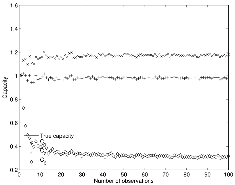
Figure 1: Comparison of various classical capacity estimators for various number of observations, model (4). $\sigma^{2}=0.1$, $n=10$ receive antennas, $m=10$ transmit antennas. The rank of ${\bf H}$ was $3$.

In figure 2, the same $\sigma$ and channel matrix are put to the test with the free-probability based and Gaussian matrix mean based estimators for various number of observations. These give values close to the true capacity. Both work better than $C_{3}$ for small number of observations.

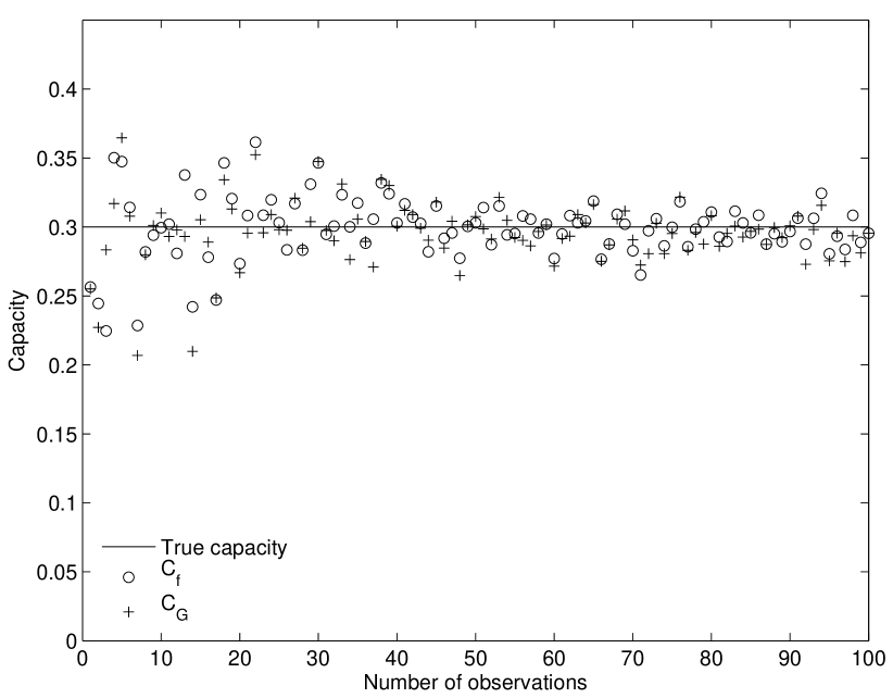
Figure 2: Comparison of $C_{f}$ and $C_{G}$ for various number of observations, model (4). $\sigma^{2}=0.1$, $n=10$ receive antennas, $m=10$ transmit antennas. The rank of ${\bf H}$ was $3$.

The free-probability based estimator converges faster (in terms of the number of observations) for lower rank channel matrices. In figure 3 we illustrate this for $10\times 10$ channel matrices of rank 3, 5 and 6.

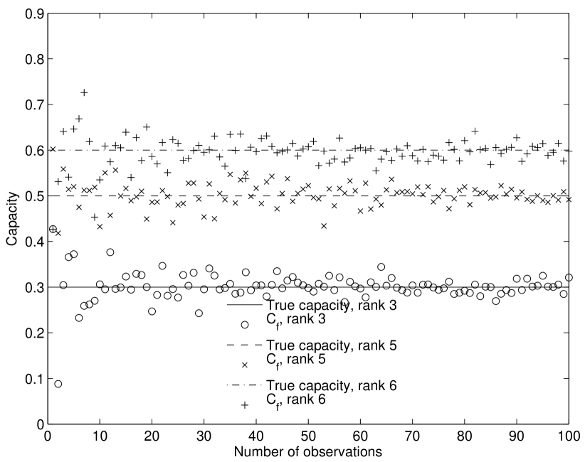
Figure 3: $C_{f}$ for various number of observations, model (4). $\sigma^{2}=0.1$, $n=10$ receive antennas, $m=10$ transmit antennas. The rank of ${\bf H}$ was $3$, $5$ and $6$.

Simulations show that for channel matrices of lower dimension (for instance $6\times 6$), we have slower convergence to the true capacity.

V-B Channels with phase off-set and phase drift

In figure 4, the $C_{3}$ estimator is compared with the free-probability based estimator, the Gaussian matrix mean based estimator and the true capacity, for various number of observations, and with the same $\sigma$ and channel matrix as in figure 1 and 2. Phase off-set and phase drift have also been introduced.

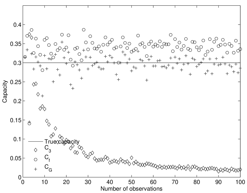
Figure 4: Comparison of capacity estimators which worked for model (4) for increasing number of observations. Model (3) is used. $\sigma^{2}=0.1$, $n=10$ receive antennas, $m=10$ transmit antennas. The rank of ${\bf H}$ was $3$.

In this case, the free-probability based estimator and the $C_{3}$-estimator seem to be biased.

In figure 5, simulations have been performed for various $\sigma$. Only $L=1$ observation was used, $n=10$ receive antennas, and $m=10$ transmit antennas. The channel matrix has rank $3$. It is seen that the Gaussian matrix mean based capacity estimator is very close to the true capacity, There are only small deviations even if one observation is present, which provides a very good candidate for channel estimation in highly time-varying environments. The deviations are higher for higher $\sigma$.

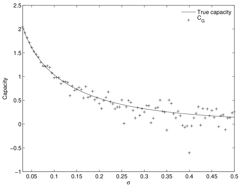
Figure 5: $C_{G}$ for $L=1$ observation, $n=10$ receive antennas, $m=10$ transmit antennas, with varying values of $\sigma$. Model (3). The rank of ${\bf H}$ was $3$.

In figure 6 we have also varied $\sigma$ and used only one observation, but we have formed another rank $3$ matrix with, $n=4$ receive antennas, $m=4$ transmit antennas. It is seen that the deviation from the true capacity is much higher in this case.

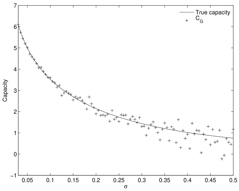
Figure 6: $C_{G}$ for $L=1$ observation, $n=4$ receive antennas, $m=4$ transmit antennas, with varying values of $\sigma$. Model (3). The rank of ${\bf H}$ was $3$.

We have in figure 7 increased the number of observations to $10$, and used the same channel matrix. It is seen that this decreases the deviation from the true capacity.

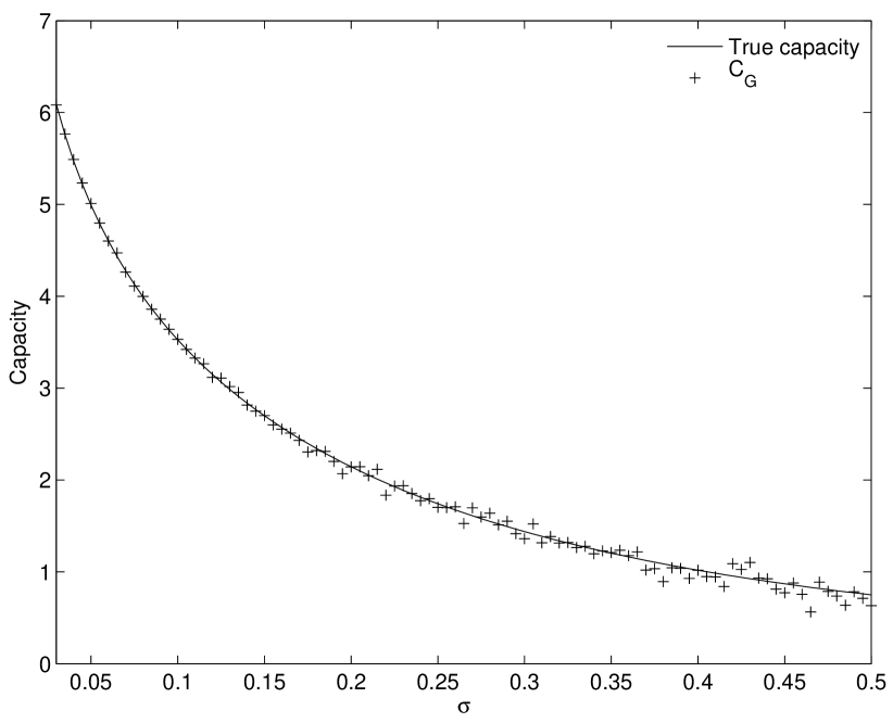
Figure 7: $C_{G}$ for $L=10$ observations, $n=4$ receive antennas, $m=4$ transmit antennas, with varying values of $\sigma$. Model (3). The rank of ${\bf H}$ was $3$.

Finally, let us use a channel matrix of rank $4$. In this case we have to increase the number of observations even further to accurately predict the channel capacity. In figure 8, Gaussian matrix mean based capacity estimation is performed for a rank $4$ channel matrix with $n=4$ receive antennas, $m=4$ transmit antennas. $1$ observation is performed. If we increase the number of observations, Gaussian matrix mean based capacity estimation is seen to go very slowly towards the true capacity. To illustrate this, figure 9 shows Gaussian matrix mean based capacity estimation for $10$ observations on the same channel matrix.

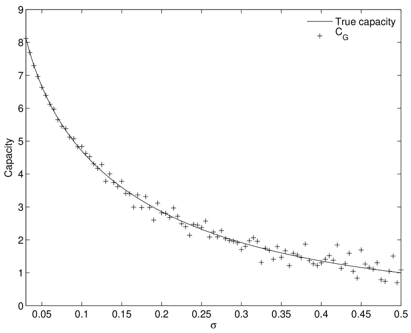
Figure 8: $C_{G}$ for $L=1$ observation, $n=4$ receive antennas, $m=4$ transmit antennas, with varying values of $\sigma$. Model (3). The rank of ${\bf H}$ was $4$.

It is seen that this decreases the deviation from the true capacity.

Figure 9: $C_{G}$ for $L=10$ observations, $n=4$ receive antennas, $m=4$ transmit antennas, with varying values of $\sigma$. Model (3). The rank of ${\bf H}$ was $4$.

VI Conclusion

In this paper, we have shown that free probability provides a neat framework for estimating the channel capacity for certain MIMO systems. In the case of highly time varying environments, where one can rely only on a set of limited noisy measurements, we have provided an asymptotically unbiased estimator of the channel capacity. A modified estimator called the Gaussian matrix mean based estimator was also introduced to take into account the bias in the case of finite dimensions and was proved to be adequate for low rank channel matrices. Moreover, although the results are based on asymptotic claims (in the number of observations), simulations show that the estimators work well for a very low number of observations also. Even when considering discrepancies such as phase drifts and phase off-set, the algorithm, based on the Gaussian matrix mean based estimator, provided very good performance. Further research is being conducted to take into account spatial correlation of the noise (in other words, deconvolving with other measures than the Marc̆henko Pastur law).

Appendix A The proof of proposition 2

Let $(m_{1},m_{2},...)$ be the moments of $\eta$, $(M_{1},M_{2},...)$ the moments of $\eta\boxtimes\mu_{c}$. Then [6]

$$\begin{array}[]{lll}cM_{1}&=&cm_{1}\\ cM_{2}&=&cm_{2}+c^{2}m_{1}^{2}\\ cM_{3}&=&cm_{3}+3c^{2}m_{1}m_{2}+c^{3}m_{1}^{3}\\ cM_{4}&=&cm_{4}+4c^{2}m_{1}m_{3}+2c^{2}m_{2}^{2}+6c^{3}m_{1}^{2}m_{2}+c^{4}m_{1}^{4}.\end{array}$$ (22)

Note that (22) can also be inverted to express the $m_{j}$ in terms of the $M_{j}$ instead:

$$\begin{array}[]{l}cm_{1}=cM_{1}\\ cm_{2}=cM_{2}-c^{2}M_{1}^{2}\\ cm_{3}=cM_{3}-3c^{2}M_{1}M_{2}+2c^{3}M_{1}^{3}\\ cm_{4}=cM_{4}-4c^{2}M_{1}M_{3}-2c^{2}M_{2}^{2}+10c^{3}M_{1}^{2}M_{2}-5c^{4}M_{1}^{4}.\end{array}$$ (23)

Note also that the moments of $\eta\boxplus\delta_{\sigma^{2}}$ are

$$\begin{array}[]{ll}&m_{1}+{\sigma}^{2}\\ &m_{2}+2{\sigma}^{2}m_{1}+{\sigma}^{4}\\ &m_{3}+3{\sigma}^{2}m_{2}+3{\sigma}^{4}m_{1}+{\sigma}^{6}\\ &m_{4}+4\sigma^{2}m_{3}+6{\sigma}^{4}m_{2}+4{\sigma}^{6}m_{1}+{\sigma}^{8}\end{array}$$ (24)

By the definition of the free probability based estimator,

$$\nu_{\frac{1}{m}\hat{\bf H}_{1...L}\hat{\bf H}_{1...L}^{H}}=\left(\left(\eta\begin{picture}(9.0,5.0)\put(2.0,0.0){\framebox(5.0,5.0)[]{$\smallsetminus$}} \end{picture}\mu_{\frac{1}{L}}\right)\boxplus\delta_{\sigma^{2}}\right)\boxtimes\mu_{\frac{1}{L}}$$

where the moments of $\eta$ are $h_{1},h_{2},h_{3},...$. Denoting by $\eta_{1}=\eta\begin{picture}(9.0,5.0)\put(2.0,0.0){\framebox(5.0,5.0)[]{$\smallsetminus$}} \end{picture}\mu_{\frac{1}{L}}$, $\eta_{2}=\eta_{1}\boxplus\delta_{\sigma^{2}}$, we have that $\nu_{\frac{1}{m}\hat{\bf H}_{1...L}\hat{\bf H}_{1...L}^{H}}=\eta_{2}\boxtimes\mu_{\frac{1}{L}}$. Denote also the moments of $\eta_{1}$ by $r_{i}$, the moments of $\eta_{2}$ by $s_{i}$, and as before the moments of $\frac{1}{m}\hat{\bf H}_{1...L}\hat{\bf H}_{1...L}^{H}$ by $\hat{h}_{1},\hat{h}_{2},\hat{h}_{3},...$. Write also $c=\frac{n}{mL}$ as in proposition 2. For the third moment, we can apply (22), (24) and (23) in that order,

$$\begin{array}[]{lll}\hat{h}_{3}&=&s_{3}+3cs_{1}s_{2}+c^{2}s_{1}^{3}\\ &=&r_{3}+3{\sigma}^{2}r_{2}+3{\sigma}^{4}r_{1}+{\sigma}^{6}\\ &&+3c(r_{1}+{\sigma}^{2})(r_{2}+2{\sigma}^{2}r_{1}+{\sigma}^{4})\\ &&+c^{2}(r_{1}+{\sigma}^{2})^{3}\\ &=&r_{3}+3cr_{1}r_{2}+c^{2}r_{1}^{3}\\ &&+3{\sigma}^{2}(1+c)r_{2}+(6c+3c^{2}){\sigma}^{2}r_{1}^{2}\\ &&+{\sigma}^{4}(3+9c+3c^{2})r_{1}+{\sigma}^{6}(1+3c+c^{2})\\ &=&h_{3}-3ch_{1}h_{2}+2c^{2}h_{1}^{3}\\ &&+3ch_{1}(h_{2}-ch_{1}^{2})+c^{2}h_{1}^{3}\\ &&+(6c+3c^{2}){\sigma}^{2}h_{1}^{2}+3{\sigma}^{2}(1+c)(h_{2}-ch_{1}^{2})\\ &&+{\sigma}^{4}(3+9c+3c^{2})h_{1}+{\sigma}^{6}(1+3c+c^{2})\\ &=&h_{3}+3{\sigma}^{2}(1+c)h_{2}+3{\sigma}^{2}ch_{1}^{2}\\ &&+3{\sigma}^{4}\left(c^{2}+3c+1\right)h_{1}+{\sigma}^{6}\left(c^{2}+3c+1\right),\end{array}$$

which is the third equation in (17) of proposition 2. Calculations are similar for the other moments, but more tedious for the fourth moment.

Appendix B The proof of proposition 1

In all the following, the matrices are of dimension $n\times N$. We need some terminology and results from [22] for the proof of proposition 1. Let $S_{p}$ be the set of permutations of $p$ elements $\{1,2,...,p\}$. For $\pi\in S_{p}$, let also $\hat{\pi}$ be the permutation in $S_{2p}$ defined by

$$\begin{array}[]{rcll}\hat{\pi}(2j-1)&=&2\pi^{-1}(j),&(j\in\{1,2,...,p\})\\ \hat{\pi}(2j)&=&2\pi(j)-1,&(j\in\{1,2,...,p\}),\end{array}$$ (25)

let ${\sim}_{\hat{\pi}}$ denote the equivalence relation on $\{1,...,2p\}$ generated by the expression

$$j{\sim}_{\hat{\pi}}\hat{\pi}(j)+1,\mbox{ (addition formed mod. $2p$)},$$ (26)

and let $k(\hat{\pi})$ and $l(\hat{\pi})$ denote the number of equivalence classes of ${\sim}_{\hat{\pi}}$ consisting of even numbers or odd numbers, respectively. Corollary 1.12 in [22] (slightly rewritten) states that

$$E\left[tr_{n}\left(\left(\frac{1}{N}{\bf X}{\bf X}^{H}\right)^{p}\right)\right]=\frac{1}{nN^{p}}\sum_{\pi\in S_{p}}N^{k(\hat{\pi})}n^{l(\hat{\pi})},$$ (27)

(9) can thus be proved by calculating all values of $k(\hat{\pi})$ and $l(\hat{\pi})$ for $\pi$ in $S_{1}$, $S_{2}$, $S_{3}$ and $S_{4}$. We prove here the case $p=3$, to get an idea on how the calculations are performed. For the six permutations in $S_{3}$ we obtain the following numbers by using (25) and (26):

$$\begin{array}[]{|l|l|l|l|}\hline\cr\pi&\mbox{Equivalence classes of }{\sim}_{\hat{\pi}}&k(\hat{\pi})&l(\hat{\pi})\\ \hline\cr(1,2,3)&\{\{1,3,5\},\{2\},\{4\},\{6\}\}&3&1\\ \hline\cr(1,3,2)&\{\{1,3\},\{2\},\{4,6\},\{5\}\}&2&2\\ \hline\cr(2,1,3)&\{\{1,5\},\{2,4\},\{3\},\{6\}\}&2&2\\ \hline\cr(2,3,1)&\{\{1\},\{2,4,6\},\{3\},\{5\}\}&1&3\\ \hline\cr(3,1,2)&\{\{1,3,5\},\{2,4,6\}\}&1&1\\ \hline\cr(3,2,1)&\{\{1\},\{2,6\},\{3,5\},\{4\}\}&2&2\\ \hline\cr\end{array}$$

Here $\pi=(i,j,k)$ means that $\pi(1)=i,\pi(2)=j,\pi(3)=k$. Putting the numbers into (27) we get

$$\begin{array}[]{l}E\left[tr_{n}\left(\left(\frac{1}{N}{\bf X}{\bf X}^{H}\right)^{p}\right)\right]\\ =\frac{1}{nN^{3}}\left(N^{3}n+N^{2}n^{2}+N^{2}n^{2}+Nn^{3}+Nn+N^{2}n^{2}\right)\\ =1+3\frac{n}{N}+\frac{n^{2}}{N^{2}}+\frac{1}{N^{2}}=1+3c+c^{2}+\frac{1}{N^{2}},\end{array}$$

which is the third equation in (9). We skip the computations for the other equations in (9), since they are very similar and quite tedious, since $S_{p}$ has $p!$ elements.

Appendix C The proof of theorems 2 and 3

We will first show the following:

Lemma 1

For systems of type (1), the following holds when ${\bf R}_{n}$ is deterministic:

$$\begin{array}[]{lll}E\left[tr_{n}\left({\bf W}_{n}\right)\right]&=&m_{1}+\sigma^{2}\\ E\left[tr_{n}\left({\bf W}_{n}^{2}\right)\right]&=&m_{2}+2{\sigma}^{2}(1+c)m_{1}+{\sigma}^{4}(1+c)\\ E\left[tr_{n}\left({\bf W}_{n}^{3}\right)\right]&=&m_{3}+3{\sigma}^{2}(1+c)m_{2}+3{\sigma}^{2}cm_{1}^{2}\\ &&+3{\sigma}^{4}\left(c^{2}+3c+1+\frac{1}{N^{2}}\right)m_{1}\\ &&+{\sigma}^{6}\left(c^{2}+3c+1+\frac{1}{N^{2}}\right)\\ E\left[tr_{n}\left({\bf W}_{n}^{4}\right)\right]&=&m_{4}+4{\sigma}^{2}(1+c)m_{3}+8{\sigma}^{2}cm_{2}m_{1}\\ &&+{\sigma}^{4}(6c^{2}+16c+6+\frac{16}{N^{2}})m_{2}\\ &&+14{\sigma}^{4}c(1+c)m_{1}^{2}\\ &&+4{\sigma}^{6}(c^{3}+6c^{2}+6c+1+\frac{5(c+1)}{N^{2}})m_{1}\\ &&+{\sigma}^{8}\left(c^{3}+6c^{2}+6c+1+\frac{5(c+1)}{N^{2}}\right),\end{array}$$ (28)

where $m_{j}=tr_{n}\left(\left(\frac{1}{N}{\bf R}_{n}{\bf R}_{n}^{H}\right)^{j}\right)$.

We remark that it is the assumption that ${\bf X}_{n}$ is Gaussian which makes the mixed moments $E\left[tr_{n}\left({\bf W}_{n}^{j}\right)\right]$ expressible in terms of the individual moments $m_{j}$. Without the Gaussian assumption, there is no reason why such a relationship should hold. Also, while our statements are made only for the four first moments, we remark that similar relationships can be written down for higher moments also, which deviate from corresponding free probability based estimates only in terms of the form $\frac{1}{N^{2k}}$ (that the deviation terms are on this form is actually a consequence of theorem 1.13 of [22]).

Before we prove lemma 1, let us explain how it proves theorems 2 and 3: We substitute $mL$ for $N$ (i.e. $c=\frac{n}{mL}$) for the case of $L$ observations, $m$ for $N$ (i.e. $c=\frac{n}{m}$) for the case of one observation, and ${\bf H}_{1...L}$ for ${\bf R}_{n}$ in lemma 1. Since the first two equations in (28) coincide with the corresponding first two formulas in (17) and (18), we see that the free probability based and the Gaussian matrix mean based estimators coincide for the first two moments in the case of only one observation, and that they are both unbiased for these two moments (regardless of which model is used). This proves the third statement of theorem 3, and the statements on $h_{f1}$ and $h_{f2}$ in theorem 2.

The third and fourth formulas in (18) are seen to equal the third and fourth formulas in (28), which explains why the Gaussian matrix mean based estimator has no bias in the third and fourth moments, thereby proving the first statement of theorem 3 (model (3) is also addressed due to the relationship (12)). The bias in the free probability based estimator is easily found by noting that the only differences between the third formula in (17) and the third formula in (28) are the terms $\frac{3{\sigma}^{4}}{m^{2}L^{2}}m_{1}$ and $\frac{{\sigma}^{6}}{m^{2}L^{2}}$. This proves statements 2 in theorem 2.

To see that $C_{G}$ is asymptotically unbiased when $m\rightarrow\infty$ (with $n,L$ kept fixed), it is sufficient to prove that the variance of all moments $tr_{n}({\bf W}_{n}^{k})$ go to zero. This will remedy the fact that the capacity is a non-linear expression of the moments. The proof for this part is a bit sketchy, since a similar analysis of such variances has already been done more throughly in connection with the theory of second order freeness [23]. We need to analyse

$$E\left(\left(tr_{n}({\bf W}_{n}^{k})\right)^{2}\right)-\left(E(tr_{n}({\bf W}_{n}^{k}))\right)^{2}.$$ (29)

This analysis is very similar to the one in the proof of lemma 1 below: One simply associates each term in ${\bf W}_{n}^{k}$ with a circle with $2k$ edges, and identify the edges which correspond to equal, Gaussian elements (this corresponds to the equivalence relation $\sim_{\hat{\pi}}$ of appendix B). Computation of $E\left(\left(tr_{n}({\bf W}_{n}^{k})\right)^{2}\right)$ and $\left(E(tr_{n}({\bf W}_{n}^{k}))\right)^{2}$ is thus reduced to counting the number of terms which give rise to the different identifications of the edges on two circles (one circle for each trace). We need only consider identifications which are pairings, due to the statements in appendix B when the matrix entries are Gaussian (see also [24, 22]).

One sees immediately that the edge identifications which can be found in $\left(E(tr_{n}({\bf W}_{n}^{k}))\right)^{2}$ is a subset of the edge identifications which can be found in $E\left(\left(tr_{n}({\bf W}_{n}^{k})\right)^{2}\right)$. These edge identifications therefore cancel each other in the expression for the variance, and we may therefore restrict to edge identifications which only appear in $E\left(\left(tr_{n}({\bf W}_{n}^{k})\right)^{2}\right)$. These correspond to the edge identifications where at least one identification across the two circles takes place. If we perform one such edge identification first, we are left with one circle with $4k-2$ edges (when the two identified edges are skipped). After the identification of the remaining edges, the vertices can be associated with a choice among the elements $\{1,...,N\}$, or a choice among the elements $\{1,...,n\}$ (matching with matrix dimensions). Similarly as in appendix B, let $k(\hat{\pi})$ denote the number of vertices of the first type, $l(\hat{\pi})$ the number of vertices of the second type. It is clear that $k(\hat{\pi})\leq 2k-1$ after the identification of edges. Since $N^{k(\hat{\pi})}\leq N^{2k-1}$ is not enough to cancel the leading $N^{2k}$-factor in $E\left(\left(tr_{n}({\bf W}_{n}^{k})\right)^{2}\right)$ (recall that only $N$ goes to infinity, not $n$), we conclude that (29) is $O\left(\frac{1}{N}\right)$, so that the variance of all moments go to $0$ as claimed, and we have established the second statement of theorem 3.

$C_{f}$ is, following the same reasoning, asymptotically unbiased when $L\rightarrow\infty$ or $m\rightarrow\infty$ for model (4), and when $L=1$ and $m\rightarrow\infty$ for model (3). This proves the two second statements in theorem 2, which concludes the proof of theorems 2 and 3.

Proof of lemma 1: Two facts are important in the proof. First of all, if $x_{1},...,x_{k}$ are standard i.i.d. complex Gaussian random variables, then, according to remark 2.2 in [24],

$$E(\left(x_{1}^{i_{1}}(\overline{x_{1}})^{j_{1}}\cdots x_{k}^{i_{k}}(\overline{x_{k}})^{j_{k}}\right)=0\mbox{ unless }i_{1}=j_{1},...,i_{k}=j_{k}.$$ (30)

Secondly, $E(|x_{i}|^{2p})=p!$ for such $x_{1},...,x_{k}$. we remark that the proof presented here can be simplified by using the following trick, taken from [22]: Rewrite a complex standard Gaussian random variable $x$ to the form $\frac{1}{\sqrt{s}}\left(x_{1}+\cdots+x_{s}\right)$, where $x_{1},...x_{s}$ are i.i.d. complex, standard, and Gaussian. ([22] uses this trick, and lets $s$ go to infinity).

Set ${\bf\Gamma}_{n}=\frac{1}{N}{\bf R}_{n}{\bf R}_{n}^{H}$. Let us first look at the case for the second moment. Note that

$$\begin{array}[]{lll}\lx@intercol\@ADDCLASS{ltx_eqn_lefteqn}$\displaystyle E\left[tr_{n}\left({\bf W}_{n}^{2}\right)\right]$\mbox{}\hfil\lx@intercol\\ &=&E\left[tr_{n}\left({\bf\Gamma}_{n}^{2}\right)\right]\\ &&+E\left[tr_{n}\left(\sigma^{2}\frac{1}{N^{2}}{\bf R}_{n}{\bf R}_{n}^{H}{\bf X}_{n}{\bf X}_{n}^{H}\right)\right]\\ &&+E\left[tr_{n}\left(\sigma^{2}\frac{1}{N^{2}}{\bf R}_{n}{\bf X}_{n}^{H}{\bf X}_{n}{\bf R}_{n}^{H}\right)\right]\\ &&+E\left[tr_{n}\left(\sigma^{2}\frac{1}{N^{2}}{\bf X}_{n}{\bf X}_{n}^{H}{\bf R}_{n}{\bf R}_{n}^{H}\right)\right]\\ &&+E\left[tr_{n}\left(\sigma^{2}\frac{1}{N^{2}}{\bf X}_{n}{\bf R}_{n}^{H}{\bf R}_{n}{\bf X}_{n}^{H}\right)\right]\\ &&+E\left[tr_{n}\left(\sigma^{4}\left(\frac{1}{N}{\bf X}_{n}{\bf X}_{n}^{H}\right)^{2}\right)\right]+E\left[tr_{n}\left(n_{2}\right)\right],\end{array}$$ (31)

where the terms in $n_{2}$ have expectation zero due to (30). We see that

• the first (deterministic) term is $m_{2}$, matching the first term in the second equation of (28),

• The next-to-last term is $\sigma^{4}(1+c)$, according to the second equation in (9). This matches the last term in the second equation of (28).

• By direct computation, the second term is

  $$\sigma^{2}\frac{1}{N^{2}n}\sum_{i,j,k,l}E\left({\bf R}_{n}(i,j){\bf R}_{n}^{H}(j,k){\bf X}_{n}(k,l){\bf X}_{n}^{H}(l,i).\right)$$

  This is nonzero only for $k=i$, so that this equals

  $$\begin{array}[]{l}\sigma^{2}\frac{1}{N^{2}n}\sum_{i,j}N{\bf R}_{n}(i,j){\bf R}_{n}^{H}(j,i)\\ =\sigma^{2}\frac{1}{N^{2}n}Nntr_{n}\left({\bf R}_{n}{\bf R}_{n}^{H}\right)\\ =\sigma^{2}tr_{n}\left(\frac{1}{N}{\bf R}_{n}{\bf R}_{n}^{H}\right)=\sigma^{2}m_{1}.\end{array}$$

• Similarly for the third term, which equals

  $$\begin{array}[]{l}\sigma^{2}\frac{1}{N^{2}n}\sum_{i,j,k,l}E\left({\bf R}_{n}(i,j){\bf X}_{n}^{H}(j,k){\bf X}(k,l){\bf R}_{n}^{H}(l,i)\right)\\ =\sigma^{2}\frac{1}{N^{2}n}nntr_{n}\left({\bf R}_{n}{\bf R}_{n}^{H}\right)=\sigma^{2}cm_{1}\end{array}$$

• The fourth and fifth term equal the second and third due to the trace property, so that the sum of the contributions of the second to fifth terms are $2\sigma^{2}(1+c)m_{1}$, which matches the second term in the second equation of (28).

Thus, contributions on the right hand side of (31) add up to the right hand side of the second equation in (28), proving the case for the second moment.

For the third moment, write

$$\begin{array}[]{l}E\left[tr_{n}\left({\bf W}_{n}^{3}\right)\right]=E\left[tr_{n}\left({\bf\Gamma}_{n}^{3}\right)\right]+\sigma^{2}E\left[tr_{n}\left((\alpha_{31}+\alpha_{32})\right)\right]\\ +\sigma^{4}E\left[tr_{n}\left((\beta_{31}+\beta_{32})\right)\right]+\sigma^{6}E\left[tr_{n}\left(\left(\frac{1}{N}{\bf X}_{n}{\bf X}_{n}^{H}\right)^{3}\right)\right]\\ +E\left[tr_{n}\left(n_{3}\right)\right]\end{array}$$ (32)

where the terms in $n_{3}$ all have expectation zero, and

$$\begin{array}[]{l}\alpha_{31}=\frac{1}{N^{3}}({\bf X}_{n}{\bf X}_{n}^{H}{\bf R}_{n}{\bf R}_{n}^{H}{\bf R}_{n}{\bf R}_{n}^{H}+{\bf R}_{n}{\bf X}_{n}^{H}{\bf X}_{n}{\bf R}_{n}^{H}{\bf R}_{n}{\bf R}_{n}^{H}\\ +{\bf R}_{n}{\bf R}_{n}^{H}{\bf X}_{n}{\bf X}_{n}^{H}{\bf R}_{n}{\bf R}_{n}^{H}+{\bf R}_{n}{\bf R}_{n}^{H}{\bf R}_{n}{\bf X}_{n}^{H}{\bf X}_{n}{\bf R}_{n}^{H}\\ +{\bf R}_{n}{\bf R}_{n}^{H}{\bf R}_{n}{\bf R}_{n}^{H}{\bf X}_{n}{\bf X}_{n}^{H}+{\bf X}_{n}{\bf R}_{n}^{H}{\bf R}_{n}{\bf R}_{n}^{H}{\bf R}_{n}{\bf X}_{n}^{H}),\end{array}$$

$$\begin{array}[]{l}\alpha_{32}=\frac{1}{N^{3}}({\bf X}_{n}{\bf R}_{n}^{H}{\bf R}_{n}{\bf X}_{n}^{H}{\bf R}_{n}{\bf R}_{n}^{H}+{\bf R}_{n}{\bf X}_{n}^{H}{\bf R}_{n}{\bf R}_{n}^{H}{\bf X}_{n}{\bf R}_{n}^{H}\\ +{\bf R}_{n}{\bf R}_{n}^{H}{\bf X}_{n}{\bf R}_{n}^{H}{\bf R}_{n}{\bf X}_{n}^{H}),\end{array}$$

$$\begin{array}[]{l}\beta_{31}=\frac{1}{N^{3}}({\bf R}_{n}{\bf R}_{n}^{H}{\bf X}_{n}{\bf X}_{n}^{H}{\bf X}_{n}{\bf X}_{n}^{H}+{\bf X}_{n}{\bf R}_{n}^{H}{\bf R}_{n}{\bf X}_{n}^{H}{\bf X}_{n}{\bf X}_{n}^{H}\\ +{\bf X}_{n}{\bf X}_{n}^{H}{\bf R}_{n}{\bf R}_{n}^{H}{\bf X}_{n}{\bf X}_{n}^{H}+{\bf X}_{n}{\bf X}_{n}^{H}{\bf X}_{n}{\bf R}_{n}^{H}{\bf R}_{n}{\bf X}_{n}^{H}\\ +{\bf X}_{n}{\bf X}_{n}^{H}{\bf X}_{n}{\bf X}_{n}^{H}{\bf R}_{n}{\bf R}_{n}^{H}+{\bf R}_{n}{\bf X}_{n}^{H}{\bf X}_{n}{\bf X}_{n}^{H}{\bf X}_{n}{\bf R}_{n}^{H}),\end{array}$$

$$\begin{array}[]{l}\beta_{32}=\frac{1}{N^{3}}({\bf R}_{n}{\bf X}_{n}^{H}{\bf X}_{n}{\bf R}_{n}^{H}{\bf X}_{n}{\bf X}_{n}^{H}+{\bf X}_{n}{\bf R}_{n}^{H}{\bf X}_{n}{\bf X}_{n}^{H}{\bf R}_{n}{\bf X}_{n}^{H}\\ +{\bf X}_{n}{\bf X}_{n}^{H}{\bf R}_{n}{\bf X}_{n}^{H}{\bf X}_{n}{\bf R}_{n}^{H})\end{array}$$

(i.e. the terms in $\alpha_{31},\beta_{31}$ have the terms ${\bf X}_{n}$,${\bf X}_{n}^{H}$ adjacent to each other). We see that

• the first and fourth terms in (32) match the first and fifth terms on the right hand side of the third equation in (28) (due to (9)).

• Three of the terms in $\alpha_{31}$ are seen to contribute with

  $$\frac{1}{N^{3}n}Nntr_{n}\left(\left({\bf R}_{n}{\bf R}_{n}^{H}\right)^{2}\right)=m_{2},$$

  and the remaining three terms are seen to contribute

  $$\frac{1}{N^{3}n}nntr_{n}\left(\left({\bf R}_{n}{\bf R}_{n}^{H}\right)^{2}\right)=cm_{2}$$

  Addition gives $\alpha_{31}=3(1+c)m_{2}$.

• All terms in $\alpha_{32}$ are seen to contribute

  $$\frac{1}{N^{3}n}nn\left(tr_{n}\left({\bf R}_{n}{\bf R}_{n}^{H}\right)\right)^{2}=cm_{1}^{2},$$

  so that the total contribution is $3cm_{1}^{2}$.

• Using the second formula in (9), three terms in $\beta_{31}$ are seen to contribute

  $$\frac{1}{Nn}ntr_{n}\left({\bf R}_{n}{\bf R}_{n}^{H}\right)\frac{1}{n}n(1+c)=(1+c)m_{1},$$

  and the remaining three terms contribute

  $$\frac{1}{Nn}ntr_{n}\left({\bf R}_{n}{\bf R}_{n}^{H}\right)\frac{1}{N}n(1+c)=c(1+c)m_{1},$$

  Addition gives $3(c^{2}+2c+1)m_{1}$.

• All terms in $\beta_{32}$ are seen to contribute

  $$\frac{1}{N^{3}n}ntr_{n}\left({\bf R}_{n}{\bf R}_{n}^{H}\right)(nN-1)+\frac{1}{N^{3}n}ntr_{n}\left({\bf R}_{n}{\bf R}_{n}^{H}\right)\times 2,$$

  where the factor $2$ comes in since $E(|x|^{4})=2$ for a complex standard Gaussian random variable. Simplifying we get $(c+\frac{1}{N^{2}})m_{1}$, so that the total contribution is $3(c+\frac{1}{N^{2}})m_{1}$

Thus, contributions on the right hand side of (32) add up to the right hand side of the third equation in (28), proving the case for the third moment also.

Now for the fourth equation in (28). The details in this are similar to the calculations for the third moment, but much more tedious. The first term for the fourth moment formula in (28) is trivial, as is the last term which comes from the fourth formula in (9). The second and third terms are calculated using exactly the same strategy as for the third moment. The remaining fourth, fifth and sixth terms require much attention. We address just some of these.

Computing $E\left[tr_{n}\left(\sigma^{6}(\beta_{41}+\beta_{42})\right)\right]$ gives the sixth term, where the terms in $\beta_{41}$ are similar to those for $\beta_{31}$ (i.e. the terms ${\bf X}_{n}$,${\bf X}_{n}^{H}$ are adjacent to each other), i.e. four terms have the same trace as

$$a=\frac{1}{N^{4}}{\bf R}_{n}{\bf R}_{n}^{H}{\bf X}_{n}{\bf X}_{n}^{H}{\bf X}_{n}{\bf X}_{n}^{H}{\bf X}_{n}{\bf X}_{n}^{H},$$

while four terms have the same trace as

$$b=\frac{1}{N^{4}}{\bf X}_{n}{\bf R}_{n}^{H}{\bf R}_{n}{\bf X}_{n}^{H}{\bf X}_{n}{\bf X}_{n}^{H}{\bf X}_{n}{\bf X}_{n}^{H},$$

It is clear that $E\left[tr_{n}(a)\right]$ equals

$$\frac{1}{N^{4}n}ntr_{n}\left({\bf R}_{n}{\bf R}_{n}^{H}\right)E\left[tr_{n}\left(\left({\bf X}_{n}{\bf X}_{n}^{H}\right)^{2}\right)\right]$$

$$= tr_{n}\left(\frac{1}{N}{\bf R}_{n}{\bf R}_{n}^{H}\right)E\left[tr_{n}\left(\left(\frac{1}{N}{\bf X}_{n}{\bf X}_{n}^{H}\right)^{2}\right)\right]$$

$$= \left(c^{2}+3c+1+\frac{1}{N^{2}}\right)m_{1},$$

and that $E\left[tr_{n}(b)\right]$ equals

$$\frac{1}{N^{4}n}ntr_{n}\left({\bf R}_{n}{\bf R}_{n}^{H}\right)cE\left[tr_{n}\left(\left({\bf X}_{n}{\bf X}_{n}^{H}\right)^{2}\right)\right]$$

$$= ctr_{n}\left(\frac{1}{N}{\bf R}_{n}{\bf R}_{n}^{H}\right)E\left[tr_{n}\left(\left(\frac{1}{N}{\bf X}_{n}{\bf X}_{n}^{H}\right)^{2}\right)\right]$$

$$= c\left(c^{2}+3c+1+\frac{1}{N^{2}}\right)m_{1},$$

so that $\beta_{41}=4(1+c)\left(c^{2}+3c+1+\frac{1}{N^{2}}\right)m_{1}$.

Similarly, for $\beta_{42}$ (where the terms ${\bf X}_{n}$,${\bf X}_{n}^{H}$ are not adjacent to each other), we need to address four terms which all have the same trace as

$$c=\frac{1}{N^{4}}{\bf R}_{n}{\bf X}_{n}^{H}{\bf X}_{n}{\bf R}_{n}^{H}{\bf X}_{n}{\bf X}_{n}^{H}{\bf X}_{n}{\bf X}_{n}^{H},$$

and four terms which have the same trace as

$$d=\frac{1}{N^{4}}{\bf X}_{n}{\bf R}_{n}^{H}{\bf X}_{n}{\bf X}_{n}^{H}{\bf R}_{n}{\bf X}_{n}^{H}{\bf X}_{n}{\bf X}_{n}^{H}.$$

By counting terms carefully, we see that these eight terms together contribute with $\left(8c+8c^{2}+\frac{16(c+1)}{N^{2}}\right)m_{1}$ (during this count of terms, we need the fact that $E(|x|^{6})=6$ when $x$ is complex, standard, and Gaussian). All in all we have that

$$E\left[tr_{n}\left(\sigma^{6}(\beta_{41}+\beta_{42})\right)\right]=$$

$$4\sigma^{6}(1+c)\left(c^{2}+3c+1+\frac{1}{N^{2}}\right)m_{1}+$$

$$\sigma^{6}\left(8c+8c^{2}+\frac{16(c+1)}{N^{2}}\right)m_{1}$$

$$= 4\sigma^{6}\left(c^{3}+6c^{2}+6c+1+\frac{5(1+c)}{N^{2}}\right)m_{1},$$

which is the sixth term in the fourth equation of (28).

The details for the fourth and fifth terms are dropped.             

As can be seen, the requirement that ${\bf R}_{n}$ is deterministic is not strictly necessary in the proof of lemma 1, so that we could replace it with any random matrix independent from ${\bf X}_{n}$, the moment $m_{j}$ with $E\left[tr_{n}\left(\left(\frac{1}{N}{\bf R}_{n}{\bf R}_{n}^{H}\right)^{j}\right)\right]$, and $m_{j}^{2}$ with $E\left[\left(tr_{n}\left(\left(\frac{1}{N}{\bf R}_{n}{\bf R}_{n}^{H}\right)^{j}\right)\right)^{2}\right]$.

References

- [1] E. Telatar, “Capacity of multi-antenna gaussian channels,” Eur. Trans. Telecomm. ETT, vol. 10, no. 6, pp. 585–596, Nov. 1999.
- [2] T. Guhr, A. Müller-Groeling, and H. A. Weidenmüller, “Random matrix theories in quantum physics: Common concepts,” Physica Rep., pp. 190–299, 1998.
- [3] J.-P. Bouchaud and M. Potters, Theory of Financial Risk and Derivative Pricing - From Statistical Physics to Risk Management. Cambridge: Cambridge University Press, 2000.
- [4] B. Dozier and J. W. Silverstein, “On the empirical distribution of eigenvalues of large dimensional information-plus-noise type matrices,” J. Multivariate Anal., vol. 98, no. 4, pp. 678–694, 2007.
- [5] Ø. Ryan and M. Debbah, “Multiplicative free convolution and information-plus-noise type matrices,” 2007, http://arxiv.org/abs/math.PR/0702342.
- [6] ——, “Free deconvolution for signal processing applications,” Submitted to IEEE Trans. on Information Theory, 2007, http://arxiv.org/abs/cs.IT/0701025.
- [7] R. L. de Lacerda Neto, L. Sampaio, R. Knopp, M. Debbah, and D. Gesbert, “EMOS platform: Real-time capacity estimation of MIMO channels in the UMTS-TDD band,” in International Symposium on Wireless Communication Systems, Trondheim, Norway, October 2007.
- [8] R. L. de Lacerda Neto, L. Sampaio, H. Hoffsteter, M. Debbah, D. Gesbert, and R. Knopp, “Capacity of MIMO systems: Impact of polarization, mobility and environment,” in IRAMUS Workshop, Val Thorens, France, January 2007.
- [9] J. P. Kermoal, L. Schumacher, K. I. Pedersen, P. E. Mogensen, and F. Frederiken, “A stochastic MIMO radio channel model with experimental validation,” IEEE Journal on Selected Areas in Communications, vol. 20, no. 6, pp. 1211–1225, 2002.
- [10] T. Pollet, M. V. Bladel, and M. Moeneclaey, “BER sensitivity of OFDM systems to carrier frequency offset and wiener phase noise,” IEEE Trans. on Communications, vol. 43, pp. 191–193, 1995.
- [11] P. H. Moose, “A technique for orthogonal frequency division multiplexing frequency offset correction,” IEEE Trans. on Communications, vol. 42, no. 10, pp. 2908–2914, 1994.
- [12] A. F. Molisch, M. Steinbauer, M. Toeltsch, E. Bonek, and R. Thoma, “Measurement of the capacity of MIMO systems in frequency-selective channels,” in IEEE 53rd Vehicular Technology Conference (VTC 2001 Spring), 2001, pp. 204 – 208.
- [13] E. Bonek, M. Steinbauer, H. Hofstetter, and C. F. Mecklenbräuker, “Double-directional radio channel measurements - what we can derive from them,” in URSI International Symposium on Signals, Systems, and Electronics (ISSSE’01), 2001, pp. 89 – 92.
- [14] H. Özcelik, M. Herdin, H. Hofstetter, and E. Bonek, “A comparison of measured 8x8 MIMO systems with a popular stochastic channel model at 5.2ghz,” in 10th International Conference on Telecommunications (ICT’2003), 2003, pp. 1542 – 1546.
- [15] E. Bonek, N. Czink, V. Holappa, M. Alatossava, L. Hentilä, J. Nuutinen, and A. Pal, “Indoor MIMO mearurements at 2.55 amd 5.25 ghz - a comparison of temporal and angular characteristics,” in Proceedings of the IST Mobile Summit 2006, 2006.
- [16] F. Hiai and D. Petz, The Semicircle Law, Free Random Variables and Entropy. American Mathematical Society, 2000.
- [17] A. M. Tulino and S. Verdú, Random Matrix Theory and Wireless Communications. www.nowpublishers.com, 2004.
- [18] A. Nica and R. Speicher, Lectures on the Combinatorics of Free Probability. Cambridge University Press, 2006.
- [19] R. Seroul and D. O’Shea, Programming for Mathematicians. Springer, 2000.
-
[20]
Ø. Ryan, Tools for estimating channel capacity, 2007,
http://ifi.uio.no/
~oyvindry/channelcapacity/. - [21] H. Bercovici and D. V. Voiculescu, “Free convolution of measures with unbounded support,” Indiana Univ. Math. J., vol. 42, no. 3, pp. 733–774, 1993.
- [22] U. Haagerup and S. Thorbjørnsen, “Random matrices and K-theory for exact -algebras.” [Online]. Available: citeseer.ist.psu.edu/114210.html
- [23] B. Collins, J. A. Mingo, P. Śniady, and R. Speicher, “Second order freeness and fluctuations of random matrices: III. higher order freeness and free cumulants,” Documenta Math., vol. 12, pp. 1–70, 2007.
- [24] S. Thorbjørnsen, “Mixed moments of Voiculescu’s Gaussian random matrices,” J. Funct. Anal., vol. 176, no. 2, pp. 213–246, 2000.