Robust hypothesis testing with a relative entropy tolerance

Abstract

This paper considers the design of a minimax test for two hypotheses where the actual probability densities of the observations are located in neighborhoods obtained by placing a bound on the relative entropy between actual and nominal densities. The minimax problem admits a saddle point which is characterized. The robust test applies a nonlinear transformation which flattens the nominal likelihood ratio in the vicinity of one. Results are illustrated by considering the transmission of binary data in the presence of additive noise.

I Introduction

Robust hypothesis testing and signal detection problems have been examined in detail over the last 40 years [2, 1]. The purpose of such studies is to design tests or detectors which are insensitive to modelling errors. Specifically, whereas standard Bayesian or Neyman-Pearson tests are designed for nominal observation probability distributions, their performance may degrade rapidly when the actual model deviates only moderately from the nominal model. To guard against modelling errors, a minimax framework is usually adopted for selecting tests or detectors. In this context, the goal is to design a test that minimizes the worst-case performance for all observation models in a properly specified neighborhood of the nominal model. For robust hypothesis testing, when the neighborhood of the nominal model under each hypothesis corresponds either to a contamination model or a proximity model based on the Kolmogorov metric or a variant thereof, Huber [3, 4, 2] showed that the minimax detector applies a clipping transformation to the nominal likelihood ratio function. The clipping effect is achieved by shifting small portions of the probability mass under each hypothesis to the tail sections where errors occur. This relatively minute shift of probability mass can result in a significant degradation in test performance.

We adopt here a minimax formulation of the robust hypothesis testing problem of the same type as [3, 4, 2]. The only difference is that the neighborhood where the actual observation probability density is located under each hypothesis is formed by placing an upper bound on the relative entropy of the actual density with respect to the nominal density. To justify the choice of the relative entropy as a measure of proximity between statistical models, observe that Huber’s work addresses primarily situations where statistical models are obtained directly from imperfect data, possibly contaminated by outliers. However there exists also situations where the densities employed in hypothesis testing are model based, arising from physical considerations, possibly with a few unknown parameters which are estimated from the data. In this context, the relative entropy is a natural metric for model mismatch, since it provides the underlying metric for establishing the convergence of the expectation-maximization method [5] of mathematical statistics. In fact from a differential geometric viewpoint, it is argued in [6] that the relative entropy forms a natural ‘distance’ between statistical models. More recently, in the context of estimation and filtering it was shown in [7, 8] that minimax filters based on a relative entropy tolerance take the form or risk-sensitive Wiener or Kalman filters, which have well known robustness properties. By selecting the relative entropy as a measure of model mismatch, a risk-sensitive viewpoint was also adopted recenty in [9] for developing robust macroeconomic policies. Given relative entropy neighborhoods of the nominal densities for the two hypotheses, it is easy to verify that a saddle point exists for the resulting minimax hypothesis testing problem. To identify the saddle point, two assumptions are made. First as in [3], it is assumed that the nominal likelihood ratio function (LR) is monotone increasing. Second, it is required that the nominal densities under the two hypotheses should be symmetric with respect to each other. This allows the parametrization of the robust test and least-favorable densities in terms of a single parameter which can be selected uniquely so that the relative entropy tolerance is satisfied. The least-favorable LR is expressed as a nonlinear transformation of the nominal LR. But, unlike [3, 4, 2], the transformation is not a clipping transformation. Instead, it attempts to drive the LR to a value as close one as possible. The least-favorable densities are divided into three segments. The extreme segments are scaled versions of the nominal densities, where the scaling aims at shifting some probability mass to tails where errors occur. But the middle segment is a section of the “mid-way density” on the geodesic linking the two nominal densities, where the mid-way density is characterized by the property that it has the same relative entropy with respect to each of the nominal densities.

The robust hypothesis testing problem we consider is also related to the worst-case noise detection problem examined in [10, 11], where given a binary communication system with additive noise, with the actual noise density located within a prespecified relative entropy bound of the nominal noise density, it is required to find the ML detector for the worst-case noise in the neighborhood of the nominal noise. Thus the difference between the problem we consider and [11] is that we allow the additive noise statistics to be different under each hypothesis, instead of forcing them to be the same. Finally, it is worth noting that [12] also examines robust hypothesis testing by using the relative entropy as a mismatch metric between actual and nominal densities, but it does so asymptotically as the number of measurements becomes infinite, so its results take a very different form.

The paper is organized as follows. Section II describes the minimax hypothesis problem with a relative entropy constraint. The saddle point of the problem is characterized in Section III, and examples are presented in Section IV. Finally, Section V gives some conclusions.

II Problem Formulation

Consider a binary hypothesis testing problem where under hypothesis $H_{j}$, with $j=0,\,1$, the random observation $Y\in\mathbb{R}$ admits $f_{j}(y)$ as nominal probability density. The actual density $g_{j}(y)$ of $Y$ under $H_{j}$ is not known exactly and belongs to the neighborhood

$${\cal F}_{j}=\{g_{j}:\,D(g_{j}|f_{j})\leq\epsilon_{j}\}\>,$$ (2.1)

where

$$D(g|f)=\int_{-\infty}^{\infty}\ln\big{(}\frac{g(y)}{f(y)}\big{)}g(y)dy$$ (2.2)

denotes the Kullback-Leibler (KL) divergence or relative entropy of probability densities $g(y)$ and $f(y)$. Note that the KL divergence is not a true distance since it is not symmetric, i.e., $D(g|f)\neq D(f|g)$, it does not satisfy the triangle inequality, but $D(g|f)\geq 0$ with equality if and only if $g=f$. Also, since $x\ln(x)$ is a convex function for $x\geq 0$, $D(g|f)$ is convex in $g$, which implies that neighborhood ${\cal F}_{j}$ is convex for $j=0,\,1$.

Let ${\cal D}$ denote the class of pointwise randomized decision rules $\delta(y)$ such that if $Y=y$, we select $H_{1}$ with probability $\delta(y)$ and $H_{0}$ with probability $1-\delta$, where $0\leq\delta(y)\leq 1$. Clearly ${\cal D}$ is convex, since if $\delta_{1}(y)$ and $\delta_{2}(y)$ are two decision rules of ${\cal D}$, then for $0\leq\alpha\leq 1$,

$$\delta(y)=\alpha\delta_{1}(y)+(1-\alpha)\delta_{2}(y)$$

also belongs to ${\cal D}$.

Let

$$P_{F}(\delta,g_{0}) = \int_{-\infty}^{\infty}\delta(y)g_{0}(y)dy$$ (2.3)

$$P_{M}(\delta,g_{1}) = \int_{-\infty}^{\infty}(1-\delta(y))g_{1}(y)dy$$ (2.4)

denote respectively the probability of false alarm and the probablity of a miss for decision rule $\delta\in{\cal D}$ when the densities of $Y$ under $H_{0}$ and $H_{1}$ are $g_{0}$ and $g_{1}$, respectively. Note that $P_{F}(\delta,g_{0})$ is separately linear in $\delta$ and $g_{0}$. Similarly $P_{M}(\delta,g_{1})$ is separately linear in $\delta$ and $g_{1}$. If we assume that the two hypotheses are equally likely, the probability of error of $\delta\in{\cal D}$ is given by

$$P_{E}(\delta,g_{0},g_{1})=\frac{1}{2}[P_{F}(\delta,g_{0})+P_{M}(\delta,g_{1})]\>.$$ (2.5)

We seek to solve the minimax problem

$$\min_{\delta\in{\cal D}}\max_{(g_{0},g_{1})\in{\cal F}_{0}\times{\cal F}_{1}}P_{E}(\delta,g_{0},g_{1})$$ (2.6)

Note that $P_{E}(\delta,g_{0},g_{1})$ is linear and thus convex in $\delta$. Similarly, it is linear and thus concave in $g_{0}$ and $g_{1}$. The set ${\cal F}_{0}\times{\cal F}_{1}$ is convex and compact, ${\cal D}$ is convex and since

$$||\delta||_{\infty}=\max_{y\in\mathbb{R}}\delta(y)$$

for all $\delta\in{\cal D}$, ${\cal D}$ is compact with respect to the infinity norm. So according to the Von Neumann minimax theorem [13, p. 319], there exists a saddle point $(\delta_{\mathrm{R}},(g_{0}^{\mathrm{L}},g_{1}^{\mathrm{L}}))$ for the minimax problem (2.6). Here $\delta_{\mathrm{R}}$ is the robust/minimax test, whereas $g_{0}^{\mathrm{L}}$ and $g_{1}^{\mathrm{L}}$ are the least favorable densities in ${\cal F}_{0}\times{\cal F}_{1}$. The saddle point is characterized by the property

$$P_{E}(\delta,g_{0}^{\mathrm{L}},g_{1}^{\mathrm{L}})\geq P_{E}(\delta_{\mathrm{R}},g_{0}^{\mathrm{L}},g_{1}^{\mathrm{L}})\geq P_{E}(\delta_{\mathrm{R}},g_{0},g_{1})$$ (2.7)

for all $\delta\in{\cal D}$, $g_{0}\in{\cal F}_{0}$ and $g_{1}\in{\cal F}_{1}$.

While it is nice to know that a saddle point exists, exhibiting a test $\delta_{\mathrm{R}}$ and least favorable densities $g_{j}^{\mathrm{L}}$, $j=0,\,1$ satisfying (2.7) is a nontrivial task. Before doing so, it is worth pointing out that the minimax problem (2.6) is of the same type as considered by Huber in [3, 4, 2]. The only difference is that the neighborhoods ${\cal F}_{j}$ differ from those considered in [2] which included contamination models or proximity models based on the Kolmogorov metric as special cases. The problem (2.6) is also closely related to the worst-case noise detection problem considered in [11], where for hypotheses

$$H_{0} : Y=-1+N$$

$$H_{1} : Y=1+N\>,$$ (2.8)

and a nominal probability density $f_{N}(n)$ for noise $N$, it was desired to construct a minimum probability of error detector for the least-favorable noise density $g_{N}(n)$ located in the KL ball specified by $D(g_{N}|f_{N})\leq\epsilon$. Thus the problem (2.6) differs from the one examined in [10, 11] by the fact that we allow the least-favorable noise distribution to be different under hypotheses $H_{0}$ and $H_{1}$, instead of insisting they should be the same.

III Saddle Point Specification

The first inequality of the saddle point characterization (2.7) indicates that the robust test $\delta_{\mathrm{R}}$ must be the optimum Bayesian test for the least-favorable pair $(g_{0}^{\mathrm{L}},g_{1}^{\mathrm{L}})$. So if

$$L_{\mathrm{L}}(y)=\frac{g_{1}^{\mathrm{L}}(y)}{g_{0}^{\mathrm{L}}(y)}$$ (3.1)

denotes the LR function for the pair $(g_{0}^{\mathrm{L}},g_{1}^{\mathrm{L}})$, we need to have

$$\delta_{\mathrm{R}}(y)=\left\{\begin{array}[]{ccl}1&\mbox{for}&L_{\mathrm{L}}(y)>1\\ \mbox{arbitrary}&\mbox{for}&L_{\mathrm{L}}(y)=1\\ 0&\mbox{for}&L_{\mathrm{L}}(y)<1\>.\end{array}\right.$$ (3.2)

Consider now the second inequality of (2.7). Because of the form (2.5) of $P_{E}(\delta,g_{0},g_{1})$, it is equivalent to

$$P_{F}(\delta_{\mathrm{R}},g_{0}^{\mathrm{L}}) \geq P_{F}(\delta_{\mathrm{R}},g_{0})$$

$$P_{M}(\delta_{\mathrm{R}},g_{1}^{\mathrm{L}}) \geq P_{M}(\delta_{\mathrm{R}},g_{1})$$

for all $g_{0}$ and $g_{1}$ in ${\cal F}_{0}$ and ${\cal F}_{1}$, respectively.

So, given $\delta_{\mathrm{R}}$, the least-favorable density $g_{0}^{\mathrm{L}}$ is obtained by maximizing $P_{F}(\delta_{\mathrm{R}},g_{0})$ for all functions $g_{0}\in{\cal F}_{0}$ such that

$$I(g_{0})=\int_{-\infty}^{\infty}g_{0}(y)dy=1\>.$$ (3.3)

Since $P_{F}(\delta_{\mathrm{R}},g_{0})$ is concave in $g_{0}$ and the domain ${\cal F}_{0}$ is convex, the maximization can be accomplished by using the method of Lagrange multipliers [14, Chap. 5]. Consider the Lagrangian

$$L(g_{0},\lambda,\mu)=P_{F}(\delta_{\mathrm{R}},g_{0})+\lambda(\epsilon_{0}-D(g_{0}|f_{0}))+\mu(1-I(g_{0}))$$ (3.4)

$$= \int_{-\infty}^{\infty}\big{[}\delta_{\mathrm{R}}(y)-\mu-\lambda\ln\big{(}\frac{g_{0}}{f_{0}}(y)\big{)}\big{]}g_{0}(y)dy+\lambda\epsilon_{0}+\mu\>,$$

where Lagrange multiplier $\lambda\geq 0$ is associated to the inequality constraint $D(g_{0}|f_{0})\leq\epsilon_{0}$, whereas multiplier $\mu$ corresponds to equality constraint (3.3). Note that the non-negativity constraint $g_{0}(y)\geq 0$ for the density function $g_{0}$ is not introduced explicitly, since the solution obtained below by maximizing $L$ satisfies this constraint automatically.

The Gateaux derivative [14, p. 17] of $L$ with respect to $g_{0}$ in the direction of an arbitrary function $z$ is given by

$$\nabla_{g_{0},z}L(g_{0},\lambda,\mu) = \lim_{h\rightarrow 0}\frac{1}{h}\big{[}L(g_{0}+hz,\lambda,\mu)-L(g_{0},\lambda,\mu)\big{]}$$ (3.5)

$$= \int_{-\infty}^{\infty}\big{[}\delta_{\mathrm{R}}-(\lambda+\mu)-\lambda\ln\big{(}\frac{g_{0}}{f_{0}}\big{)}\big{]}zdy\>,$$

and since $z(y)$ is arbitrary, this implies

$$\delta_{\mathrm{R}}(y)-(\lambda+\mu)-\lambda\ln\big{(}\frac{g_{0}}{f_{0}}\big{)}(y)=0\>.$$ (3.6)

In addition, the Karush-Kuhn-Tucker (KKT) condition

$$\lambda(\epsilon_{0}-D(g_{0}|f_{0}))=0$$ (3.7)

needs to be satisfied. Assume $\lambda>0$, so $D(g_{0}|f_{0})=\epsilon_{0}$, i.e., $g_{0}$ is on the boundary of ${\cal F}_{0}$. Then (3.6) implies

$$g_{0}^{\mathrm{L}}(y)=\frac{1}{Z_{0}}\exp(\alpha_{0}\delta_{\mathrm{R}}(y))f_{0}(y)$$ (3.8)

with

$$Z_{0}\stackrel{{\scriptstyle\triangle}}{{=}}\exp(1+\frac{\mu}{\lambda})\hskip 7.22743pt,\hskip 7.22743pt\alpha_{0}\stackrel{{\scriptstyle\triangle}}{{=}}\frac{1}{\lambda}\>.$$

Note that since the nominal density $f_{0}(y)\geq 0$ for all $y$, the least-favorable density $g_{0}^{\mathrm{L}}(y)$ specified by (3.8) is also non-negative, so that the non-negativity constraint on $g_{0}$ is satisfied automatically. Proceeding in a similar manner, we find that the least-favorable density under $H_{1}$ can be expressed as

$$g_{1}^{\mathrm{L}}(y)=\frac{1}{Z_{1}}\exp(\alpha_{1}(1-\delta_{\mathrm{R}}(y)))f_{1}(y)$$ (3.9)

with $Z_{1}>0$.

Together, the expressions (3.2) for $\delta_{\mathrm{R}}$ and (3.8)–(3.9) for $(g_{0}^{\mathrm{L}},g_{1}^{\mathrm{L}})$ provide some guidelines for guessing a saddle point satisfying inequalities (2.7). We exhibit below a saddle point with the desired structure under the following assumptions.

Assumptions:

• The nominal likelihood ratio

  $$L(y)=\frac{f_{1}(y)}{f_{0}(y)}$$ (3.10)

  is a monotone increasing function of $y$. This implies that $\ell=L(y)$ admits an inverse function $y=L^{-1}(\ell)$.

• $f_{0}(y)$ and $f_{1}(y)$ admit the symmetry

  $$f_{1}(y)=f_{0}(-y)\>.$$ (3.11)

  This assumption implies

  $$L(-y)=\frac{f_{1}(-y)}{f_{0}(-y)}=\frac{f_{0}(y)}{f_{1}(y)}=\frac{1}{L(y)}\>,$$

  and thus $L(0)=1$.

Remarks:

• The motonicity assumption for $L(y)$ appears also in [2]. The symmetry condition (3.11) has the effect of symmetrizing the KL divergence of $f_{0}$ and $f_{1}$, since it ensures

  $$D(f_{1}|f_{0})=D(f_{0}|f_{1})\>.$$

  Furthermore, for $0\leq u\leq 1$, if we consider the geodesic

  $$f_{u}(y)=\frac{f_{1}^{u}(y)f_{0}^{1-u}(y)}{Z(u)}$$

  linking nominal densities $f_{0}$ and $f_{1}$, where

  $$Z(u)=\int_{-\infty}^{\infty}f_{1}^{u}(y)f_{0}^{1-u}(y)dy\>,$$

  the assumption ii) ensures that the density $f_{1/2}$ is located mid-way between $f_{0}$ and $f_{1}$ in terms of the KL divergence, since

  $$D(f_{1/2}|f_{0})=D(f_{1/2}|f_{1})\>.$$

  We refer the reader to [15, Chap. 4.] and [6] for a detailed discussion of the differential geometric structure of statistical models.

• For model (2.8), the above assumptions are satisfied if under both hypotheses $N$ admits a generalized Gaussian density

  $$f_{N}(n)=a\exp(-|n/b|^{\alpha})$$

  with $\alpha>1$, where the constants $a$ and $b$ are adjusted to fix the variance of the distribution and normalize its total probability mass. The case $\alpha=2$ corresponds to a standard Gaussian distribution. On the other hand, if $N$ is Cauchy distributed, it is easy to verify that

  $$L(y)=\frac{f_{N}(y-1)}{f_{N}(y+1)}$$

  is not monotone increasing so Assumption i) is not satisfied.

• The assumptions allow the consideration of nonsymmetric noise distributions. For example, consider model (2.8) where under $H_{1}$, $N$ admits the asymmetric Laplace density

  $$f_{L}(n)=\left\{\begin{array}[]{cc}c\exp(-an)&n\geq 0\\ c\exp(bn)&n\leq 0\end{array}\right.$$ (3.12)

  with $b>a>0$ and $c=(a^{-1}+b^{-1})^{-1}$, and under $H_{0}$, $N$ admits the flipped density $f_{L}(-n)$. Then

  $$f_{1}(y)=f_{L}(y-1)\hskip 7.22743pt\mbox{and}\hskip 7.22743ptf_{0}(y)=f_{L}(-(y+1))$$

  satisfy the symmetry condition (3.11) and the log-likelihood ratio

  $$\ln L(y)=\ln(f_{1}(y)/f_{0}(y))=\left\{\begin{array}[]{cc}(b-a)y+(b+a)&y\geq 1\\ 2by&-1\leq y\leq 1\\ (b-a)y-(b+a)&y\leq-1\end{array}\right.$$ (3.13)

  is monotone increasing. Note that this property requires $b>a$, which ensures that the fat tails of $f_{1}(y)$ and $f_{0}(y)$ are located on the opposite side of the location parameter of the competing hypothesis. For example under $H_{1}$, the location parameter (the constant additive term in (2.8)) is $1$ so the fat tail extends over $[1,\infty)$, which is on the opposite side of the location parameter $-1$ of the competing hypothesis $H_{0}$.

We can now prove the following result.

Theorem 1

Assume that constants $\epsilon_{j}$ specifying neighborhoods ${\cal F}_{j}$ with $j=0,\,1$ are such that $\epsilon_{0}=\epsilon_{1}=\epsilon$, where

$$0<\epsilon<D(f_{1/2}|f_{0})\>.$$ (3.14)

This requirement ensures that ${\cal F}_{0}$ and ${\cal F}_{1}$ do not intersect. Then under assumptions i)-ii) consider the decision rule

$$\delta_{\mathrm{R}}(y)=\left\{\begin{array}[]{cc}1&y>y_{U}\\[4.30554pt] \displaystyle\frac{1}{2}\big{[}1+\frac{\ln L(y)}{\ln\ell_{U}}\big{]}&-y_{U}\leq y\leq y_{U}\\[4.30554pt] 0&y<-y_{U}\>,\end{array}\right.$$ (3.15)

and the least-favorable pair

$$g_{0}^{\mathrm{L}}(y) = \left\{\begin{array}[]{cc}\ell_{U}f_{0}(y)/Z(y_{U})&y>y_{U}\\ \ell_{U}^{1/2}f_{1}^{1/2}(y)f_{0}^{1/2}(y)/Z(y_{U})&-y_{U}\leq y\leq y_{U}\\ f_{0}(y)/Z(y_{U})&y<-y_{U}\end{array}\right.$$ (3.19)

$$g_{1}^{\mathrm{L}}(y) = \left\{\begin{array}[]{cc}f_{1}(y)/Z(y_{U})&y>y_{U}\\ \ell_{U}^{1/2}f_{1}^{1/2}(y)f_{0}^{1/2}(y)/Z(y_{U})&-y_{U}\leq y\leq y_{U}\\ \ell_{U}f_{1}(y)/Z(y_{U})&y<-y_{U}\end{array}\right.$$ (3.23)

which are parametrized by $y_{U}>0$ and $\ell_{U}=L(y_{U})>1$. Here the normalizing constant $Z(y_{U})$ is selected such that

$$I(g_{0}^{\mathrm{L}})=I(g_{1}^{\mathrm{L}})=1\>.$$ (3.24)

There exists a unique $y_{U}>0$ such that

$$D(g_{0}^{\mathrm{L}}|f_{0})=D(g_{1}^{\mathrm{L}}|f_{1})=\epsilon\>,$$ (3.25)

and the corresponding $\delta_{\mathrm{R}}$ and densities $(g_{0}^{\mathrm{L}},g_{1}^{\mathrm{L}})$ form a saddle point of minimax problem (2.6).

Before proving the result, it is worth noting that the least-favorable LR

$$L_{\mathrm{L}}(y)=\left\{\begin{array}[]{cc}\displaystyle\frac{L(y)}{\ell_{U}}>1&y>y_{U}\\[4.30554pt] 1&-y_{U}\leq y\leq y_{U}\\ \ell_{U}L(y)<1&y<-y_{U}\end{array}\right.$$ (3.26)

can be viewed as obtained by applying a nonlinearity $q(\cdot)$ to the nominal likelihood ratio $L$. Specifically, we have

$$L_{\mathrm{L}}=q(L)=\left\{\begin{array}[]{cc}L/\ell_{U}&L>\ell_{U}\\ 1&\ell_{U}^{-1}\leq L\leq\ell_{U}\\ \ell_{U}L&L<\ell_{U}^{-1}\end{array}\right.$$ (3.27)

where the nonlinearity $q(\cdot)$ is sketched in Fig. 1 below. This nonlinearity is different from the clipping transformation obtained by Huber [3, 4, 2] which truncates high and low values of the nominal likelihood ratio. Instead, the transformation $q(\cdot)$ attempts to force the transformed values $L_{\mathrm{L}}$ to be as close to $1$ as possible, where a LR value $L_{\mathrm{L}}=1$ corresponds to a situation where observation $Y=y$ is uninformative in terms of making a decision between $H_{1}$ and $H_{0}$.

in 0.01 l:0.08 w:0.05 t:F

(2.8 0) h:L v:C (0.1 0)$L$ (0.3 -0.3) (0 1.8) h:L v:C (0.1 0)$q(L)$ (0.3 0) (0.6 0.9) (0.75 0) (0.675 0.45) (0.05 0.05) (0.3 0.9) h:R v:C (-0.1 0)$1$ (0.6 0) (0 -0.9) h:C v:T (0 -0.1)$1/\ell_{U}$ (1.65 0) h:C v:T (0 -0.1)$\ell_{U}$ (0 0.9) (0.15 -0.15) h:C v:C (0 0)$0$ (1.85 1.25) h:C v:C (0 0)$L/\ell_{U}$ (0.65 0.25) h:C v:C (0 0)$\ell_{U}L$

Figure 1: Nonlinearity $q(\cdot)$ relating the nominal and least-favorable likelihood ratios.

Proof: Observe first that since the least-favorable LR is given by (3.26), the decision rule $\delta_{\mathrm{R}}$ specified by (3.15) has the form (3.2). Note that since $\ell_{U}^{-1}\leq L(y)\leq\ell_{U}$ for $-y_{U}\leq y\leq y_{U}$, we have

$$-1\leq\frac{\ln L(y)}{\ln\ell_{U}}\leq 1$$

for $-y_{U}\leq y\leq y_{U}$, which ensures $0\leq\delta_{\mathrm{R}}(y)\leq 1$ for $-y_{U}\leq y\leq y_{U}$.

Next, with $\delta_{\mathrm{R}}$ given by (3.15). it is easy to verify that the least favorable densities $g_{0}^{\mathrm{L}}$ and $g_{1}^{\mathrm{L}}$ given by (3.19) and (3.23) admit the forms (3.8) and (3.9) with $Z_{0}=Z_{1}=Z(y_{U})$ and

$$\alpha_{0}=\alpha_{1}=\ln\ell_{U}\>.$$

To ensure that the normalization condition (3.24) holds we only need to select

$$Z(y_{U})=\int_{-\infty}^{-y_{U}}f_{0}(y)dy+\ell_{U}^{1/2}\int_{-y_{U}}^{y_{U}}f_{1}^{1/2}(y)f_{0}^{1/2}(y)dy+\ell_{U}\int_{y_{U}}^{\infty}f_{0}(y)dy\>.$$

Then if $g_{0}^{\mathrm{L}}(\cdot|y_{U})$ represents the function (3.19), where the parametrization by $y_{U}\geq 0$ is written explicitly, let

$$D(y_{U}) \stackrel{{\scriptstyle\triangle}}{{=}} D(g_{0}^{\mathrm{L}}(\cdot|y_{U})|f_{0})$$ (3.28)

$$= -\ln Z(y_{U})+\frac{1}{Z(y_{U})}\Big{[}\ell_{U}\ln\ell_{U}\int_{y_{U}}^{\infty}f_{0}(y)dy$$

$$\hskip 72.26999pt+\ell_{U}^{1/2}\ln\ell_{U}\int_{0}^{y_{U}}f_{1}^{1/2}(y)f_{0}^{1/2}(y)dy\Big{]}$$

denote its KL divergence with respect to the nominal density $f_{0}$. For $y_{U}=0$, we have $g_{0}^{\mathrm{L}}(\cdot|0)=f_{0}$, so $D(0)=0$. Furthermore for $y_{U}=+\infty$, we have $g_{0}^{\mathrm{L}}(\cdot|+\infty)=f_{1/2}$, so $D(+\infty)=D(f_{1/2}|f_{0})$, where as noted earlier the density $f_{1/2}$ represents the mid-way point on the geodesic linking $f_{0}$ to $f_{1}$.

Taking the derivative of $D(y_{U})$ with respect to $y_{U}$ gives

$$\frac{dD}{dy_{U}} = -Z^{-1}(y_{U})\frac{dZ}{dy_{U}}$$ (3.29)

$$-Z^{-2}(y_{U})\frac{dZ}{dy_{U}}\Big{[}\ell_{U}\ln\ell_{U}\int_{y_{U}}^{\infty}f_{0}(y)dy+l_{U}^{1/2}\ln\ell_{U}\int_{-y_{U}}^{y_{U}}f_{1}^{1/2}(y)f_{0}^{1/2}(y)dy\Big{]}$$

$$+Z^{-1}(y_{U})\Big{[}\frac{d~{}}{dy_{U}}(\ell_{U}\ln\ell_{U})\int_{y_{U}}^{\infty}f_{0}(y)dy+\frac{d~{}}{dy_{U}}(\ell_{U}^{1/2}\ln\ell_{U})\int_{0}^{y_{U}}f_{1}^{1/2}(y)f_{0}^{1/2}(y)dy\Big{]}$$

$$= \frac{N(y_{U})}{Z^{2}(y_{U})}\frac{dL}{dy_{U}}\>,$$

where

$$N(y_{U})=\ln\ell_{U}\int_{y_{U}}^{\infty}f_{0}(y)dy\int_{y_{U}}^{\infty}f_{1}(y)dy$$

$$\hskip 14.45377pt+\frac{1}{2}\ln\ell_{U}\Big{[}\ell_{U}^{1/2}\int_{0}^{y_{U}}f_{1}^{1/2}(y)f_{0}^{1/2}(y)dy+\int_{y_{U}}^{\infty}\big{(}f_{0}(y)+\frac{f_{1}(y)}{\ell_{U}}\big{)}dy\Big{]}>0$$

for $y_{U}>0$. Since $L(y)$ is monotone increasing, we have $dL/dy_{U}>0$ in (3.29), so $dD/dy_{U}>0$. Consequently, $D(y_{U})$ is monotone increasing from $D(0)=0$ for $y_{U}=0$ to $D(f_{1/2}|f_{0})$ for $y_{U}=\infty$. Accordingly, given $\epsilon$ satisfying (3.14), there exists a unique $y_{U}$ such that $D(y_{U})=\epsilon$. For this choice of $y_{U}$, the least favorable densities $g_{0}^{\mathrm{L}}$ and $g_{1}^{\mathrm{L}}$ satisfy KKT condition (3.9), so the second inequality of (2.8) is satisfied, and $\delta_{\mathrm{R}}$ together with $(g_{0}^{\mathrm{L}},g_{1}^{\mathrm{L}})$ form the desired saddle point. $\Box$

Worst case test performance: By taking into account the symmetries

$$1-\delta_{\mathrm{R}}(y) = \delta_{\mathrm{R}}(-y)$$

$$g_{1}^{\mathrm{L}}(y) = g_{0}^{\mathrm{L}}(-y)$$ (3.30)

of the robust test and least favorable densities, which are a consequence of the symmetry assumption (3.11), we find that the worst-case probabilities of false alarm and of a miss for test $\delta_{\mathrm{R}}$ satisfy

$$P_{F}(\delta_{\mathrm{R}},g_{0}^{\mathrm{L}})=P_{M}(\delta_{\mathrm{R}},g_{1}^{\mathrm{L}})=P_{E}(\delta_{\mathrm{R}},g_{0}^{\mathrm{L}},g_{1}^{\mathrm{L}})\>,$$

where

$$P_{F}(\delta_{\mathrm{R}},g_{0}^{\mathrm{L}}) = \int_{-y_{U}}^{y_{U}}\delta_{\mathrm{R}}(y)g_{0}^{\mathrm{L}}(y)dy+Z^{-1}(y_{U})\ell_{U}\int_{y_{U}}^{\infty}f_{0}(y)dy$$ (3.31)

$$= Z^{-1}(y_{U})\Big{[}\ell_{U}^{1/2}\int_{0}^{y_{U}}f_{1}^{1/2}(y)f_{0}^{1/2}(y)dy+\ell_{U}\int_{y_{U}}^{\infty}f_{0}(y)dy\Big{]}\>.$$

IV Examples

Example 1: Consider the case where under $H_{0}$ and $H_{1}$, $Y$ admits the nominal distributions

$$f_{0}(y) = \frac{1}{(2\pi\sigma^{2})^{1/2}}\exp\big{(}-\frac{(y+1)^{2}}{2\sigma^{2}}\big{)}$$

$$f_{1}(y) = \frac{1}{(2\pi\sigma^{2})^{1/2}}\exp\big{(}-\frac{(y-1)^{2}}{2\sigma^{2}}\big{)}\>.$$ (4.1)

This corresponds to a model of the form (2.8) where the additive noise $N$ has a $N(0,\sigma^{2})$ nominal distribution. The signal to noise ratio (SNR) for this detection problem is $\mathrm{SNR}=1/\sigma^{2}$. The likelihood ratio

$$L(y)=\frac{f_{1}(y)}{f_{0}(y)}=\exp\big{(}\frac{2y}{\sigma^{2}}\big{)}$$

is clearly monotone increasing, and the nominal densities $f_{j}(y)$, $j=0,\,1$ admit the symmetry (3.11), so the assumptions of Theorem 1 are satisfied. In this case, it is interesting to note that the mid-way density

$$f_{1/2}(y)=\frac{f_{1}^{1/2}(y)f_{0}^{1/2}(y)}{Z(1/2)}=\frac{1}{(2\pi\sigma^{2})^{1/2}}\exp\big{(}-\frac{y^{2}}{2\sigma^{2}}\big{)}\>,$$

is $N(0,\sigma^{2})$ distributed, which makes sense since $f_{0}$ and $f_{1}$ have opposite means $\mp 1$ but the same variance $\sigma^{2}$.

If we consider the parametrization (3.19) of the least favorable density $g_{0}^{\mathrm{L}}(y)$, we find that it is continuous and formed by three segments. Over $(-\infty,-y_{U})$, $g_{0}^{\mathrm{L}}$ is an attenuated version of the nominal $N(-1,\sigma^{2})$ density. Over $[-y_{U},y_{U}]$, it is a scaled version of the mid-way $N(0,\sigma^{2})$ density, and for $(y_{U},\infty)$ it is an amplified version of the nominal $N(-1,\sigma^{2})$ density. Thus $g_{0}^{\mathrm{L}}$ can be viewed as obtained from the nominal density $f_{0}$ by shifting a portion of its probability mass to the middle segment where $g_{0}^{\mathrm{L}}$ and $g_{1}^{\mathrm{L}}$ are equal, and to the right tail where hypothesis $H_{1}$ is selected, which has the effect of increasing the probability of false alarm.

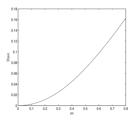
Figure 2: Plot of function $D(y_{U})$ for $0$dB SNR.

To illustrate the construction of $g_{0}^{\mathrm{L}}(y)$, let the relative entropy tolerance be $\epsilon=0.1$. Then for a nominal SNR equal to $0$dB ($\sigma=1$), the function $D(y_{U})$ measuring the KL divergence of $g_{0}^{\mathrm{L}}(\cdot|y_{U})$ with respect to $f_{0}$ is plotted in Fig. 2. As expected, it is monotone increasing and attains the desired tolerance value $\epsilon=0.1$ for $y_{U}=0.6080$. The least-favorable density $g_{0}^{\mathrm{L}}(y)$ is plotted together with the nominal density $f_{0}(y)$ in part a) of Fig. 3.

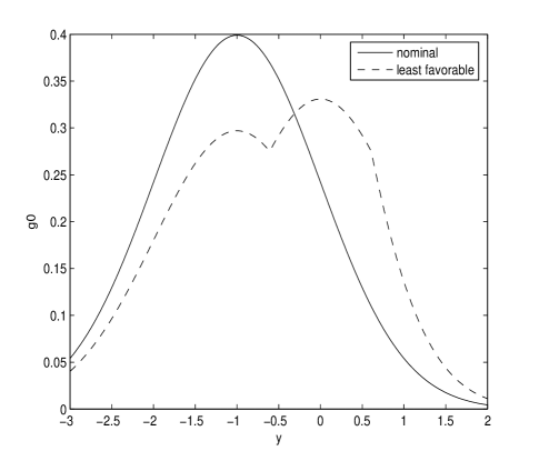
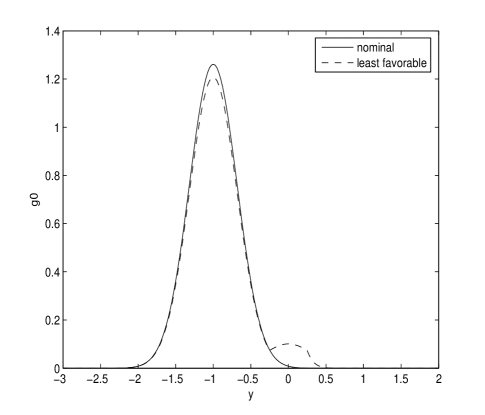
(a) (b)

Figure 3: Least favorable density $g_{0}^{\mathrm{L}}(y)$ for a tolerance $\epsilon=0.1$ and a) SNR =0dB, b) SNR = 10dB.

The three segments of the density described earlier are clearly in evidence in this plot. Note however that as the SNR increases, the middle segment shrinks. For example, the least-favorable density for a SNR value of $10$dB is shown in part b) of Fig. 3. Although the KL tolerance $\epsilon=0.1$ is the same as in part a), the deviation of $g_{0}^{\mathrm{L}}$ away from $f_{0}$ is much smaller than for a SNR value of 0dB. Note also that $g_{0}^{\mathrm{L}}$ is not symmetric about $-1$ since a fraction of the probability mass has been transferred from the left tail to the right tail in the direction of the location parameter $1$ of the competing hypothesis $H_{1}$. Similarly the least favorable distribution $g_{1}^{\mathrm{L}}(y)=g_{0}^{\mathrm{L}}(-y)$ transfers a portion of its probability mass from its right tail to its left tail. In terms of model (2.8), this means that the least favorable densities of the noise $N$ are different under $H_{0}$ and $H_{1}$, since one tilts rightward while the other tilts leftward. In contrast, [11] requires that the least-favorable noise should be the same under both hypotheses. For the above example with $\epsilon=0.1$ and $10$dB SNR, the least favorable noise density is plotted in the SouthWest corner of Figure 3 of [11]. It is symmetric and thus differs from the least-favorable densities obtained here.

Finally, for $\epsilon=0.01$ and $0.1$, and for SNR values between $0$ and $15$dB, the worst-case performance of the robust test $\delta_{\mathrm{R}}$ given by (3.31) is compared in Fig. 4 with the probability of error $P_{E}=Q(\mathrm{SNR}^{1/2})$ of the maximum likelihood detector for nominal densities (4.1). As indicated by the figure, the loss of performance is rather spectacular. Of course, since this performance represents a worst case situation, it is not truly indicative of the degradation incurred for more benign choices of densities $g_{j}$ in ${\cal F}_{j}$ with $j=0,\,1$.

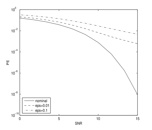
Figure 4: Comparison of the worst case probability of error of test $\delta_{\mathrm{R}}$ for $\epsilon=0.01$ and $\epsilon=0.1$ with the ML probability of error for the nominal model.

Example 2: Consider model (2.8) where under $H_{1}$ $N$ admits the asymmetric Laplace density $f_{L}(n)$ given by (3.12) with $b>a$ and under $H_{0}$, $N$ admits the flipped density $f_{L}(-n)$. Then the densities

$$f_{1}(y)=f_{L}(y-1)\hskip 7.22743pt,\hskip 7.22743ptf_{0}(y)=f_{L}(-(y+1))$$

satisfy the symmetry condition (3.11), and as indicated by (3.13), the likelihood ratio $L(y)$ is monotone increasing. In this case, the half-way density

$$f_{1/2}(y) = \frac{f_{0}^{1/2}(y)f_{1}^{1/2}(y)}{Z(1/2)}$$ (4.4)

$$= \left\{\begin{array}[]{cc}c\exp(-b)/Z(1/2)&-1\leq y\leq 1\\[4.30554pt] c\exp\big{(}-\frac{a+b}{2}|y|+\frac{a-b}{2}\big{)}/Z(1/2)&|y|\geq 1\end{array}\right.$$

with

$$Z(1/2)=2c\exp(-b)\big{(}1+\frac{2}{a+b}\big{)}$$

is constant for $-1\leq y\leq 1$ and has a symmetrized exponential decay rate for its two tails. For $y_{U}<1$, the parametrization (3.19) of the least favorable density $g_{0}^{\mathrm{L}}$ indicates that over segments $(-\infty,-y_{U})$ and $(y_{U},\infty)$ it is proportional to $f_{0}$, but over $[-y_{U},y_{U}]$ it is constant since $f_{1/2}$ is constant.

To illustrate this feature the nominal and least favorable densities are plotted in Fig. 5 for $a=2$, $b=4$, and $\epsilon=0.1$. For this choice of parameters $y_{U}=0.3640$.

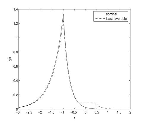
Figure 5: Nominal asymmetric Laplace density $f_{0}$ and least favorable density $g_{0}^{\mathrm{L}}$ for $a=2$, $b=4$ and tolerance $\epsilon=0.1$.

V Conclusion

A minimax hypothesis testing procedure has been derived for a binary hypothesis testing problem where the actual observation density under each hypothesis is required to be within a fixed KL ball centered about the nominal density. The robust test applies a nonlinear transformation which flattens the nominal LR in the vicinity of $L=1$. The least-favorable densities include three segments where, quite interestingly, the middle segment is formed by a section of the density located mid-way on the geodesic linking the nominal densities under the two hypotheses.

The results were derived under a motonicity condition for the LR as well as a symmetry condition for the two hypotheses. While the first condition is benign and appears in Huber’s work [3, 4, 2], it would be desirable to remove the symmetry condition (3.11), since this would open the way to the study of more general robust signal detection problems of the type discussed in [1].

References

- [1] S. A. Kassam and H. V. Poor, ”Robust techniques for signal processing: a survey”, Proc. IEEE, vol. 73, pp. 433–482, March 1985.
- [2] P. J. Huber, Robust Statistics. New York: J. Wiley, 1981.
- [3] P. J. Huber, ”A robust version of the probability ratio test,” Annals Math. Stat., vol. 36, pp. 1753–1758, Dec. 1965.
- [4] P. J. Huber, ”Robust confidence limits,” Z. Wahrcheinlichkeitstheorie verw. Gebiete, vol. 10, pp. 269–278, 1968.
- [5] G. J. McLachlan and Krishnan, The EM Algorithm and Extensions. New York: Wiley, 1997.
- [6] S.-I. Amari and H. Nagaoka, Methods of Information Geometry. Providence, RI: American Math. Society, 2000.
- [7] R. K. Boel, M. R. James and I. R. Petersen, ”Robustess and risk-sensitivity filtering”, IEEE Trans. Automat. Control, vol. 47, pp. 451–461, March 2002.
- [8] B. C. Levy and R. Nikoukhah, ”Robust least-squares estimation with a relative entropy constraint”, IEEE Trans. Information theory, vol. 50, pp. 89–104, Jan. 2004.
- [9] L. P. Hansen and T. J. Sargent, Robustness. Prinnceton, NJ: Princeton University Press, 2008.
- [10] A. L. McKellips and S. Verdu, ”Worst case additive noise for binary-input channels and zero-threshold detection under constraints of power and divergence,” IEEE Trans. Inform. Theory, vol. 43, pp. 1256–1264, July 1997.
- [11] A. L. McKellips and S. Verdu, ”Maximin performance of binary-input channels with uncertain noise distributions”, IEEE Trans. Inform. Theory, vol. 44, pp. 947–972, May 1998.
- [12] A. G. Dabak and D. H. Johnson, ”Geometrically based robust detection”, in Proc. Conf. Information Sciences and Systems, Baltimore, MD, The Johns Hopkins Univ, March 1993, pp. 73–77.
- [13] J.-P. Aubin and I. Ekeland, Applied Nonlinear Analysis. New York: J. Wiley, 1984.
- [14] D. P. Bertsekas and A. Nedic and A. E. Ozdaglar, Convex Analysis and Optimization. Belmont, MA: Athena Scientific, 2003.
- [15] N. N Cenkov, Statistical Decision Rules and Optimal Inference (Translations of Mathrematical Monographs, vol. 53), Providence, RI: American Math. Society, 1980