Magnetic-glassy multicritical behavior of the three-dimensional $\pm J$ Ising model

Abstract

We consider the three-dimensional $\pm J$ model defined on a simple cubic lattice and study its behavior close to the multicritical Nishimori point where the paramagnetic-ferromagnetic, the paramagnetic-glassy, and the ferromagnetic-glassy transition lines meet in the $T$-$p$ phase diagram ($p$ characterizes the disorder distribution and gives the fraction of ferromagnetic bonds). For this purpose we perform Monte Carlo simulations on cubic lattices of size $L\leq 32$ and a finite-size scaling analysis of the numerical results. The magnetic-glassy multicritical point is found at $p^{*}=0.76820(4)$, along the Nishimori line given by $2p-1={\rm Tanh}(J/T)$. We determine the renormalization-group dimensions of the operators that control the renormalization-group flow close to the multicritical point, $y_{1}=1.02(5)$, $y_{2}=0.61(2)$, and the susceptibility exponent $\eta=-0.114(3)$. The temperature and crossover exponents are $\nu=1/y_{2}=1.64(5)$ and $\phi=y_{1}/y_{2}=1.67(10)$, respectively. We also investigate the model-A dynamics, obtaining the dynamic critical exponent $z=5.0(5)$.

I Introduction

The $\pm J$ Ising model provides an interesting theoretical laboratory to study the effects of quenched random disorder and frustration in Ising systems. It is defined by the lattice Hamiltonian

$${\cal H}=-\sum_{\langle xy\rangle}J_{xy}\sigma_{x}\sigma_{y},$$ (1)

where $\sigma_{x}=\pm 1$, the sum is over the nearest-neighbor sites of a simple cubic lattice, and the exchange interactions $J_{xy}$ are uncorrelated quenched random variables, taking values $\pm J$ with probability distribution

$$P(J_{xy})=p\delta(J_{xy}-J)+(1-p)\delta(J_{xy}+J).$$ (2)

In the following we set $J=1$ without loss of generality. For $p=1$ we recover the standard ferromagnetic Ising model, while for $p=1/2$ we obtain the bimodal Ising spin-glass model. The $\pm J$ Ising model is a simplified model EA-75 for disordered spin systems showing glassy behavior in some region of their phase diagram, such as Fe_1-xMn_xTiO₃ and Eu_1-xBa_xMnO₃, see, e.g., Refs. IATKST-86, ; GSNLAI-91, ; NN-07, . The random nature of the short-ranged interactions is mimicked by nearest-neighbor random bonds.

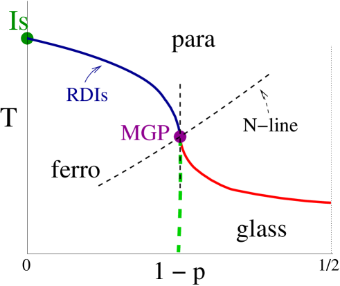
Figure 1: Phase diagram of the three-dimensional $\pm J$ Ising model in the $T$-$p$ plane. The phase diagram is symmetric for $p\rightarrow 1-p$.

The $T$-$p$ phase diagram of the three-dimensional $\pm J$ Ising model is sketched in Fig. 1 for $1\geq p\geq 1/2$ (it is symmetric for $p\rightarrow 1-p$). The high-temperature phase is paramagnetic for any $p$. The nature of the low-temperature phase depends on the value of $p$: it is ferromagnetic for small values of $1-p$, while it is glassy with vanishing magnetization for sufficiently large values of $1-p$. The paramagnetic and low-temperature ferromagnetic and glassy phases are separated by different transition lines, which meet at a magnetic-glassy multicritical point (MGP) located at $p^{*},T^{*}$ and usually called Nishimori point.

The paramagnetic-ferromagnetic (PF) transition line starts from the Ising transition at $p=1$ and extends up to the MGP at $p=p^{*}$. For $p=1$ the transition belongs to the Ising universality class, while for any $1>p>p^{*}$ it belongs to the randomly-dilute Ising (RDIs) universality class,Hukushima-00 ; HPPV-07-pmj characterized by the magnetic critical exponents HPPV-07 ; PV-02 $\nu_{f}=0.683(2)$ and $\eta_{f}=0.036(1)$. The Ising transition at $p=1$ is a multicritical point and, close to it, for $0<1-p\ll 1$, one observes multicritical behaviorHPPV-07-pmj ; CPPV-04 ; Aharony-76 with crossover exponent $\phi=\alpha_{\rm Is}$, whereCPRV-02 $\alpha_{\rm Is}=0.1096(5)$ is the Ising specific-heat exponent. The paramagnetic-glassy (PG) transition line starts from the MGP and extends up to $p=1/2$. A reasonable hypothesis is that the critical behavior is independent of $p$ along the PG line, i.e. that a nonzero average value $[J_{xy}]$ of the bond variables is irrelevant at the glass transition, as found in mean-field models.meanfield Assuming this scenario, for any $1-p^{*}<p<p^{*}$ the PG transition belongs to the same universality class as that of the bimodal Ising spin glass model at $p=1/2$. Its critical behavior has been widely investigated (see, e.g., Refs. KKY-06, ; KR-03, and references therein) and it is characterized by the overlap exponents $\nu_{g}\approx 2.4$ and $\eta_{g}\approx-0.4$.

As argued in Refs. GHDB-85, ; LH-88, ; LH-89, , the MGP is located along the so-called Nishimori line Nishimori-81 ; Nishimori-book (N-line) defined by the relation

$$v\equiv{\rm Tanh}\beta=2p-1,$$ (3)

where $\beta\equiv 1/T$, which allows us to define a Nishimori temperature

$$\beta_{N}(p)={1\over T_{N}(p)}={1\over 2}\ln{p\over 1-p}$$ (4)

for each value of $p$. The $\pm J$ Ising model along the N-line presents several interesting properties. The internal energy has been computed exactly along the N-line:Nishimori-81

$$E_{N}(p)={1\over V}[\langle{\cal H}\rangle_{T_{N}(p)}]=6p-3,$$ (5)

where the angular parentheses and the brackets refer respectively to the thermal average and to the quenched average over the bond couplings $\{J_{xy}\}$. Along the N-line several other remarkable relations hold, such as Nishimori-81

$$[\langle A_{X}\rangle]=[\langle A_{X}\rangle^{2}],$$ (6)

where $A_{X}$ is an arbitrary product of spin variables $\sigma_{x}$, and also LH-88

$$G_{2i+1}(x)=G_{2i+2}(x)\qquad i=1,2,....$$ (7)

where $G_{k}(x)\equiv[\langle\sigma_{0}\,\sigma_{x}\rangle^{k}]$. As a consequence of Eq. (7), the magnetic correlation function $G_{1}(x)$ and the overlap correlation function $G_{2}(x)$ are equal along the N-line. The N-line separates the regions where magnetic and glassy fluctuations dominate. Arguments based on local gauge invariance GHDB-85 ; LH-88 ; LH-89 show that the MGP must be located along the N-line, so that $T^{*}=T_{N}(p^{*})$. At the MGP, magnetic and glassy fluctuations become critical simultaneously.

At fixed $p$ an important inequality holds:Nishimori-81 ; KR-03

$$|[\langle\sigma_{i}\sigma_{j}\rangle_{T}]|\leq[|\langle\sigma_{i}\sigma_{j}\rangle_{T_{N}(p)}|],$$ (8)

where the subscripts indicate the temperature of the thermal average. This relation shows that ferromagnetism can exist only in the region $p>p^{*}$ and that the system is maximally magnetized along the N-line. Ref. Nishimori-86, (see also Refs. Kitatani-92, ; Nishimori-book, ) also reports an argument that indicates that the ferromagnetic-glassy (FG) transition line coincides with the line $p=p^{*}$, from $T=T^{*}$ to $T=0$. This conjecture is contradicted by recent results for the two-dimensional $\pm J$ model WHP-03 ; AH-04 ; PHP-06 and for three-dimensional random-plaquette gauge model, WHP-03 which is the dual of the $\pm J$ model. Violations are in any case quite small. We mention that a mixed low-temperature phase,Kitatani-94 in which ferromagnetism and glass order coexist, is found in mean-field models meanfield such as the infinite-range Sherrington-Kirkpatrick model.SK-75 Its presence has been confirmed in the $\pm J$ Ising model defined on Bethe lattices.CKR-05 However, there is no evidence of this mixed phase in the $\pm J$ Ising model on a cubic lattice Hartmann-99 and in related models.KM-02 Nevertheless, the existence of such a mixed phase is still an open problem, as discussed in Ref. CKR-05, .

In this paper we consider the $\pm J$ model and perform Monte Carlo (MC) simulations along the N-line close to the MGP. By performing a finite-size scaling (FSS) analysis, we locate the multicritical point along the N-line, finding $p^{*}=0.76820(4)$. We determine the renormalization-group (RG) dimensions $y_{1}$ and $y_{2}$ of the relevant operators that control the RG flow close to the MGP and the exponent $\eta$ that gives the critical behavior of the magnetic and of the overlap susceptibility. We obtain $y_{1}=1.02(5)$, $y_{2}=0.61(2)$, and $\eta=-0.114(3)$. The temperature and crossover exponents are $\nu=1/y_{2}=1.64(5)$ and $\phi=y_{2}/y_{1}=1.67(10)$ respectively. We also use our numerical results to estimate the dynamic critical exponent $z$ that characterizes the model-A dynamics HH-77 at the MGP, i.e. a relaxational dynamics without conserved order parameters. We obtain $z=5.0(5)$. Our results significantly improve those obtained in previous works.ON-87 ; Fisch-91 ; Singh-91 ; SA-96 ; MB-98 ; OI-98

The paper is organized as follows. In Sec. II we summarize the theoretical results we need in our numerical analysis. In Sec. III we report our numerical results. We estimate the position of the MGP and the critical exponents $y_{1}$, $y_{2}$, and $\eta$ in Sec. III.1, while in Sec. III.2 we give an estimate of the exponent $z$ for the Metropolis dynamics we use, which is a specific example of a relaxational dynamics without order parameters (the so-called model-A dynamics). In Sec. IV we summarize our results. In the Appendix we report some notations.

II Summary of theoretical results

In the absence of external fields, the critical behavior at the MGP is characterized by two relevant RG operators. The singular part of the free energy averaged over disorder in a volume of size $L$ can be written as

$$F_{\rm sing}(T,p,L)=L^{-d}f(u_{1}L^{y_{1}},u_{2}L^{y_{2}},\{u_{i}L^{y_{i}}\}),\quad i\geq 3,$$ (9)

where $y_{1}>y_{2}>0$, $y_{i}<0$ for $i\geq 3$, $u_{i}$ are the corresponding scaling fields, and $u_{1}=u_{2}=0$ at the MGP. In the infinite-volume limit and neglecting subleading corrections, we have

$$F_{\rm sing}(T,p)=|u_{2}|^{d/y_{2}}f_{\pm}(u_{1}|u_{2}|^{-\phi}),\qquad\phi=y_{1}/y_{2}>1,$$ (10)

where the functions $f_{\pm}(x)$ apply to the parameter regions in which $\pm u_{2}>0$. Close to the MGP, all transition lines correspond to constant values of the product $u_{1}|u_{2}|^{-\phi}$ and thus, since $\phi>1$, they are tangent to the line $u_{1}=0$.

The scaling fields $u_{i}$ are analytic functions of the model parameters $T$ and $p$. Using symmetry arguments, Refs. LH-88, ; LH-89, showed that one scaling axis is along the N-line, i.e. that the N-line is either tangent to the line $u_{1}=0$ or to $u_{2}=0$. Since the N-line cannot be tangent to the transition lines at the MGP and these lines are tangent to $u_{1}=0$, the first possibility is excluded. Thus, close to the MGP the N-line corresponds to $u_{2}=0$. Thus, we identifyLH-88 ; LH-89

$$u_{2}=v-2p+1.$$ (11)

As for the scaling axis $u_{1}=0$, $\epsilon\equiv 6-d$ expansion calculations predict it LH-89 to be parallel to the $T$ axis. The extension of this result to $d=3$ suggests

$$u_{1}=p-p^{*}.$$ (12)

Note that, if Eq. (12) holds, only the scaling field $u_{2}$ depends on the temperature $T$. We may then identify $\nu=1/y_{2}$ as the critical exponent associated with the temperature, and rewrite Eq. (10) as

$$F_{\rm sing}(T,p)=|t|^{d\nu}f_{\pm}(g|t|^{-\phi}),$$ (13)

where $t\equiv(T-T^{*})/T^{*}$, $g\equiv p-p^{*}$, and $\phi$ is the crossover exponent.

These results give rise to the following predictions for the FSS behavior around $T^{*}$, $p^{*}$. Let us consider a RG invariant quantity $R$, such as $R_{\xi}\equiv\xi/L$, $U_{4}$, $U_{22}$, which are defined in the Appendix, and its derivative $R^{\prime}$ with respect to $\beta\equiv 1/T$. In general, in the FSS limit $R$ obeys the scaling law

$$R={\cal R}(u_{1}L^{y_{1}},u_{2}L^{y_{2}},\{u_{i}L^{y_{i}}\}),\quad i\geq 3.$$ (14)

Neglecting the scaling corrections, that is terms vanishing in the limit $L\to\infty$, close to the MGP we expect

$$R=R^{*}+b_{11}u_{1}L^{y_{1}}+b_{21}u_{2}L^{y_{2}}+\ldots.$$ (15)

which is valid as long as $u_{1}L^{y_{1}}$ is small. Along the N-line, the scaling field $u_{2}$ vanishes, so that we can write

$$R_{N}=R^{*}+b_{11}u_{1}L^{y_{1}}+\ldots,$$ (16)

where the subscript $N$ indicates that $R$ is restricted to the N-line. Let us now consider the derivative of $R$ with respect to $\beta$. Differentiating Eq. (15), we obtain

$$R^{\prime}=b_{11}u^{\prime}_{1}L^{y_{1}}+b_{21}u^{\prime}_{2}L^{y_{2}}+\cdots$$ (17)

If Eq. (12) holds, then $u^{\prime}_{1}=0$, so that

$$R^{\prime}=b_{21}u^{\prime}_{2}L^{y_{2}}+\cdots$$ (18)

This result gives us a method to verify the conjecture of Ref. LH-89, : once $y_{1}$ has been determined from the scaling behavior of a RG invariant ratio close to the MGP, it is enough to check the scaling behavior of $R^{\prime}$. If $R^{\prime}$ scales as $L^{x}$ with $x<y_{1}$, the conjecture is confirmed and $x$ provides an estimate of $y_{2}$.

Finally, we consider the magnetic susceptibility. Along the N-line it behaves as

$$\chi_{N}=eL^{2-\eta}\left(1+e_{1}u_{1}L^{y_{1}}+\cdots\right).$$ (19)

Note that there is only one $\eta$ exponent which characterizes the critical behavior of both the magnetic and overlap correlation functions,LH-88 since they are equal along the N-line, see Eq. (7).

III Results

In the following we present a FSS analysis of high-statistics MC data along the N-line close to the MGP. We performed MC simulations for lattice sizes $L=8,12,16,24,32$, taking periodic boundary conditions. We used a standard Metropolis algorithm and multispin coding (details can be found in Ref. HPPV-07-pmj, ). Most of the simulations correspond to values of $p$ in the range $0.7680\leq p\leq 0.7685$, i.e. very close to the MGP, which, as we show below, is located at $p^{*}=0.76820(4)$: typically, we considered 6 values of $p$ in this range for each value of $L$. To obtain small statistical errors, we generated a large number of samples: $2\times 10^{5}$ for $L\leq 16$, $10^{5}$ for $L=24$, and $4\times 10^{4}$ for $L=32$. Because of the long equilibration times, for each sample we performed a large number of Metropolis sweeps; for $L=16$, 24, 32, the number of sweeps is $10^{6}$, $8\times 10^{6}$, and $5\times 10^{7}$, respectively. To guarantee equilibration, typically 30% of the data were discarded (but, for $L=32$, we discarded 50% of the data). All MC data are available on request. Below we report the results of the analyses: in Sec. III.1 we consider the static exponents, while in Sec. III.2 we focus on the dynamics.

III.1 Static exponents

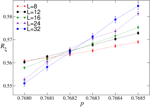
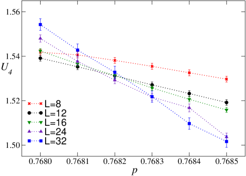
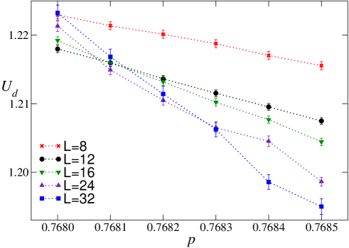
Figure 2: MC data of $R_{\xi}\equiv\xi/L$, $U_{4}$, and $U_{d}$ vs $p$.

MC estimates of the RG invariant quantities $R_{\xi}$, $U_{4}$, and $U_{d}$ along the N-line are shown in Fig. 2. There is clearly a crossing point at $p\approx 0.7682$, which provides a first rough estimate of the location of the MGP point. In order to estimate precisely $p^{*}$, $T^{*}$, and $y_{1}$ we fit the renormalized couplings $R$ close to the MGP to

$$R=R^{*}+a(\beta-\beta^{*})L^{y_{1}},$$ (20)

keeping $R^{*}$, $\beta^{*}$, and $y_{1}$ as free parameters. Note that this functional form relies on the property that $u_{2}=0$ along the N-line. Otherwise, an additional term of the form $(\beta-\beta^{*})L^{y_{2}}$ should be added. We also neglect scaling corrections that behave as $cL^{y_{3}}$ with $y_{3}<0$. Indeed, since we only have data in a limited range of values of $L$, we are not able to include reliably a correction of this type.

	$\chi^{2}$/DOF	$\beta^{*}$	$y_{1}$	$U_{22}^{*}$	$R_{\xi}^{*}$
$U_{22},R_{\xi}$	0.88	0.59910(2)	1.02(5)	$0.3180(3)$	0.5648(3)
$U_{22},R_{\xi},U_{d}$	1.43	0.59902(2)	1.02(4)	$0.3189(3)$	0.5640(4)	$U_{d}^{*}=1.2137(3)$
$U_{22},R_{\xi},U_{4}$	0.62	0.59914(2)	1.01(5)	$0.3178(3)$	0.5656(4)	$U_{4}^{*}=1.5302(6)$

Table 1: Results of combined fits. The first fit uses all data with $L\geq 8$, the last two fits only those with $L\geq 12$. DOF is the number of degrees of freedom of the fit.

	$L_{\rm min}$	$\chi^{2}$/DOF	$\beta^{*}$	$x$
$R_{\xi},R_{\xi}^{\prime}$	8	0.92	0.59905(3)	0.600(2)
	12	0.70	0.59912(3)	0.609(4)
	16	0.64	0.59910(4)	0.604(7)
$U_{22},R_{\xi}^{\prime}$	8	0.69	0.59929(6)	0.602(2)
	12	0.55	0.59936(7)	0.611(4)
	16	0.46	0.59934(10)	0.607(7)
$R_{\xi},U_{4}^{\prime}$	8	2.06	0.59907(3)	0.579(3)
	12	0.71	0.59912(3)	0.611(5)
	16	0.60	0.59910(4)	0.619(9)
$U_{22},U_{4}^{\prime}$	8	1.60	0.59937(6)	0.569(3)
	12	0.55	0.59936(6)	0.601(6)
	16	0.43	0.59934(10)	0.607(10)

Table 2: Estimates of $x$. We report results obtained by analyzing simultaneously two different quantities and including only data satisfying $L\geq L_{\rm min}$. DOF is the number of degrees of freedom of the fit.

Fits that involve $R_{\xi}$ and $U_{22}$ have an acceptable $\chi^{2}$ even if we include all data with $L\geq 8$: there is no evidence of scaling corrections. On the other hand, in fits of $U_{4}$ or $U_{d}$ the data with $L=8$ must be discarded to obtain a good $\chi^{2}$. To obtain more accurate estimates, we have performed combined fits in which several RG invariant quantities are fitted together. The results are reported in Table 1. The dependence on the observables used in the fit is reasonably small and allows us to estimate

$$\beta^{*}=0.5991(1),$$ (21)

$$y_{1}=1.02(5).$$ (22)

The errors take into account the variation of the estimates with the different observables used in the fits (note that statistical errors are much smaller). Since scaling corrections are expected to differ in the different observables, this should allow us to take indirectly into account the scaling corrections. We have then $T^{*}=1/\beta^{*}=1.6692(3)$, and, by using Eq. (3),

$$p^{*}=0.76820(4).$$ (23)

In Table 1 we also report estimates of the critical value of the RG renormalized couplings. Note that $U_{22}^{*}\approx 0.318$, which is significantly higher than the corresponding result for the RDIs universality class, $U_{22}^{*}=0.1479(6)$.HPPV-07 This indicatesAH-96 that the violations of self-averaging are much stronger at the MGP than along the PF transition line, as of course should be expected.

We consider now the derivative $R^{\prime}$ of the RG invariant quantities with respect to $\beta$. They have been determined by considering the connected correlations of $R$ and of the Hamiltonian. At the critical point, $R^{\prime}$ is expected to behave as $L^{x}$ for large $L$, where $x=y_{2}$, if the argument of Ref. LH-89, holds; otherwise, one should have $x=y_{1}$. In order to determine $x$, we fit $\ln R^{\prime}$ to

$$\ln R^{\prime}=a+x\ln L+b(\beta-\beta^{*})L^{y_{1}},$$ (24)

keeping $y_{1}$ fixed to $y_{1}=1.02(5)$. To avoid fixing $\beta_{c}$ we perform combined fits in which one derivative $R^{\prime}_{1}$ and one RG coupling $R_{2}$ are fitted together. The results are reported in Table 2. The $\chi^{2}$ of the fit is always good except when we use $L_{\rm min}=8$ and $U_{4}^{\prime}$. If we do not consider the corresponding results, all estimates of $x$ are close to $0.61$. Analyses of $R^{\prime}_{\xi}$ are apparently stable with $L_{\rm min}$, while those of $U^{\prime}_{4}$ show a slight upward trend. A reasonable final estimate is $x=0.61(2)$, which takes into account all results with their error bars. This result is significantly different from $y_{1}$ and thus confirms the argument of Ref. LH-89, . Since $x<y_{1}$, $x$ should be identified with $y_{2}$. Therefore, we obtain the estimates

$$y_{2}=0.61(2),\qquad\qquad\nu={1\over y_{2}}=1.64(5).$$ (25)

The crossover exponent is therefore

$$\phi={y_{1}\over y_{2}}=1.67(10).$$ (26)

The same analysis used to estimate $y_{2}$ can be employed to determine $\eta$. Instead of $\chi$, we consider the ratio $Z\equiv\chi/\xi^{2}$, which has smaller statistical errors. Since $Z\sim L^{-\eta}$ for $L\to\infty$ at the critical point, we fit the MC data to

$$\ln Z=a-\eta\ln L+b(\beta-\beta^{*})L^{y_{1}}.$$

As before, we fix $y_{1}$ and perform combined fits of $\ln Z$ with a RG invariant coupling, considering only data satisfying $L\geq L_{\rm min}$. Fits of $Z$ and $R_{\xi}$ give $\eta=-0.1155(6)$ and $-0.1154(9)$ for $L_{\rm min}=8,12$; if we use $U_{22}$ instead of $R_{\xi}$, we obtain $\eta=-0.1134(7)$ and $-0.1131(9)$ for $L_{\rm min}=8,12$. The $L_{\rm min}$ dependence is small and results change only slightly with the observable. We take as our final estimate

$$\eta=-0.114(3).$$ (27)

Our FSS results significantly improve earlier results. Ref. Singh-91, reports the computation and analysis of the 34th-order high-temperature (HT) series of some susceptibilities

$$\chi_{m,n}={1\over V}\sum_{ij}[\langle s_{i}s_{j}\rangle^{m}]^{n}$$ (28)

along the N-line, obtaining $p^{*}=0.7656(20)$, $y_{1}=1.18(11)$, $\phi\equiv y_{1}/y_{2}=1.85(14)$, $\eta=-0.10(2)$. These estimates are substantially consistent with ours. As a further check, we reanalize the 34th-order HT series reported in Ref. Singh-91, , by biasing the value of the critical point with the MC estimate (21). Using biased first-order integral approximants, see, e.g., Ref. CPRV-02, for details, we obtain $(2-\eta)/y_{1}=2.08(7)$ from the series of $\chi_{11}$, $(1-2\eta)/y_{1}=1.25(17)$ from the series of $\chi_{22}$, $3/y_{1}=3.03(14)$ from the series of the ratio $\chi_{11}^{2}/\chi_{22}$, and $(2-\eta-y_{2})/y_{1}=2.70(9)$ from $v\partial\chi_{21}/\partial v$, from which we can derive the estimates $y_{1}=0.99(5)$, $\phi\equiv y_{1}/y_{2}=1.6(3)$, and $\eta=-0.1(1)$, which are in good agreement with our FSS results.

Other results can be found in Refs. ON-87, ; Fisch-91, ; MB-98, ; they are apparently less precise and not consistent with ours within the reported errors. For example, we mention the recent estimates $p^{*}=0.7673(3)$ obtained by off-equilibrium MC simulationsOI-98 and $p^{*}\approx 0.622$ obtained by a RG study.MB-98 Note that estimate (23) and the conjecturefootnote of Refs. TSN-05, ; Nishimori-07, allow us to find the location of the multicritical point that occurs in the three-dimensional random-plaquette gauge model. We obtain $p^{*}_{\rm gauge}=0.9650(1)$, which is in agreement with, though much more precise than, the result of Ref. OAIM-04, , $p^{*}_{\rm gauge}=0.967(4)$.

III.2 Model-A dynamic exponent $z$

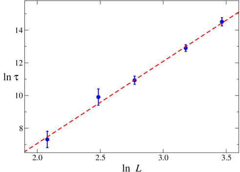
Figure 3: Estimates of the exponential autocorrelation time $\tau$ at the MGP vs $L$.

Finally, we present some results on the dynamic behavior of the Metropolis algorithm, which represents a particular implementation of a relaxational dynamics without conserved order parameters (model-A dynamics).HH-77 Note that at the MGP there is only one dynamic exponent $z$ characterizing the relaxation of both the magnetic and the glassy critical modes, since their autocorrelation functions are strictly equal along the N-line.OI-98 In Fig. 3 we show estimates of the exponential autocorrelation time $\tau$ at the MGP as extracted from the connected autocorrelation function of the magnetic susceptibility

$$G_{\chi}(t_{1}-t_{2})\equiv\left[{\langle\chi(t_{1})\chi(t_{2})\rangle_{c}}\right].$$ (29)

For large $L$ and $T=T^{*}$, $\tau$ is expected to scale as $L^{z}$, where $z$ is the dynamic critical exponent. A linear fit of the MC results to $\ln\tau=a+b\ln L$ gives the estimate $z=5.0(5)$, which is significantly larger than the value at the PF transition line $z=2.35(2)$.HPV-07 Instead this estimate is close to the value of $z$ obtained for the bimodal Ising spin-glass model, $z=5.7(2)$.PC-05

We also determine the exponent $\lambda$ which describes the nonequilibrium relaxation of the magnetization at $T_{c}$ from a starting configuration in which all spins are parallel.OI-98 Asymptotically, for $t\rightarrow\infty$, one expects

$$M(t)\sim t^{-\lambda},\qquad\lambda={1+\eta\over 2z},$$ (30)

see, e.g., Ref. OI-98, and references therein. Our results lead to the estimate $\lambda=0.09(1)$, which is perfectly consistent with the estimate OI-98 $\lambda=0.090(3)$ obtained in off-equilibrium MC simulations.

IV Conclusions

In this paper we have considered the critical behavior close to the MGP which is present in the phase diagram of the $\pm J$ model. Our main results are the following:

• We have obtained an accurate estimate of the location of the MGP: $p^{*}=0.76820(4)$, $\beta^{*}=0.5991(1)$. It is worth observing that our estimate of $p^{*}$ is very close to the result Hartmann-99 $p_{c}=0.778(5)$ for the location of the FG transition at $T=0$ and satisfies the rigorous inequality $p_{c}\geq p^{*}$ which follows from Eq. (8). Our results show therefore that, even if the conjectureNishimori-86 ; Kitatani-92 that the FG transition line does not depend on the temperature is not true, deviations are quite small.

• We have verified the conjecture of Ref. LH-89, : the scaling field $u_{1}$ associated with the RG operator with the largest RG dimension does not depend on the temperature.

• We have determined the critical exponents $y_{1}=1.02(5)$, $y_{2}=0.61(2)$, $\nu\equiv 1/y_{2}=1.64(5)$, $\phi\equiv y_{1}/y_{2}=1.67(10)$, and $\eta=-0.114(3)$.

• We have determined the dynamic critical exponent $z$ associated with the model-A dynamics, obtaining $z=5.0(5)$.

Our results are significantly more precise than those obtained in previous works.ON-87 ; Fisch-91 ; Singh-91 ; SA-96 ; MB-98 ; OI-98 They can be used to explain experiments on materials containing both ferromagnetic and antiferromagnetic ions. An example is Fe_xMn_1-xTiO₃, which shows Ising behavior for $x=1$ and $x=0$, a PG transition for $0.38\lesssim x\lesssim 0.58$ and a PF transition for $0<x\lesssim 0.38$ and $0.58\lesssim x<1$.YMAI-89 ; AKI-93 The MGP should be located at $x\approx 0.38$ and at $x\approx 0.58$. Close to these values our results apply.

Appendix A Notations

Setting

$$G_{k}(x)\equiv[\langle\sigma_{0}\,\sigma_{x}\rangle^{k}],$$ (31)

where the angular parentheses and the brackets indicate respectively the thermal average and the quenched average over $J_{xy}$, the magnetic and overlap correlation functions are given respectively by $G_{1}(x)$ and $G_{2}(x)$. Along the N-line, cf. Eq. (3), $G_{1}(x)=G_{2}(x)$.

We define the magnetic susceptibility $\chi\equiv\sum_{x}G_{1}(x)$ and the correlation length $\xi$

$$\xi^{2}\equiv{\widetilde{G}_{1}(0)-\widetilde{G}_{1}(q_{\rm min})\over\hat{q}_{\rm min}^{2}\widetilde{G}_{1}(q_{\rm min})},$$ (32)

where $q_{\rm min}\equiv(2\pi/L,0,0)$, $\hat{q}\equiv 2\sin q/2$, and $\widetilde{G}_{1}(q)$ is the Fourier transform of $G_{1}(x)$. We also consider quantities that are invariant under RG transformations in the critical limit. Beside the ratio

$$R_{\xi}\equiv\xi/L,$$ (33)

we consider the quartic cumulants $U_{4}$, $U_{22}$, and $U_{d}$ defined by

$$U_{4}\equiv{[\mu_{4}]\over[\mu_{2}]^{2}},$$ (34)

$$U_{22}\equiv{[\mu_{2}^{2}]-[\mu_{2}]^{2}\over[\mu_{2}]^{2}},$$

$$U_{d}\equiv U_{4}-U_{22},$$

where

$$\mu_{k}\equiv\langle\;(\sum_{x}\sigma_{x}\;)^{k}\rangle\;.$$ (35)

Analogous quantities $R^{o}_{\xi}$, $U^{o}_{4}$, $U^{o}_{22}$, and $U^{o}_{d}$ can be defined by using the overlap variable $q_{x}\equiv\sigma_{x}^{(1)}\sigma_{x}^{(2)}$, where the superscripts indicate two independent configurations for given disorder. Using Eq. (6), one can easily check that along the N-line $R_{\xi}=R^{o}_{\xi}$ and $U_{4}=U^{o}_{4}$. This implies that also their fixed-point values are the same at the MGP.

Finally, we consider the derivatives

$$R^{\prime}_{\xi}\equiv{dR_{\xi}\over d\beta},\qquad U^{\prime}_{4}\equiv{dU_{4}\over d\beta},$$ (36)

which can be computed by measuring appropriate expectation values at fixed $\beta$ and $p$.

References

- (1) S. F. Edwards and P. W. Anderson, J. Phys. F 5, 965 (1975).
- (2) A. Ito, H. Aruga, E. Torikai, M. Kikuki, Y. Syono, and H. Takei, Phys. Rev. Lett. 57, 483 (1986).
- (3) K. Gunnarsson, P. Svedlindh, P. Nordblad, L. Lundgren, H. Aruga, and A. Ito, Phys. Rev. B 43, 8199 (1991).
- (4) S. Nair and A. K. Nigam, Phys. Rev. B 75, 214415 (2007).
- (5) K. Hukushima, J. Phys. Soc. Japan 69, 631 (2000).
- (6) M. Hasenbusch, F. Parisen Toldin, A. Pelissetto, and E. Vicari, Phys. Rev. B 76, (2007) [arXiv:cond-mat/0704.0427].
- (7) M. Hasenbusch, F. Parisen Toldin, A. Pelissetto, and E. Vicari, J. Stat. Mech.: Theory Expt. P02016 (2007).
- (8) A. Pelissetto and E. Vicari, Phys. Rept. 368, 549 (2002).
- (9) P. Calabrese, P. Parruccini, A. Pelissetto, and E. Vicari, Phys. Rev. E 69, 036120 (2004).
- (10) A. Aharony, in Phase Transitions and Critical Phenomena, Vol. 6, edited by C. Domb and M.S. Green (Academic Press, New York, 1976), p. 357.
- (11) M. Campostrini, A. Pelissetto, P. Rossi, and E. Vicari, Phys. Rev. E 65, 066127 (2002).
- (12) G. Toulouse, J. Physique Lettres 41, 447 (1980).
- (13) H. Katzgraber, M. Körner, and A. P. Young, Phys. Rev. B 73, 224432 (2006).
- (14) N. Kawashima and H. Rieger, in Frustrated Spin Systems, edited by H.T. Diep (World Scientific, Singapore, 2004); cond-mat/0312432.
- (15) A. Georges, D. Hansel, P. Le Doussal, and J. Bouchaud, J. Phys. (Paris) 46, 1827 (1985).
- (16) P. Le Doussal and A. B. Harris, Phys. Rev. Lett. 61, 625 (1988).
- (17) P. Le Doussal and A. B. Harris, Phys. Rev. B 40, 9249 (1989).
- (18) H. Nishimori, Prog. Theor. Phys. 66, 1169 (1981).
- (19) H. Nishimori, Statistical Physics of Spin Glasses and Information Processing: An Introduction (Oxford University Press, Oxford, 2001).
- (20) H. Nishimori, J. Phys. Soc. Japan 55, 3305 (1986).
- (21) H. Kitatani, J. Phys. Soc. Japan 61, 4049 (1992).
- (22) C. Wang, J. Harrington, and J. Preskill, Ann. Phys. 303, 31 (2003).
- (23) C. Amoruso and A. K. Hartmann, Phys. Rev. B 70, 134425 (2004).
- (24) M. Picco, A. Honecker, and P. Pujol, J. Stat. Mech.: Theory Expt. P09006 (2006).
- (25) It can be shown rigorously that the N-line never intersects the spin-glass phase, H. Kitatani, J. Phys. Soc. Japan 63, 2070 (1994). Since we must also have , the mixed phase, if it exists, should be confined to the region below the N-line and on the left of the line (see Fig. 1).
- (26) D. Sherrington and S. Kirkpatrick, Phys. Rev. Lett. 35, 1792 (1975).
- (27) T. Castellani, F. Krzakala, and F. Ricci Tersenghi, Eur. Phys. J. B 47, 99 (2005).
- (28) A. K. Hartmann, Phys. Rev. B 59, 3617 (1999).
- (29) F. Krzakala and O.C. Martin, Phys. Rev. Lett. 89, 267202 (2002).
- (30) P. C. Hohenberg and B. I. Halperin, Rev. Mod. Phys. 49, 435 (1977).
- (31) Y. Ozeki and H. Nishimori, J. Phys. Soc. Japan 56, 1568 (1987); J. Phys. Soc. Japan 56, 3265 (1987).
- (32) R. Fisch, Phys. Rev. B 44, 652 (1991).
- (33) R. R. P. Singh, Phys. Rev. Lett. 67, 899 (1991).
- (34) R. R. P. Singh and J. Adler, Phys. Rev. B 54, 364 (1996).
- (35) G. Migliorini and A. N. Berker, Phys. Rev. B 57, 426 (1998).
- (36) Y. Ozeki and N. Ito, J. Phys. A 31, 5451 (1998).
- (37) A. Aharony and A. B. Harris, Phys. Rev. Lett. 77, 3700 (1996).
- (38) Note that the duality relations reported in Ref. TSN-05, are not rigorous. Numerical results are generically consistent (see Table I in Ref. Nishimori-07, ), even though tiny discrepancies have been observed in several cases.
- (39) K. Takeda, T. Sasamoto, and H. Nishimori, J. Phys. A 38, 3751 (2005).
- (40) H. Nishimori, J. Stat. Phys. 126, 977 (2007).
- (41) T. Ohno, G. Arakawa, I. Ichinose, and T. Matsui, Nucl. Phys. B 697, 462 (2004).
- (42) M. Hasenbusch, A. Pelissetto, and E. Vicari, in preparation.
- (43) M. Pleimling and I. A. Campbell, Phys. Rev. B 72, 184429 (2005).
- (44) H. Yoshizawa, S. Mitsuda, H. Aruga, and A. Ito, J. Phys. Soc. Jpn. 58, 1416 (1989).
- (45) H. Aruga Katori and A. Ito, J. Phys. Soc. Jpn. 62, 4488 (1993).