XMM-Newton observations of the Lockman Hole V: time variability of the brightest AGN

This paper presents the results of a study of X-ray spectral and flux variability on time scales from months to years, of the 123 brightest objects (including 46 type-1 AGN and 28 type-2 AGN) detected with XMM-Newton in the Lockman Hole field. We detected flux variability with a significance $\geq$3$\sigma$ in $\sim$50% of the objects, including 68$\pm$11% and 48$\pm$15% among our samples of type-1 and type-2 AGN. However we found that the fraction of sources with best quality light curves that exhibit flux variability on the time scales sampled by our data is $\geq 80\%$, i.e the great majority of the AGN population may actually vary in flux on long time scales. The mean relative intrinsic amplitude of flux variability was found to be $\sim$0.15 although with a large dispersion in measured values, from $\sim$0.1 to $\sim$0.65. The flux variability properties of our samples of AGN (fraction of variable objects and amplitude of variability) do not significantly depend on the redshift or X-ray luminosity of the objects and seem to be similar for the two AGN types. Using a broad band X-ray colour we found that the fraction of sources showing spectral variability with a significance $\geq$3$\sigma$ is $\sim$40% i.e. less common than flux variability. Spectral variability was found to be more common in type-2 AGN than in type-1 AGN with a significance of more than 99%. This result is consistent with the fact that part of the soft emission in type-2 AGN comes from scattered radiation, and this component is expected to be much less variable than the hard component. The observed flux and spectral variability properties of our objects and especially the lack of correlation between flux and spectral variability in most of them cannot be explained as being produced by variability of one spectral component alone, for example changes in $\Gamma$ associated with changes in the mass accretion rate, or variability in the amount of X-ray absorption. At least two spectral components must vary in order to explain the X-ray variability of our objects.

1 Introduction

Active Galactic Nuclei (AGN) are strongly variable sources in all wave bands (Edelson et al. Edelson96 (1996); Nandra et al. Nandra98 (1997)) and on different time scales. The largest amplitude and fastest variability is usually observed in X-rays. This is taken as evidence for X-ray emission in AGN originating in a small region close to the central object, which is thought to be a supermassive ($10^{6}-10^{9}{\rm M_{\odot}}$) black hole.

It has been found that AGN are generally more variable on long time scales than on short time scales (see Barr & Mushotzky Barr86 (1986); Nandra et al. Nandra97 (1997); Markowitz & Edelson Markowitz01 (2001)). In addition, it is well known that variability amplitude on short (Barr & Mushotzky Barr86 (1986); Nandra et al. Nandra97 (1997); Turner et al. Turner99 (1999); Lawrence & Papadakis Lawrence93 (1993)) and long (Markowitz & Edelson Markowitz01 (2001)) time scales, when measured over a fixed temporal frequency, is anti-correlated with the X-ray luminosity, i.e. lower variability amplitudes are seen in more luminous sources. All these results are consistent with recent results based on power spectrum analysis of light curves of AGN (Markowitz et al. 2003a ; McHardy et al. McHardy06 (2006)). There are also indications that the strength of the anti-correlation might decrease towards longer time scales (Markowitz et al. Markowitz04 (2004)).

All these findings are consistent with a scenario where more luminous sources, hosting more massive black holes, have larger X-ray emitting regions, and therefore the variability needs more time to propagate through the X-ray emitting region.

X-ray spectral variability studies of nearby objects have shown that most AGN tend to become softer when they brighten (see e.g. Markowitz et al. 2003b ; Nandra et al. Nandra97 (1997)) similar to the different flux-spectral states seen in black hole X-ray binaries (BHXRB) (McClintock et al. McClintock03 (2003)). In addition, nearly all AGN exhibit stronger variability at soft X-rays on all time scales (Markowitz et al. Markowitz04 (2004)).

Two phenomenological model parameterisations have been proposed to explain the variability patterns observed in AGN (see e.g. Taylor et al. Taylor03 (2003)): in the two-component spectral model (${\rm M^{c}}$Hardy et al. McHardy98 (1998), Shih et al. Shih02 (2002)) a softer continuum emission power law component of constant slope but variable flux (probably associated with the emission from the hot corona) is superimposed on a harder spectral component with constant flux (likely associated with the Compton reflection hump). This model does not require the form of any of the spectral components to vary, what varies is the relative contribution of the soft and hard spectral components with time. When the source becomes brighter the soft component dominates the spectrum and the source becomes softer. In the two-component spectral model it is expected that as the sources become brighter their X-ray spectral slope will saturate to the slope of the soft component. However, some bright objects show evidence for variations in their underlying continuum spectrum (e.g. NGC 4151 see Perola et al. Perola86 (1986); Yaqoob & Warwick Yaqoob91 (1991); Yaqoob et al. Yaqoob93 (1993)). For these objects the two component spectral model cannot explain their variability properties.

An alternative parameterisation is the spectral pivoting model: in this model flux-correlated changes in the continuum shape are due to changes in a single variable component, that becomes softer as the source brightens (see e.g. Zdziarski et al. Zdziarski03 (2003)).

Although X-ray spectral variability in a significant number of AGN can be explained as due to changes in the primary continuum shape, changes in the column density of the cold gas responsible for the absorption in X-rays have been reported on time-scales of months-years in both type-1 and type-2 Seyfert galaxies (Risaliti et al. Risaliti02 (2002); Malizia et al. Malizia97 (1997); Puccetti et al. Puccetti04 (2004)). The absorbing material in these objects must be clumpy and due to the time scales involved, it must be close to the central black hole, much nearer than the standard torus of AGN unification models (Antonucci et al. Antonucci93 (1993)).

Table 1: Summary of XMM-Newton EPIC-pn observations in the Lockman Hole.

Rev/ObsId	obs phase	R.A.	Dec	obs. date	${\rm Filter}$	${\rm GTI}$
(1)	(2)	(3)	(4)	(5)	(6)	(7)
070 / 0123700101	PV	10  52  43.0	+57  28  48	2000-04-27	Th	34
073 / 0123700401	PV	10  52  43.0	+57  28  48	2000-05-02	Th	14
074 / 0123700901	PV	10  52  41.8	+57  28  59	2000-05-05	Th	5
081 / 0123701001	PV	10  52  41.8	+57  28  59	2000-05-19	Th	27
345 / 0022740201	AO1	10  52 43.0	+57  28  48	2001-10-27	M	40
349 / 0022740301	AO1	10  52 43.0	+57  28  48	2001-11-04	M	35
522 / 0147510101	AO2	10  51  03.4	+57  27  50	2002-10-15	M	79
523 / 0147510801	AO2	10  51  27.7	+57  28  07	2002-10-17	M	55
524 / 0147510901	AO2	10  52  43.0	+57  28  48	2002-10-19	M	55
525 / 0147511001	AO2	10  52  08.1	+57  28  29	2002-10-21	M	78
526 / 0147511101	AO2	10  53  17.9	+57  29  07	2002-10-23	M	45
527 / 0147511201	AO2	10  53  58.3	+57  29  29	2002-10-25	M	30
528 / 0147511301	AO2	10  54  29.5	+57  29  46	2002-10-27	M	28
544 / 0147511601	AO2	10  52  43.0	+57  28  48	2002-11-27	M	104
547 / 0147511701	AO2	10  52  40.6	+57  28  29	2002-12-04	M	98
548 / 0147511801	AO2	10  52  45.3	+57  29  07	2002-12-06	M	86

Columns are as follows: (1) XMM-Newton revolution and observation identifier; (2) Observation phase: Verification Phase (PV), first and second announcements of opportunity (AO1 and AO2); (3) and (4) pointing coordinates in right ascension and declination (J2000); (5) Observation date; (6) and (7) EPIC-pn blocking filter^a of the observation and good time interval (in ksec) after subtracting periods of the observation affected by high background flares.
^a Blocking filters: Th: Thin at 40nm A1; M: Medium at 80nm A1.

In this paper we present the results of a study of the flux and spectral variability properties of the 123 brightest objects detected with XMM-Newton in the Lockman Hole field, for which their time-averaged X-ray spectral properties are known, and were presented in a previous paper (Mateos et al. 2005b ). The aim of this study is to provide further insight into the origin of the X-ray emission in AGN, by analysing the variability properties of the objects on long time scales, from months to years. It is important to note that the variability analysis presented here does not allow us to study, for example, fluctuations in the accretion disc, as the dynamical time scales (light-crossing time) are much shorter than the ones sampled in our analysis. Intra-orbit variability studies (i.e. on time scales $<$2 days) cannot be performed on the Lockman Hole sources, as they are too faint. With our analysis we can detect, for example, variability related to changes in the global accretion rate, such as variations in the accretion rate propagating inwards (Lyubarskii Lyubarskii97 (1997)). In addition, we can investigate whether the detected long-term X-ray variability in our objects can be explained as being due to variations in the obscuration of the nuclear engine.

This paper is organised as follows: Sec. 2 describes the X-ray data that was used for the analysis and explains how we built our sample of objects; in Sec. 3 we describe the approach that we followed to carry out our variability analysis; the results of the study of flux and spectral variability in our objects are shown in Sec. 4 and Sec. 5; Sec. 6 explores the true fraction of sources where either flux or spectral variability are present; a discussion of the results and possible interpretations for the origin of the long-term variability are presented in Sec. 7; Sec. 8 presents the variability properties of the type-2 AGN in our sample without any sign of X-ray absorption in their co-added X-ray spectra; finally the results of our analysis are summarised in Sec. 9.

Throughout this paper we have adopted the WMAP concordance cosmology model parameters (Spergel et al. Spergel03 (2003)) with ${\rm H_{0}=70\,km\,s}^{-1}\,{\rm Mpc}^{-1}$, $\Omega_{M}=0.3$ and $\Omega_{\Lambda}=0.7$.

2 XMM-Newton deep survey in the Lockman Hole

The XMM-Newton observatory has carried out its deepest observation in the direction of the Lockman Hole field, centred at R.A.:10:52:43 and Dec:+57:28:48 (J2000). The XMM-Newton deep survey in the Lockman Hole is composed of 16 observations carried out from 2000 to 2002, which allow us to study the X-ray variability properties of our sources on long time scales, from months to years. The Lockman Hole was also observed during revolutions 071 ($\sim$61 ksec) and 344 ($\sim$80 ksec duration). However at the time of this analysis there was no Observation Data File (ODF) available for the observation in revolution 071, and hence, we could not use that data. We could not use the data from revolution 344 because most of the observation was affected by high and flaring background. We report the summary of the XMM-Newton observations in the Lockman Hole used in our study in Table 1. The first column shows the revolution number and observation identifier. The second column shows the name of the phase of observation (PV for observations during the Payload Verification Phase, and AO1 and AO2 for observations during the first and second Announcements of Opportunity). The third and fourth columns list the pointing coordinates of the observation. Column five lists the observation dates, while the last two columns show the filters that were used during each observation for the EPIC-pn X-ray detector, together with the exposure times after removal of periods of high background. The 16 XMM-Newton observations gave a total exposure time (after removal of periods of high background) of $\sim$650 ksec for the EPIC-pn data.

2.1 Sample of sources

A detailed description of how the list of XMM-Newton detected sources in the total observation of the Lockman Hole was obtained can be found in Mateos et al.( 2005b ). In brief, the XMM-Newton Science Analysis Software (SAS, Gabriel et al. Gabriel2004 (2004)) was used to analyse the X-ray data. The event files of each observation were filtered to remove periods of time affected by high background. Images, exposure maps and background maps were obtained for each individual observation and for the EPIC-pn detector on the five standard XMM-Newton energy bands (0.5-2, 2-4.5, 4.5-7.5, 7.5-12 keV). The data were summed to obtain the total observation of the field for each energy band. The SAS source detection algorithm eboxdetect-emldetect was run on the five XMM-Newton energy bands simultaneously to produce an X-ray source list for the total observation.

From the final list of sources the 123 brightest objects (with more than 500 source-background subtracted 0.2-12 keV counts) were selected for analysis. Because the main goal was to study the X-ray properties of AGN, objects identified as clusters of galaxies or stars were excluded from the sample. At the time of the analysis, 74 ($\sim$ 60%) of the selected objects had optical spectroscopic identifications available. Of these, 46 were optically classified as type-1 AGN and 28 as type-2 AGN.

3 X-ray variability analysis

The three XMM-Newton EPIC cameras (M1, M2 and pn) have different geometries, therefore for a given observation, it is common to find that a significant number of serendipitously detected objects fall near or inside CCD gaps in at least one of the cameras. This means that, for the same object, we will have light curves from different data sets (i.e. data from different revolutions) for each camera and therefore the sampling is different. In addition, because of their different instrumental responses we cannot combine the count rates from the three EPIC cameras. The fact that light curves from each EPIC camera are sampled differently in most sources, makes comparing the results of our variability analysis between detectors very difficult. Due to the geometry of the pn detector, the number of sources falling in the pn CCD gaps will be larger than in MOS detectors; however the former provides the deepest observation of the field for each exposure, which allows us to detect lower variability amplitudes, and to measure better the variability amplitude. Therefore, we have used only pn data in the analysis presented in this paper. The pn source lists obtained for each revolution were visually screened to remove spurious detections of hot pixels still present in the X-ray images.

Source detection was carried out on the EPIC-pn data from each individual revolution to obtain all the relevant parameters for the selected sources from all observations where they were detected. We have used measured 0.2-12 keV count rates from each individual observation where sources were detected, to build light curves.

Source parameters become very uncertain for objects detected close to CCD gaps. To avoid this problem, we did not use data from observations where the objects were detected near CCD gaps, bad columns, or near the edge of the Field of View (FOV). To remove these cases we created detector masks, one for each observation, increasing the size of the CCD gaps up to the radius that contains 80% of the telescope PSF on each detector point. We used these masks to remove automatically non desired data.

Each point on the light curves corresponds to the average count rate of the sources in that revolution. The exposure times of the EPIC-pn observations varied significantly between revolutions and therefore also the uncertainty in the measured count rate values. In addition, the time interval between points is not constant, with some data points in the light curves separated by days, and others by years. Therefore we are not studying variability properties on a well defined temporal scale. In addition we do not have the same number of points in the light curves for all sources. All this needs to be taken into account when comparing the variability properties of different sources.

4 Flux variability

   

Figure 1: Typical probability density distributions of the excess variance, $\sigma_{{\rm intr}}$, for sources without detected variability (top) and detected variability (bottom).

In order to search for flux variability, we created a light curve for each source using the count rates in the observed 0.2-12 keV energy band in each revolution. We took this energy band because it was used to study the time averaged spectral emission properties of the sources and therefore we can refer our variability studies to the time averaged spectral properties. In addition, using 0.2-12 keV count rates we have more than 10 background subtracted counts on each point of the light curves, and therefore we can assume Gaussian statistics during the analysis. Using EPIC-pn 0.2-12 keV count rates we obtained light curves with at least two data points for 120 out of the 123 sources in our sample, including 45 type-1 AGN and 27 type-2 AGN.

Table 2: Summary of detection of flux and spectral variability in the Lockman Hole sources.

Group	${\rm N_{tot}}$	${\rm n_{flux}}$	${\rm fracc_{flux}(\%)}$	${\rm n_{sp}}$	${\rm fracc_{sp}(\%)}$
(1)	(2)	(3)	(4)	(5)	(6)
All	120	62	51$\pm$7	24	20$\pm$6
type-1 AGN	45	31	68$\pm$11	6	14$\pm$8
type-2 AGN	27	13	48$\pm$15	9	34$\pm$14
Unidentified	48	18	37$\pm$11	9	19$\pm$9

• Columns are as follows: (1) group of sources; (2) total number of objects in the group; (3) number of sources with detected flux variability (confidence $\geq 3\sigma$); (4) fraction (corrected for spurious detections; see Mateos et al. 2005a ) of sources in group with detected flux variability; (5) number of sources with detected spectral variability (confidence $\geq 3\sigma$); (6) fraction (corrected for spurious detections) of sources in group with detected spectral variability. Errors correspond to the 1$\sigma$ confidence interval.

Not all EPIC-pn observations were carried out with the same blocking filter (see Table 1). We cannot directly compare the observed count rates, because blocking filters affect in a different way the low energy photons and hence measured 0.2-12 keV count rates will be different even for a non varying source. Moreover, changes in background modelling/calibration during the lifetime of the mission can introduce systematic differences between measured count rates. The observations we are using were carried out in a time interval spanning two years, and therefore we need to study whether any instrumental drift is present in our data, and whether it is affecting the measured variability properties of our sources. In order to correct for both different filters and instrumental drifts, we have calculated the mean (averaged over all sources) deviation of the count rates measured on each observation from the mean count rates of the light curves. We then corrected the count rates from these mean deviations. This is explained in detail in Appendix A. All count rates used for the study presented in this paper are corrected for this otherwise small effect ($\lesssim$10%).

To search for deviations from the null hypothesis (that the 0.2-12 keV mean count rates of the objects have remained constant during all observations) we used $\chi^{2}$

$$\chi^{2}={\sum_{i=1}^{N}{(x_{i}-\langle x\rangle)^{2}\over\sigma_{i}^{2}}}$$ (1)

where $x_{i}$ are the 0.2-12 keV count rates of each source on each bin and $\sigma_{i}$ the corresponding 1$\sigma$ statistical errors, N is the number of points on each light curve and $\langle x\rangle$ is the unweighted mean count rate for that source. We accepted a source as variable if the significance of $\chi^{2}$ being higher than the obtained value just by chance is lower than $2.7\times 10^{-3}$ i.e. a 3$\sigma$ detection confidence.

The results of detection of flux variability are summarised in columns 3 and 4 of Table 2. We corrected the fractions of sources with detected flux variability for spurious detections for the given confidence level (3$\sigma$) using the bayesian method described in Mateos et al. (2005a ) and in Stevens et al. (Stevens05 (2005)): the probability distribution of the “true” fraction of objects with a detected property is calculated as a function of the selected confidence level, the sample size and the measured number of detections. The latter has two different contributions, the spurious detections allowed by the selected confidence level and the “true” detections.

Overall we detect flux variability in $\sim$50% of the sources with a significance of more than 3$\sigma$. Flux variability was detected in 31 out of 45 (68$\pm$11%) type-1 AGN and 13 out of 27 (48$\pm$15%) type-2 AGN.

The fraction of AGN with detected flux variability was not found to vary with redshift, i.e., the different sampling of rest-frame energies for sources at different redshifts does not seem to affect the detection of flux variability. We compared the observed fractions of varying sources for different samples of objects using the method described in Mateos et al. (2005a ). We found the difference in the fractions of flux variable objects among our samples of type-1 and type-2 AGN to be significant at only the $\sim$75% confidence level. Therefore there is no evidence that the fraction of sources showing flux variability in the 0.2-12 keV band on long time scales is significantly different for type-1 and type-2 AGN. We see that the fraction of variable sources among unidentified objects is lower than the fractions obtained for type-1 and type-2 AGN, and for the whole sample of objects. This could be due to the fact that most unidentified objects are among the faintest sources in the sample, and therefore they will tend to have light curves with lower quality, where variations are more difficult to detect. In addition, some of these unidentified sources might not be variable. For example, unidentified heavily obscured AGN (i.e. much more obscured than the type-2 AGN identified in our sample) may show only reprocessed emission which will also have lower variability amplitude.

We found our sources to exhibit a whole range of flux variability patterns. Some objects became fainter with time, while others became brighter. However for a significant fraction of sources, we found irregular flux variations with respect to their mean flux level. Some examples of light curves used in our analysis are shown in Fig. 12.

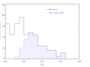
Figure 2: Distribution of measured amplitude of variability for all objects (solid line) and for the sources where flux variability was detected with a confidence level $\geq 3\sigma$ (filled histogram).

4.1 Amplitude of flux variability

The method we have used to calculate the amplitude of flux variability (noise-subtracted) in our light curves is fully described in Almaini et al. (Almaini00 (2000)). This method is the most appropriate in the regime of Gaussian statistics, an assumption that, as we said before, is satisfied by our data. In addition, this method is appropriate for light curves with points having significantly different measurement errors.

The method assumes that the measured dispersion in the light curves has two different contributions:

$$\sigma_{{\rm total}}^{2}=\sigma_{{\rm noise}}^{2}+\sigma_{Q}^{2}$$ (2)

The first contribution, $\sigma_{noise}$, is the statistical error in the data points and the second, $\sigma_{Q}$, the true fluctuation in the source flux. We are interested in the second quantity, $\sigma_{Q}$, as it measures the intrinsic variability in flux of the objects. In order to calculate $\sigma_{Q}$, a maximum likelihood method is used.

Table 3: Measured values of 0.2-12 keV flux variability amplitudes in Lockman Hole sources.

Sample	${\rm\langle\sigma_{{\rm intr}}\rangle_{all}}$	${\rm\langle\sigma_{{\rm intr}}\rangle_{all}^{w}}$	${\rm\langle\sigma_{{\rm intr}}\rangle_{var}}$	${\rm\langle\sigma_{{\rm intr}}\rangle_{var}^{w}}$	${\rm\sigma_{{\rm intr}}}$
(1)	(2)	(3)	(4)	(5)	(6)
All	0.22$\pm$0.01	$0.15\pm 0.01$	0.34$\pm$0.01	0.28$\pm$0.01	$\leq$0.36
type-1 AGN	0.27$\pm$0.02	$0.18\pm 0.02$	0.34$\pm$0.02	0.27$\pm$0.02	$0.27_{-0.08}^{+0.47}$
type-2 AGN	0.21$\pm$0.03	$0.15\pm 0.02$	0.34$\pm$0.04	0.28$\pm$0.02	$\leq 0.35$
Unidentified	0.19$\pm$0.02	$0.11\pm 0.02$	0.35$\pm$0.03	0.30$\pm$0.02	$\leq 0.33$

• Columns are as follows: (1) group of sources; (2) arithmetic means and corresponding 1$\sigma$ errors of the measured variability amplitudes for different types of sources; (3) weighted means and corresponding 1$\sigma$ errors of the measured variability amplitudes for different types of sources; (4) and (5) arithmetic and weighted means of the measured variability amplitudes considering only objects with detected variability from the $\chi^{2}$ test; (6) mode and 1$\sigma$ confidence intervals from the average ${\rm P(\sigma_{{\rm intr}})}$ distributions. For the cases where the integral of the ${\rm P(\sigma_{{\rm intr}})}$ distribution to the left reached zero 68% confidence upper limits are given.

For each object, a probability distribution for $\sigma_{Q}$ is obtained. The maximum of this function gives the most probable value of $\sigma_{Q}$ for the given set of data points, while the uncertainty in $\sigma_{Q}$ is obtained by integrating the function from the maximum value to both sides until the desired probability is encompassed. We have calculated 1$\sigma$ errors for the measured variability amplitudes. In the cases where the lower error bound of the integrals reached zero we calculated 1$\sigma$ upper limits for $\sigma_{Q}$.

To allow comparison of variability amplitudes for sources with different mean count rates we have calculated the value of the normalised excess variance, $\sigma_{{\rm intr}}$, for each source,

$$\sigma_{{\rm intr}}={\sigma_{Q}\over\langle{\it CR}\rangle}$$ (3)

where $\langle{\it CR}\rangle$ is the unweighted mean 0.2-12 keV count rate of that source. This parameter gives the fraction of the total flux that is variable, and therefore can be used to compare amplitudes of flux variability for sources with different fluxes. Fig. 1 shows typical probability distributions of $\sigma_{{\rm intr}}$ of sources without detected (top) and detected (bottom) variability.

The distribution of $\sigma_{{\rm intr}}$ values obtained from the light curves of our sources is shown in Fig. 2 for the whole sample of objects (solid line) and for objects where flux variability was detected in terms of the $\chi^{2}$ test with a confidence $\geq$3$\sigma$ (filled histogram).

We see that our variable sources have a broad range of values of the measured excess variance from $\sim$10% to $\sim$65%, with the maximum of the distribution (for objects with detected variability) being at a value of $\sim$30%. Values of the excess variance above $\sim$50-60% are not common in our sources.

We expect the efficiency of detection of variability to be a strong function of the quality of the light curves, but also of the amplitude of variability. Therefore the fraction of sources with detected variability from the $\chi^{2}$ test should decrease for lower variability amplitudes. This effect is evident from Fig. 2, where we see that, for variability amplitudes lower than 20%, the values of the amplitude formally obtained are very rarely significant at 3$\sigma$.

Therefore our distribution of observed flux variability amplitudes for variable objects should not be interpreted as a true distribution of variability amplitudes in our sample of sources. Indeed we might be missing sources with low variability amplitudes or faint sources with strong variability due to the large statistical errors in the data. We will return to this point in Sec. 4.3.

4.2 Mean variability amplitude

  

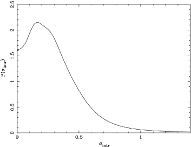
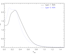
Figure 3: Mean probability density functions of the excess variance, $P(\sigma_{{\rm intr}})$, for all objects (top) and for type-1 and type-2 AGN (bottom). The distributions were obtained from the mean of the individual probability distributions of $\sigma_{{\rm intr}}$.

Mean values of $\sigma_{{\rm intr}}$ for the whole sample of sources and for type-1 and type-2 AGN and unidentified subsamples are listed in Table 3. We show values obtained using both the arithmetic and weighted mean for comparison. We see that average values from the weighted mean are significantly lower that those obtained with the arithmetic mean in all cases. This is because, as we want to study the variability properties of our sample, we included in the calculations all measured values of ${\rm\sigma_{intr}}$ independently on whether we detected or not significant variability in the light curves. Because of that, we have a number of sources with measured $\sigma_{{\rm intr}}$ values of zero but with errors of the same order as the ones for $\sigma_{{\rm intr}}$$>$0. These values shift the weighted means to lower values.

We see in Table 3 that the mean values for the amplitude of flux variability for type-1 and type-2 AGN do not differ significantly.

Table 4: Summary of detection of X-ray variability in Lockman Hole sources

$XMM$	ROSAT	R.A.	Dec	Class	redshift	Model	Flux var	Spec var	$\sigma_{{\rm intr}}$
(1)	(2)	(3)	(4)	(5)	(6)	(7)	(8)	(9)	(10)
607	-	10 53 01.86	+57 15 00.69	–	-	SPL	$>$99.99	$>$99.99	$\leq$ 0.65
599	54A	10 53 07.46	+57 15 05.84	type-1	2.416	SPL	$>$99.99	45.9	$0.25_{0.11}^{0.35}$
400	13A	10 52 13.29	+57 32 25.58	type-1	1.873	SPL	$>$99.99	81.5	$0.20_{0.14}^{0.25}$
63	-	10 52 36.49	+57 16 04.07	–	-	APL	5.5	93.4	$\leq$ 0.11
5	52A	10 52 43.30	+57 15 45.95	type-1	2.144	SPL	$>$99.99	25.1	$0.17_{0.10}^{0.22}$
6	504(51D)	10 51 14.30	+57 16 16.88	type-2	0.528	SPL	60.9	66.7	$\leq$ 0.26
16	-	10 51 46.64	+57 17 16.02	–	-	APL	44.0	45.9	$\leq$ 0.31
21	48B	10 50 45.67	+57 17 32.60	type-2	0.498	SPL	-1.0	-1.0	$-_{-}^{-}$
26	-	10 52 32.99	+57 17 50.96	–	-	SPL	12.1	1.3	$\leq$ 0.20
31	-	10 52 00.34	+57 18 08.24	–	-	CAPL	$>$99.99	99.8	$\leq$ 0.77
41	46A	10 51 19.14	+57 18 34.09	type-1	1.640	APL	-	-	$-_{-}^{-}$
39	45Z	10 53 19.09	+57 18 53.58	type-2	0.711	SPL	$>$99.99	51.9	$0.22_{0.11}^{0.31}$
53	43A	10 51 04.39	+57 19 23.90	type-1	1.750	APL	19.3	61.6	$\leq$ 0.10
65	-	10 52 55.46	+57 19 52.80	–	-	APL	87.6	85.3	$0.18_{0.03}^{0.32}$
74	905A	10 52 51.13	+57 20 15.70	–	-	SPL	83.9	69.5	$\leq$ 0.28
72	84Z	10 52 16.94	+57 20 19.71	type-2	2.710	APL	$>$99.99	55.0	$0.29_{0.20}^{0.36}$
85	38A	10 53 29.50	+57 21 06.22	type-1	1.145	SPL	$>$99.99	70.7	$0.39_{0.27}^{0.48}$
86	-	10 53 09.68	+57 20 59.58	type-1	3.420	SPL	8.3	54.1	$\leq$ 0.10
88	39B	10 52 09.37	+57 21 05.43	type-1	3.279	SPL	$>$99.99	74.4	$0.46_{0.23}^{0.59}$
90	37A	10 52 48.09	+57 21 17.43	type-1	0.467	SPL+SE	$>$99.99	$>$99.99	$0.64_{0.40}^{0.81}$
96	814(37G)	10 52 44.87	+57 21 24.84	type-1	2.832	SPL	$>$99.99	43.3	$0.19_{0.12}^{0.25}$
107	-	10 52 19.49	+57 22 15.26	type-2	0.075	APL	89.6	84.9	$\leq$ 0.20
120	-	10 52 25.17	+57 23 07.02	–	-	SPL	$>$99.99	69.9	$\leq$ 0.41
108	-	10 50 50.91	+57 22 15.65	–	-	2SPL	88.7	49.0	$\leq$ 0.16
900	-	10 54 59.43	+57 22 18.84	–	-	APL	35.3	34.6	$\leq$ 0.17
121	434B	10 52 58.08	+57 22 51.95	type-2	0.772	APL	98.2	29.4	$0.16_{0.07}^{0.24}$
135	513(34O)	10 52 54.39	+57 23 43.89	type-1	0.761	SPL	$>$99.99	63.2	$0.26_{0.18}^{0.32}$
124	634A	10 53 11.72	+57 23 09.07	type-1	1.544	SPL	90.0	64.0	$0.12_{0.03}^{0.19}$
125	607(36Z)	10 52 19.90	+57 23 07.92	–	-	SPL	$>$99.99	28.1	$\leq$ 0.47
142	-	10 52 03.74	+57 23 39.62	–	-	SPL	88.5	97.7	$0.16_{0.05}^{0.27}$
133	35A	10 50 38.77	+57 23 39.67	type-1	1.439	SPL	-1.0	-1.0	$-_{-}^{-}$
148	32A	10 52 39.66	+57 24 32.83	type-1	1.113	SPL+SE	$>$99.99	65.7	$0.30_{0.22}^{0.37}$
166	-	10 52 31.98	+57 24 30.82	–	-	APL	78.2	$>$99.99	$0.10_{0.01}^{0.20}$
156	-	10 51 54.59	+57 24 09.28	type-2	2.365	APL	99.2	95.6	$\leq$ 0.30
163	33A	10 51 59.88	+57 24 26.31	type-1	0.974	APL	$>$99.99	89.7	$0.33_{0.21}^{0.44}$
168	31A	10 53 31.72	+57 24 56.19	type-1	1.956	SPL	$>$99.99	68.6	$0.53_{0.38}^{0.66}$
172	-	10 53 15.71	+57 24 50.84	type-2	1.17	APL	60.2	$>$99.99	$\leq$ 0.22
183	82A	10 53 12.27	+57 25 08.28	type-1	0.96	SPL	$>$99.99	74.4	$0.28_{0.18}^{0.36}$
176	30A	10 52 57.25	+57 25 08.77	type-1	1.527	SPL	$>$99.99	59.1	$0.32_{0.22}^{0.41}$
179	-	10 52 31.64	+57 25 03.93	–	-	CAPL	85.5	$>$99.99	$0.15_{0.01}^{0.31}$
174	-	10 51 20.63	+57 24 58.24	–	-	SPL	$>$99.99	53.3	$\leq$ 0.64
186	-	10 51 49.93	+57 25 25.13	type-2	0.676	APL	$>$99.99	41.0	$0.34_{0.18}^{0.46}$
171	28B	10 54 21.22	+57 25 45.40	type-2	0.205	APL	$>$99.99	62.0	$\leq$ 0.17
200	-	10 53 46.81	+57 26 07.77	–	-	APL	90.6	45.8	$0.14_{0.03}^{0.25}$
187	-	10 50 47.96	+57 25 22.71	–	-	SPL	$>$99.99	81.6	$\leq$ 0.49
191	29A	10 53 35.03	+57 25 44.13	type-1	0.784	SPL	$>$99.99	90.6	$0.50_{0.31}^{0.64}$
199	-	10 52 25.28	+57 25 51.27	–	-	APL	99.9	$>$99.99	$0.16_{0.06}^{0.25}$
217	-	10 51 11.60	+57 26 36.67	–	-	APL	99.3	60.0	$0.14_{0.06}^{0.23}$
214	-	10 53 15.09	+57 26 30.65	–	-	APL	98.8	97.9	$0.18_{0.06}^{0.30}$
222	-	10 53 51.67	+57 27 03.64	type-2	0.917	APL	$>$99.99	$>$99.99	$0.25_{0.16}^{0.33}$
2020	27A	10 53 50.19	+57 27 11.61	type-1	1.720	SPL	$>$99.99	53.6	$0.43_{0.30}^{0.53}$
226	-	10 51 20.49	+57 27 03.47	–	-	SPL	99.9	98.8	$0.21_{0.09}^{0.30}$
243	-	10 51 28.14	+57 27 41.55	–	-	CAPL	$>$99.99	$>$99.99	$0.25_{0.14}^{0.33}$
254	486A	10 52 43.37	+57 28 01.49	type-2	1.210	APL	$>$99.99	13.6	$0.30_{0.16}^{0.42}$
261	80A	10 51 44.63	+57 28 08.89	type-1	3.409	SPL	$>$99.99	95.9	$0.22_{0.14}^{0.30}$
259	-	10 53 05.60	+57 28 12.50	type-2	0.792	APL+SE	71.2	$>$99.99	$\leq$ 0.10
270	120A	10 53 09.28	+57 28 22.65	type-1	1.568	SPL+SE	$>$99.99	97.7	$0.15_{0.10}^{0.20}$
267	428E	10 53 24.54	+57 28 20.65	type-1	1.518	APL	$>$99.99	32.1	$0.28_{0.20}^{0.35}$
287	821A	10 53 22.04	+57 28 52.76	type-1	2.300	SPL	$>$99.99	99.8	$0.25_{0.14}^{0.33}$
268	-	10 53 48.09	+57 28 17.75	–	-	APL	96.0	99.1	$0.17_{0.06}^{0.27}$
277	25A	10 53 44.85	+57 28 42.24	type-1	1.816	SPL	$>$99.99	77.1	$0.51_{0.38}^{0.62}$
272	26A	10 50 19.40	+57 28 13.99	type-2	0.616	APL	80.9	33.0	$\leq$ 0.21
290	901A	10 52 52.74	+57 29 00.81	type-2	0.204	APL+SE	98.3	$>$99.99	$0.13_{0.03}^{0.22}$
369	-	10 51 06.50	+57 15 31.92	–	-	SPL	96.9	15.7	$\leq$ 0.31
300	426A	10 53 03.64	+57 29 25.56	type-1	0.788	CAPL	$>$99.99	99.0	$0.35_{0.21}^{0.45}$
306	-	10 52 06.84	+57 29 25.43	type-2	0.708	APL	98.3	77.0	$0.19_{0.06}^{0.30}$
321	23A	10 52 24.74	+57 30 11.40	type-1	1.009	SPL	$>$99.99	$>$99.99	$0.20_{0.07}^{0.29}$
326	117Q	10 53 48.80	+57 30 36.09	type-2	0.78	APL	$>$99.99	96.7	$0.37_{0.26}^{0.46}$
350	-	10 52 41.65	+57 30 39.97	–	-	SPL	43.1	94.1	$\leq$ 0.12
332	77A	10 52 59.16	+57 30 31.81	type-1	1.676	SPL	$>$99.99	98.4	$0.31_{0.23}^{0.38}$
411	53A	10 52 06.02	+57 15 26.41	type-2	0.245	CAPL	95.4	4.8	$\leq$ 0.19
2024	-	10 54 10.68	+57 30 56.73	–	-	SPL	98.9	99.6	$0.15_{0.07}^{0.23}$
343	-	10 50 41.22	+57 30 23.31	–	-	SPL	70.5	96.3	$\leq$ 0.32
342	16A	10 53 39.62	+57 31 04.89	type-1	0.586	SPL+SE	$>$99.99	34.7	$0.44_{0.31}^{0.55}$
351	-	10 51 46.39	+57 30 38.14	–	-	SPL	99.1	37.4	$0.19_{0.08}^{0.29}$
353	19B	10 51 37.27	+57 30 44.43	type-1	0.894	SPL	94.7	77.0	$0.12_{0.03}^{0.20}$
354	75A	10 51 25.25	+57 30 52.33	type-1	3.409	SPL	$>$99.99	80.9	$0.35_{0.24}^{0.44}$
358	17A	10 51 03.86	+57 30 56.65	type-1	2.742	SPL	49.8	99.3	$\leq$ 0.08
355	-	10 52 37.33	+57 31 06.67	type-2	0.708	APL	$>$99.99	18.4	$\leq$ 0.86
385	14Z	10 52 42.37	+57 32 00.64	type-2	1.380	APL	99.6	$>$99.99	$0.14_{0.07}^{0.19}$
364	18Z	10 52 28.36	+57 31 06.57	type-1	0.931	SPL	93.2	99.7	$0.11_{0.02}^{0.19}$
901	-	10 50 05.55	+57 31 09.01	–	-	SPL	86.3	35.1	$\leq$ 0.21
902	73C	10 50 09.12	+57 31 46.29	type-1	1.561	SPL	92.4	99.5	$\leq$ 0.35
377	-	10 52 52.11	+57 31 38.02	–	-	APL	$>$99.99	62.0	$0.43_{0.16}^{0.62}$
384	-	10 53 21.63	+57 31 49.44	–	-	APL	64.0	71.6	$\leq$ 0.15
387	15A	10 52 59.78	+57 31 56.69	type-1	1.447	SPL	$>$99.99	86.2	$0.34_{0.22}^{0.44}$
394	-	10 52 51.40	+57 32 02.03	type-2	0.664	APL	98.8	21.0	$0.24_{0.10}^{0.37}$
406	828A	10 53 57.16	+57 32 44.00	type-1	1.282	SPL	$>$99.99	28.9	$0.38_{0.24}^{0.49}$
419	-	10 54 00.46	+57 33 22.19	–	-	APL	97.3	54.2	$0.16_{0.06}^{0.27}$
407	12A	10 51 48.69	+57 32 50.07	type-2	0.990	CAPL	$>$99.99	$>$99.99	$0.30_{0.22}^{0.37}$
424	-	10 52 37.93	+57 33 22.65	type-2	0.707	APL+SE	$>$99.99	$>$99.99	$0.28_{0.15}^{0.39}$
427	-	10 52 27.88	+57 33 30.65	type-2	0.696	SPL	$>$99.99	$>$99.99	$\leq$ 0.89
430	11A	10 51 08.19	+57 33 47.06	type-1	1.540	APL	91.0	95.3	$\leq$ 0.11
458	-	10 51 06.22	+57 34 36.67	–	-	CAPL	$>$99.99	94.7	$\leq$ 0.34
442	805A	10 53 47.28	+57 33 50.41	type-1	2.586	SPL	95.7	52.1	$0.21_{0.05}^{0.36}$
443	-	10 52 36.89	+57 33 59.80	type-2	1.877	APL	69.7	99.1	$\leq$ 0.20
474	-	10 51 28.13	+57 35 04.20	–	–	SPL	90.8	99.9	$0.11_{0.02}^{0.20}$
451	-	10 52 07.87	+57 34 17.48	–	-	APL	67.4	97.0	$\leq$ 0.19
450	477A	10 53 05.98	+57 34 26.70	type-1	2.949	SPL	$>$99.99	$>$99.99	$0.19_{0.11}^{0.25}$
453	804A	10 53 12.24	+57 34 27.39	type-1	1.213	SPL	99.6	45.2	$0.17_{0.08}^{0.25}$
456	9A	10 51 54.30	+57 34 38.66	type-1	0.877	SPL	$>$99.99	90.0	$0.53_{0.38}^{0.66}$
491	-	10 51 41.91	+57 35 56.00	–	-	APL	91.3	87.9	$0.14_{0.02}^{0.26}$
469	-	10 54 07.21	+57 35 24.89	–	-	SPL	$>$99.99	38.8	$0.43_{0.29}^{0.53}$
475	6A	10 53 16.51	+57 35 52.23	type-1	1.204	SPL	$>$99.99	5.4	$0.45_{0.35}^{0.55}$
476	827B	10 53 03.43	+57 35 30.80	type-2	0.607	SPL	$>$99.99	67.9	$0.27_{0.15}^{0.37}$
505	104A	10 52 41.54	+57 36 52.85	type-2	0.137	CAPL	$>$99.99	99.6	$0.47_{0.32}^{0.59}$
504	-	10 54 26.22	+57 36 49.05	–	-	APL+SE	$>$99.99	66.0	$\leq$ 0.54
511	-	10 53 38.50	+57 36 55.47	type-2	0.704	APL+SE	7.0	$>$99.99	$\leq$ 0.14
518	-	10 53 36.33	+57 37 32.14	–	–	APL	67.4	60.8	$\leq$ 0.20
523	-	10 51 29.98	+57 37 40.71	–	-	SPL	$>$99.99	99.8	$0.49_{0.30}^{0.62}$
529	-	10 51 37.30	+57 37 59.11	–	-	CAPL	99.0	71.2	$0.13_{0.04}^{0.21}$
532	801A	10 52 45.36	+57 37 48.69	type-1	1.677	SPL	76.9	38.7	$\leq$ 0.23
527	5A	10 53 02.34	+57 37 58.62	type-1	1.881	SPL	92.6	4.3	$0.07_{0.02}^{0.12}$
537	-	10 50 50.04	+57 38 21.79	–	-	SPL	$>$99.99	84.2	$\leq$ 1.26
548	832A	10 52 07.53	+57 38 41.40	type-1	2.730	SPL	95.1	$>$99.99	$0.20_{0.04}^{0.33}$
557	-	10 52 07.75	+57 39 07.49	–	-	APL	1.1	4.5	$\leq$ 0.12
553	2A	10 52 30.06	+57 39 16.81	type-1	1.437	APL	$>$99.99	99.9	$0.32_{0.24}^{0.40}$
555	-	10 51 52.07	+57 39 09.41	–	-	SPL	98.8	17.9	$0.18_{0.02}^{0.29}$
594	-	10 52 48.40	+57 41 29.14	–	-	SPL	99.9	80.0	$\leq$ 0.58
2045	-	10 52 04.47	+57 41 15.65	–	-	SPL	$>$99.99	99.9	$\leq$ 0.59
584	-	10 52 06.28	+57 41 25.53	–	-	SPL	$>$99.99	97.7	$0.28_{0.13}^{0.39}$
591	-	10 52 23.17	+57 41 24.62	–	–	SPL	88.6	89.5	$0.11_{0.02}^{0.20}$
601	-	10 51 15.91	+57 42 08.59	–	-	SPL	76.9	81.3	$\leq$ 0.21

Table 4: Continued

Columns are as follows: (1) Source X-ray identification number; (2) ROSAT identification number; (3) Right ascension (J2000); (4) Declination (J2000); (5) object class based on optical spectroscopy; (6) redshift; (7) Best fit model of the co-added spectrum of each individual source (from Mateos et al.(2005b) 2005b ); (8) Significance of 0.2-12 keV flux variability (in %); (9) Significance of spectral variability (in %); (10) Variability amplitude. Errors correspond to the 1$\sigma$ confidence interval. For the objects where the lower error bar reached zero 68% upper limits are given.

We have calculated the mean probability distribution of the excess variance, $P(\sigma_{{\rm intr}})$, for our sample of sources as the unweighted average of the probability distributions of $\sigma_{{\rm intr}}$ obtained from each light curve. As we mentioned before, because we want to describe the X-ray flux variability properties for the sample as a whole, we have included in the calculation the probability distributions of $\sigma_{intr}$ for both variable and non variable sources. These mean probability distributions are shown in Fig. 3 for all sources (top) and for the two AGN samples (bottom). The most probable values (modes) and the corresponding 1$\sigma$ uncertainties obtained from these distributions are listed in column 6 of Table 3. The mode for the whole sample of sources is $\sigma_{{\rm intr}}$$\sim$0.15 (68% upper limit =0.36), consistent with the value obtained from the arithmetic mean of the values for each source, as expected.

We see that the average probability distributions of $\sigma_{{\rm intr}}$ for type-1 and type-2 AGN do not differ significantly, although the most probable value of $\sigma_{{\rm intr}}$ is marginally lower for type-2 AGN than for type-1 AGN.

The flux variability properties for all our sources (significance of detection and amplitude of variability) are listed in Table LABEL:summary_var_det. The first and second columns list the XMM-Newton and ROSAT identification number of the sources. Columns 3 and 4 show the coordinates of the sources while columns 5 and 6 list the optical class and spectroscopic redshift. Column 7 lists the best fit model from the spectral analysis of the co-added spectra of our objects (from Mateos et al. 2005b ). The next three columns list the results of the detection of flux and spectral variability.

4.3 Probability distribution of the excess variance

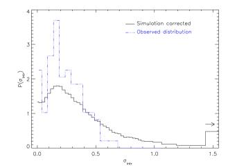
Figure 4: Distribution of intrinsic amplitude of flux variability, $P(\sigma_{{\rm intr}})$, obtained from our simulations (solid line). Note that in our simulations (see Appendix B) we referred to the measured amplitude of flux variability as $\sigma_{obs}$ or $S_{o}$ instead of $\sigma_{intr}$. The distribution of values obtained for our sample of sources (excluding objects with less than 5 points in their light curves, see Sec. 4.3) is shown for comparison (dashed line).

There are a number of factors that could be affecting the values and distribution of measured excess variances that we utilised to model the flux variability. The most clear example is the low quality in our light curves. We have made simulations in order to obtain the true probability distribution of excess variance for our sources, after accounting for all the selection effects in our sample of objects. The details on how the simulations were carried out are given in Appendix B. These simulations assume that the flux variability properties are not dependent on the source’s flux (or count rate), an assumption that is consistent with our analysis.

Our simulations have shown that the observed amplitude of variability depends strongly on the number of points in the light curves, in the sense that systematically lower amplitudes of variability are measured in objects with smaller number of points in the light curves. Therefore in this section we use only the 103 sources with at least 5 points in their light curves. The “corrected” probability distribution, $P(\sigma_{{\rm intr}})$, obtained using our simulations is shown in Fig. 4 (solid line). To witness the effects that go into this, we also have included the observed probability distribution of $\sigma_{{\rm intr}}$ values (dashed-line) for our sources, excluding objects with less than 5 points in their light curves (see Fig. 2).

We see that both distributions peak at similar values of $\sigma_{{\rm intr}}$$\sim$0.2 and therefore effects as the ones listed before, are not affecting significantly the mode of the distribution of amplitudes of flux variability. However the corrected distribution of intrinsic excess variances shows a long tail towards high values of $\sigma_{{\rm intr}}$ ($\geq$0.6), which we failed to detect in the real data. During our simulations work we found that for sources with light curves with the lowest number of bins, we always measured values of the variability amplitude significantly lower than the input value, no matter how large this value was (see Fig. 17). Hence, we can explain the scarcity of sources in which we have detected large ($\geq$0.6) variability amplitudes as being due to a small number of points in the light curve.

4.4 Dependence of flux variability with luminosity and redshift

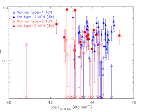
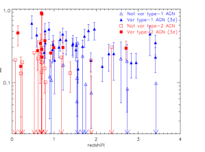
Figure 5: Dependence of the excess variance, $\sigma_{{\rm intr}}$, on the absorption corrected 2-10 keV luminosity (obtained from the best fit model of each object, left) and redshift (right) for our sample of AGN. Errors correspond to the 1$\sigma$ confidence interval.

It has been suggested that flux variability amplitude, when measured on a fixed temporal frequency, correlates inversely with X-ray luminosity (this has been confirmed on short time scales, $\sim$1 day) for nearby Seyfert 1 galaxies (Barr et al. Barr86 (1986); Lawrence et al. Lawrence93 (1993); Nandra et al. Nandra97 (1997)), in the sense that more luminous sources show lower variability amplitudes than less luminous sources. However there is significant scatter in this correlation on both short and long time scales, which has been attributed for example, to a dependence of the amplitude of variability on the spectral properties of the sources (Fiore et al. Fiore98 (1998); Green et al. Green93 (1993)). Furthermore, there are also indications that the strength of the correlation decreases towards longer time scales (Markowitz et al. Markowitz04 (2004)) and might be weaker for sources at higher redshifts (Almaini et al. Almaini00 (2000); Manners et al. Manners02 (2002)).

Table 5: Amplitudes of variability obtained from the mean probability distributions of $\sigma_{{\rm intr}}$ for type-1 AGN at different luminosities and redshifts.

Group	$\sigma_{{\rm intr}}$
(1)	(2)
type-1 AGN z$<$1.5	$0.32_{-0.23}^{+0.17}$
type-1 AGN z$>$1.5	$0.18_{-0.17}^{+0.17}$
type-1 AGN $L_{\rm(2-12\,keV)}>10^{44}$	$\leq$0.38
type-1 AGN $L_{\rm(2-12\,keV)}<10^{44}$	$0.29_{-0.20}^{+0.20}$

• Columns are as follows: (1) type-1 AGN group; (2) variability amplitude, $\sigma_{{\rm intr}}$, obtained from the mode of the mean probability distributions, $P(\sigma_{{\rm intr}})$, of each group of sources. Errors correspond to the 1$\sigma$ confidence interval. In the cases where the lower error bound of the integrals reached zero we calculated 90% upper limits for $\sigma_{intr}$.

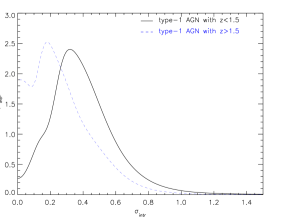
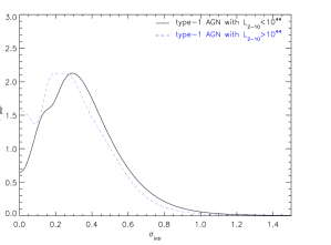
Figure 6: Left: Average probability distributions of $\sigma_{{\rm intr}}$ for sources with redshifts below 1.5 and above 1.5. Right: Average probability distributions of $\sigma_{{\rm intr}}$ for sources at 2-10 keV luminosities above and below $10^{44}\,{\rm erg\,s^{-1}}$. The probability distributions were obtained using all AGN, variable and non variable in terms of the $\chi^{2}$ test.

We have analysed whether there exists any dependence of the detected flux variability in our sources with their X-ray luminosity and redshift. Fig. 5 (left) shows the measured variability amplitudes for our AGN as a function of the 2-10 keV luminosity. We have used the absorption-corrected 2-10 keV luminosities obtained from the best fit of the co-added spectrum of each object. The values we used are reported in Table 8 of Mateos et al. (2005b ). In order to determine the significance of any correlation between the two quantities we used the version of the generalised Kendall’s tau test provided in the Astronomy Survival Analysis package (ASURV; Lavalley et al. Lavalley92 (1992)) which implements the methods described in Isobe et al. Isobe86 (1986) for the case of censored data. The results of the Kendall’s $\tau$ test including the probability that a correlation is present are $\tau=0.05\,(4\%)$ for $\sigma_{intr}$-${\rm L_{2-10keV}}$ and $\tau=2.25\,(97.7\%)$ for $\sigma_{intr}$-redshift. We have derived linear regression parameters using the ”estimate and maximise” (EM) and the Buckley-James regression methods also included in the ASURV package, however as both methods agreed within the errors, we only give the results from the EM test. We found the relations between $\sigma_{intr}$-${\rm L_{2-10keV}}$ and $\sigma_{intr}$-redshift to be

$$\sigma_{intr}=(-0.012\pm 0.044)\times\,\log({\rm L_{2-10\,keV}})+(1.054\pm 1.937)$$ (4)

and

$$\sigma_{intr}=(-0.062\pm 0.028)\times\,{\rm z}+(0.378\pm 0.053)$$ (5)

We see that we do not find any anticorrelation between excess variance and luminosity. However it is important to note that the known anticorrelation was found when using the same rest-frame frequency interval for all sources, while the light curves of our sources are not uniformly distributed in time and cover much longer time scales than the ones used in those works.

Figure 7: Observed spectral variability of three objects in our sample for which their co-added spectra were best fitted with a simple power law. Variation of the continuum shape ($\Gamma$) with time (errors correspond to the 90% confidence interval). Horizontal lines indicate the best fit continuum shape (dashed lines) and the corresponding 90% confidence intervals (solid lines) measured in the co-added spectra.

We have used the same observed energy band to study the variability properties of our sources, but because our sources span a broad range in redshifts we are sampling different rest-frame energies (harder energies for higher redshift sources). This could be a problem when comparing observed variability properties between sources, if there exists a dependence of variability properties with energy (stronger variability in the soft band compared to the hard band, has been observed in a number of Seyfert 1 galaxies). By plotting the excess variance versus redshift we should be able to see whether this effect is present in our data. This dependence of $\sigma_{{\rm intr}}$ with redshift is shown in Fig. 5 (right). The results from the generalised Kendall’s tau test (probability of detection of 97.7% ) and from the linear regression analysis (Eq.5) suggest that there is a weak correlation between $\sigma_{{\rm intr}}$ and the redshift.

To enhance any underlying correlation between the amplitude of variability and the X-ray luminosity or redshift, we have obtained average probability distributions for our sample of type-1 AGN (we cannot repeat the experiment for type-2 AGN as the sample size is too small) in bins of redshift and luminosity. In order to have enough objects per bin and enough data points we have used only two bins in redshift and luminosity (all bins having the same number of objects). The results are shown in Fig. 6 while the values of $\sigma_{{\rm intr}}$ obtained from these distributions (modes) are shown in Table 5. The variability amplitude appears to be independent of the 2-10 keV luminosity, confirming the above results. The same result holds for the dependence of variability amplitude with redshift as we see that there is some indication that the amplitude of flux variability is lower for higher redshift sources, although the effect is not very significant.

In addition, we do not find that the detection of flux variability changes with redshift. In summary, neither the fraction of sources with variability or its amplitude change with redshift in our sample.

5 Spectral variability

Comptonization models are most popular in explaining the X-ray emission in AGN (Haardt et al. Haardt97 (1997)). In these models the X-ray emission is produced by Compton up-scattering of optical/UV photons in a hot electron corona above the accretion disc. One of the predictions of these models is that, if the nuclear emission increases, the Compton cooling in the corona should increase too, and therefore the corona will become colder, and the X-ray spectrum becomes softer.

This flux-spectral behaviour is similar to the one observed in different states of BHXRB (McClintock et al. McClintock03 (2003)): in the low/hard state, most commonly observed in these objects, their X-ray fluxes are low and the 2-10 keV X-ray spectra are dominated by non thermal emission, best reproduced by a hard ($\Gamma$$\sim$1.5-2.1) power law, along with a weak or undetected thermal component (multi-temperature accretion disk component). In the high/soft state their fluxes are high and their 2-10 keV spectra are soft, dominated by the thermal component with a temperature $\sim$1 keV.

The accretion disk-static hot corona model of Haardt et al. (Haardt97 (1997)) predicts that, if the corona is dominated by electron-positron pairs, an intensity variability of a factor of 10 over the 2-10 keV rest-frame band will correspond to a change in the spectral slope of $\Delta\Gamma$$\sim$0.2. The relation between spectral shape and intensity is less clear for a corona not dominated by pairs, but qualitatively significant spectral variations could be obtained for small changes in the observed count rate in this case.

In order to provide more insight into the nature of the X-ray variability in our objects, we have studied which fraction of the sources in our sample show spectral variability and in these cases whether there exists some correlation between the observed flux and spectral variability.

Figure 8: Contour diagrams showing the observed spectral variability in type-1 and type-2 AGN. Contours correspond to 1$\sigma$, 2$\sigma$ and 3$\sigma$ confidence

5.1 Variability of the broad band X-ray colours

Because our sources are typically faint, we cannot use their spectra from each revolution, as the uncertainties in the measured spectral parameters will be in most cases too large. Instead, we have used a broad band X-ray colour or hardness ratio (HR), that allows us to search for changes in the broad band spectral shape of the sources. We calculated for each source a “colour” curve where each point is the X-ray hardness ratio from each observation which is obtained as

$${\it HR^{r}=(CR_{h}^{r}-CR_{s}^{r})/(CR_{h}^{r}+CR_{s}^{r})}$$ (6)

where ${\it CR_{s}^{r}}$ and ${\it CR_{h}^{r}}$ are corrected count rates (see Appendix A) in the 0.5-2 keV (soft) and 2-12 keV (hard) energy bands for revolution r respectively. We used these two energy band definitions to separate better the most important spectral components found in the co-added spectra of our objects. Changes in the intrinsic absorbing column density or in the properties of the soft excess emission component will affect mostly the soft count rate, while changes in the shape of the broadband continuum will affect both soft and hard band count rates.

In order to search for objects with spectral variability, we used the $\chi^{2}$ test (see Sec. 4) and a threshold in the significance of detection of 3$\sigma$. Results are summarised in columns 5 and 6 of Table 2. The fractions of sources with detected spectral variability have been corrected for the expected spurious detections at the selected confidence level as shown in Mateos et al. (2005a ) and Stevens et al. (Stevens05 (2005)). We have detected spectral variability above a confidence level of 3$\sigma$ in 24 out of the 120 objects with light curves with at least 2 points. Spectral variability was detected in 6 out of 45 type-1 AGN and 9 out of 27 type-2 AGN. Among sources still not identified we detected spectral variability in 9 out of 48 (but note again the possible identification bias). These results indicate that spectral variability is much less common than flux variability. This result also holds for both samples of type-1 and type-2 AGN. This is not an unexpected result, as we know that with a limited number of counts, spectral variability is more difficult to detect than flux variability. As we will see in Sec. 7 (see Fig. 11), for a spectral pivoting model, a change in spectral slope of $\Delta\Gamma$$\sim$0.2 corresponds to a change in the observed X-ray colour of $\Delta$HR$\sim$0.1 while $\Delta$HR$\sim$0.2 requires $\Delta\Gamma$$\sim$0.4-0.6. The typical dispersion in HR values observed in our sources with detected spectral variability is $\sim$0.1-0.2 while most of the measurement errors in HR in a single observation are of similar size. Therefore changes in the continuum shape $\Delta\Gamma$$\leq$0.3 will be detectable only in a small number of objects in our sample. We will come back to this point in more detail in Sec. 6 and Sec. 7.

Finally, we have not found evolution with redshift of the fraction of objects with detected spectral variability, indicating that the effect of sampling harder rest-frame energy bands at higher redshifts does not reduce the detection of spectral variability.

We have compared the fractions of type-1 and type-2 AGN with detected spectral variability using the method described in Mateos et al. (2005a ). We found that the significance of these fractions being different is 99%. This constitutes marginal evidence that spectral variability might be more common in type-2 AGN, although we should recall that we are dealing with a small number of sources. If true, this might be due to the contribution to the X-ray emission from scattered radiation being higher in type-2 AGN. This scattered component will not be variable, as it will be related to the very distant reflector. The detected X-ray emission in type-2 AGN is dominated by the hard X-ray component (i.e., in the nuclear emission transmitted through the absorbing material) while most of the non-variable soft X-ray emission will not be significantly absorbed. Therefore, changes in the intensity of the hard X-ray component alone would result in larger changes in the observed X-ray colour.

5.2 Variability of the X-ray emission components

In order to give more insight into the nature of the detected spectral variability in our objects, we grouped the XMM-Newton observations in four different periods of time corresponding to the XMM-Newton phases PV, AO1 and AO2a and AO2b (see second column in Table 1). As we have said before, most of the objects in our sample are too faint to search for spectral variability comparing the emission properties measured on the X-ray spectrum from each revolution. A significant fraction of the exposure time was achieved during the AO2 phase, so we separated the AO2 data into two contiguous groups and still obtained data with enough quality for this analysis. We built for each object a co-added spectrum using the data from each observational phase. This approach allowed us to conduct standard spectral fitting and study spectral variability directly on time scales of months and years. We were able to carry out this study in 109 out of 123 objects for which we had more than one spectrum available. In order to search for spectral variability, we fitted the spectra of each observation phase with the best fit model (see column 7 in Table. LABEL:summary_var_det) and best fit parameters obtained from the overall spectrum of each object (see Table 8 in Mateos et al. 2005b ).

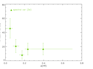
Figure 9: Top: Fraction of sources with detected flux variability as a function of the mean 0.2-12 keV count rate of the objects. Bottom: Fraction of sources with detected spectral variability as a function of the error in their mean X-ray colour.

We left free the normalisation of the continuum emission since we are only interested here in searching for spectral variability, and we have seen that flux variability is common. For sources with detected soft excess emission, we kept fixed the ratio of the soft excess to the power law normalisations that we found in the best fit of the co-added spectra. We then repeated the fits using the same spectral models, but allowing all fitting parameters to vary. We compared the $\chi^{2}$ of the two fits and searched for all cases where $\Delta\chi^{2}$=9 for one parameter and $\Delta\chi^{2}$=11.8 for two parameters, i.e. where we found a significant ($\geq$3$\sigma$) improvement in the quality of the fits varying the spectral shape. From this analysis we detected spectral variability in 8 (7%) sources (XMM-Newton identification numbers 400, 90, 148, 171, 191, 332, 342 and 469, see Table LABEL:summary_var_det), including 6 type-1 and 1 type-2 AGN. The fraction of objects with detected spectral variability increased to $\sim$17% if we used instead a confidence level of 2$\sigma$. We illustrate the observed spectral variability properties of the sources with detected spectral variability from this analysis in Fig. 7 for the 3 type-1 AGN best fitted with a power law (absorbed by the Galaxy). Fig. 8 shows some examples of contour diagrams of $\Gamma$-kT and $\Gamma-{\rm N_{H}}$ for variable AGN where absorption or soft excess were detected. We found that in all objects with detected spectral variability (including all AGN), this was associated mostly with changes in the shape of the broad band continuum ($\Delta\Gamma\sim$0.2-0.3 for all objects except source 90, where the observed maximum change in $\Gamma\sim$1 although with very large uncertainties). We did not see important changes in other spectral components such as the temperature of the soft excess component (when modelled with a black body) or the amount of intrinsic absorption. This is the case also for the one type-2 AGN in our sample with detected variability in its spectral fitting parameters.

Note that among the objects with detected spectral variability from this spectral fitting, we only detected spectral variability using the broad band X-ray colour in one source, 90 (see Table LABEL:summary_var_det). These results support the argument that the low fraction of objects with detected spectral variability could be due to the fact that typical changes in the continuum shape are of the order of $\Delta\Gamma$$\sim$0.2-0.3, which corresponds to $\Delta$HR$\sim$0.1, undetectable in most of the sources in our sample.

If this is the case, then the results shown in this section support the idea that the main driver (but not the only one, see later) for spectral variability on month-years scales in AGN might be changes in the mass accretion rate, resulting in changes in the underlying power law $\Gamma$. We will discuss this point in more detail in Sec. 7.

6 What is the true fraction of sources with X-ray variability?

In Fig. 9 (top) we show the fraction of objects in our sample with detected flux variability as a function of the mean 0.2-12 keV count rate. We see that it is a strong function of the mean count rate, and hence the number we obtained for the whole sample of objects ($\sim$50%) has to be taken as a lower limit. Indeed the plot suggests that the fraction of sources with flux variability might be 80% (the maximum fraction) or higher.

Figure 10: Correlation of flux and spectral variability properties for the 15 objects in our sample with detected flux and spectral variability with a confidence of more than 3$\sigma$. Errors correspond to the 1$\sigma$ confidence interval.

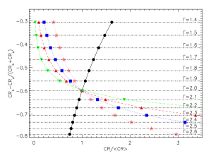
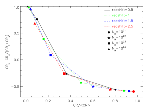
Figure 11: Left: Correlation of flux and spectral variability for a source at redshift of 1 associated with changes in the continuum shape alone for different rest-frame pivoting energies: 1 keV (circles), 10 keV (stars), 30 keV (squares), 100 keV (triangles) and 1000 keV (upside down triangles). Right: Correlation of flux and spectral variability associated with changes in the amount of intrinsic absorption alone at different redshifts: ${\rm N_{H}=10^{21},10^{22},10^{23},10^{24}cm^{-2}}$. For each absorption the size of the symbols represents the redshift, from redshift 0.5 (smallest symbol size) to redshift 2.5 (largest symbol size).

The result that the majority of our sources are variable in flux is in agreement with previous variability analyses, that found long time scale variability in AGN to be more common than short time scale variability (see e.g. Ciliegi et al. Ciliegi97 (1997); Grandi et al. Grandi92 (1992)). However not all sources in our sample are expected to be variable as some of the objects still not identified might either not be AGN, or be heavily obscured AGN.

Fig. 9 (bottom) shows the fraction of objects in our sample with detected spectral variability as a function of the mean error in the hardness ratio. We see that the detection of spectral variability varies with the quality of our data, although in this case a clear dependence is only evident for the first bin, which suggests that the fraction of sources in our sample with spectral variability could be $\sim$40% or higher.

Even if the fraction of sources with spectral variability is as high as $\sim$40%, this fraction is still significantly lower than the fraction of sources with flux variability. If spectral variability is less common than flux variability in our sample, then for many sources flux variability will not be accompanied by spectral variability.

                   

Figure 12: Flux variability properties for 4 of the sources in our sample spectroscopically classified as type-2 AGN but for which no absorption signatures were found in their co-added spectra (Mateos et al. 2005b ). Errors correspond to the 1$\sigma$ confidence interval. Horizontal lines indicate the mean CR over all revolutions (dashed lines) and the corresponding 1$\sigma$ confidence interval (solid lines).

                   

Figure 13: Spectral variability properties for the sources in our sample spectroscopically classified as type-2 AGN but for which no absorption signatures were found in their co-added X-ray spectra. Errors correspond to the 1$\sigma$ confidence interval. Horizontal lines indicate the mean HR over all revolutions (dashed lines) and the corresponding 1$\sigma$ confidence interval (solid lines).

7 On the long-term X-ray variability

The results of our variability analysis suggest that flux and spectral variability are not correlated for a significant fraction of the objects in our sample. Indeed 38 sources in our sample exhibit flux variability but not spectral variability, while 9 show spectral but not flux variability (see Table. LABEL:summary_var_det).

In addition, no evident correlation between flux and spectral variability was found for the 15 objects for which both were detected. The HR-CR plots for these objects are shown in Fig. 10. We see in Fig. 10 that significant changes in flux without evident changes in the X-ray colour are common in our objects. On the other hand important changes in the X-ray colour without significant flux variability have been detected in many of our sources.

The two-component spectral model and the spectral pivoting model have been frequently used to describe the flux and spectral variability properties in local Seyfert 1 galaxies. We have studied whether these phenomenological models can accommodate the variability properties of our objects, i.e. whether changes in the continuum shape alone can explain the observed spectral and flux variability detected in our objects. To do that we have assumed that the spectra of our sources can be well described with a power law (absorbed by the Galaxy). Then we have calculated the changes in HR and CR associated with variations of $\Gamma$ alone for different rest-frame pivoting energies and for a source at a redshift of 1. The results are shown in Fig. 11 (top) for pivoting energies of 1, 10, 30, 100 and 1000 keV.

We see that typical changes in $\Gamma$$\sim$0.2 correspond to small changes in the X-ray colour $\sim$0.1-0.2, which are undetectable in most of our sources. This could easily explain the lack of detection of spectral variability in a significant fraction of our sources. In addition, if the pivoting energy falls in the observed energy band (in the example of Fig. 11 this corresponds to pivoting energies of 1 keV and $\sim$10 keV), then spectral variability without significant changes in flux could be observed. However, in the cases where both flux and spectral variability are detected a correlation between the X-ray colour and flux should be evident, but as we see in Fig. 10 in the majority of the objects X-ray colour-flux trends are not observed. Furthermore, in order to explain with the spectral pivoting model the observed dispersion of X-ray colours changes in $\Gamma$ above 1 are required. If we take into account that in the majority of the Seyferts for which detailed variability studies are available, the detected pivoting energies are $\gg$10 keV (for example see Table 1 in Zdziarski et al. Zdziarski03 (2003)), then in most of our sources the pivoting energies are expected to be outside the observed energy band, and hence it is expected that changes in $\Gamma$$\gtrsim$1 will produce changes in flux much higher than those detected: these flux and spectral changes are not observed simultaneously in any of our sources. Finally, changes in $\Gamma$ of at least 1 are unlikely based on the predictions of thermal Comptonization models and the results shown in Sec. 5.2.

We conclude that it is unlikely that spectral pivoting alone can explain the observed trends in flux and spectral variability in our sources. The same result applies also to the two-component spectral model, as in this case as for the spectral pivoting model similar X-ray colour-flux trends are expected.

We have repeated our analysis to study the expected changes in X-ray colour and flux associated with changes in the amount of absorption alone. The results are shown in Fig. 11 (bottom), for different amounts of absorption and at different redshifts. Changes in absorption can be produced, for example, due to variations in the ionisation state of the absorber following changes in the ionising radiation, making the absorber more transparent. On the other hand, if the absorber is not homogeneous but clumpy (for example if it is made of clouds of gas moving around the central source), then variations in the column density along the line of sight will be expected due to clouds passing through the line of sight.

In this case both spectral and flux variability should be detected (see Fig. 11 bottom), but again, this is not the case for many objects in our sample. To produce changes in the X-ray colour that would be detected in our data, changes in absorption of ${\rm N_{H}\geq 5\times 10^{22}\,cm^{-2}}$ are required, especially if the sources are at redshifts greater than 1. Changes in ${\rm N_{H}}$ above this value could explain the observed amplitude of spectral variability seen in a fraction of our objects. However in this case, as we see in Fig. 11 (bottom), flux and spectral variability should be correlated: significant variations in absorption would be associated with significant changes in flux. It is very unlikely that variations in X-ray absorption alone can explain the variability properties of our sources.

Hence, from our analysis we conclude that

1. the lack of correlation between the observed flux and spectral variability properties of our objects indicates that the observed spectral variability is not triggered by changes in the X-ray luminosity of the sources.

2. the amplitude of the observed flux variability cannot be explained due to changes in the X-ray continuum shape or the amount of X-ray absorption alone.

3. The two-component spectral model and the spectral pivoting model do not describe properly the variability of our sources.

In order to explain both the flux and spectral variability properties of our sources, at least two parameters of the model must vary independently, such as, for example, the shape of the continuum or the amount of X-ray absorption, but also the continuum normalisation.

8 Variability properties of unabsorbed type-2 AGN

In Mateos et al. (2005b ) we showed that among the spectroscopically identified type-2 AGN in the sample of Lockman Hole sources selected, five did not show any signs of X-ray absorption in their co-added X-ray spectra (objects with identification number 6, 21, 39, 427 and 476). We have studied the flux and spectral variability properties of all these sources except source 21, for which only one data point was available. One of the hypotheses that could explain the disagreement between observed optical and X-ray properties in these sources is spectral variability: because the optical and X-ray observations were not obtained simultaneously, there might have been changes in the absorber during the time interval between the observations. Table LABEL:summary_var_det lists the flux and spectral variability properties of these sources, while their flux and X-ray colour curves are shown in Fig 12 and Fig. 13 respectively. We detected flux variability in 3 of the sources (39, 427 and 476); however spectral variability was only detected in one of the objects, source 427. Fig. 10 shows the flux vs spectral variability properties for source 427. We see that in four of the available observations flux variability was not seen, however changes in the HR are evident.

These sources were detected in a narrow redshift interval, from 0.5-0.7. In the previous section we have seen that at redshifts below 1, changes in the column density of the order of ${\rm N_{H}\sim 10^{21}\,cm^{-2}}$, affect the observed flux by $\sim$20%. However the corresponding change in the X-ray colour is only $\Delta$HR$\sim$0.05, and therefore impossible to detect in our data. If the changes in absorption were to be of the same magnitude as the typical absorption detected in our absorbed type-2 AGN (${\rm\sim 10^{22}\,cm^{-2}}$; see Figure 12 in Mateos et al. 2005b ) or larger, then changes in flux and in the X-ray colour will be significant ($\Delta$CR$\geq 30\%$ and $\Delta$HR$\geq 0.3$) and therefore we should have been able to detect them. Therefore, the lack of correlation between flux and spectral variability in these objects indicates that, for our unabsorbed type-2 AGN, variations in absorption of at least ${\rm N_{H}\geq 10^{22}\,cm^{-2}}$ are not observed in these objects. Moreover, the lack of detection of significant spectral variability in most of the sources makes unlikely that spectral variability alone can explain the observed mismatch of their optical-X-ray spectral properties as in these sources variations in the amount of absorption of at least ${\rm 10^{22}\,cm^{-2}}$ are expected.

Finally, the non detection of X-ray absorption in these objects cannot be explained by these sources being Compton-thick, because in this case, the X-ray emission should be dominated by scattered radiation (the varying nuclear component is largely undetected), and therefore we would not expect to detect flux or spectral variability in the sources on a time scale of $\leq$2 years.

9 Conclusions

We have carried out a detailed study of the X-ray spectral and flux variability properties of a sample of 123 sources detected with XMM-Newton in a deep observation in the Lockman Hole field. To study flux variability, we built for each object a light curve using the EPIC-pn 0.2-12 keV count rates of each individual observation. We obtained light curves for 120 out of 123 sources (the other three sources only had one bin in their light curves). We have searched for variability using the $\chi^{2}$ test. We detected flux variability with a confidence level of at least $3\sigma$ in 62 sources ($\sim$52%). However the efficiency of detection of variability depends on the amplitude of the variability. The observed strong decrease in the detection of variability in our sources at amplitudes $\leq$0.20 indicates that amplitudes of variability lower than this value cannot be detected in the majority of our sources. We also found that the fraction of sources with detected flux variability depends substantially on the quality of the data. The observed dependence suggests that the fraction of flux-variable sources in our sample could be 80% or higher, and therefore that the great majority of the X-ray source population (which at these fluxes is dominated by AGN) vary in flux on time scales of months to years, perhaps responding to changes in the accretion rate. Our results are consistent with the variability studies of Bauer et al. (Bauer03 (2003)) in the Chandra Deep Field-North and Paolillo et al. (Paolillo04 (2004)) in the Chandra Deep Field-South which found that the fraction of variable sources could be higher than $\sim$90%.

To measure the amplitude of the detected flux variability on each light curve above the statistical fluctuations of the data (excess variance), we used the maximum likelihood method described in detail in Almaini et al. (Almaini00 (2000)).

From this analysis we found the mean value of the relative excess variance to be $\sim$0.15 (68% upper limit being $\leq$0.36) for the whole sample of objects ($\sim 0.34\pm 0.01$ considering only sources with detected flux variability), although with a large dispersion in observed values (from $\sim$0.1 to $\sim$0.65). Values of excess variance larger than $\sim$50-60% were found not to be very common in our sources.

Similar values of the mean flux variability amplitude were found for the sub-samples of sources identified as type-1 and type-2 AGN, the fraction of variable sources being 68$\pm$11% for type-1 AGN and 48$\pm$15% for type-2 AGN.

We carried out extensive simulations in order to quantify the intrinsic true distribution of excess relative variance for our sources corrected for any selection biases. The most probable value of the true intrinsic amplitude of flux variability for our sample of objects is $\sim$0.2, as before correcting for selection biases. In addition, the simulations showed that the probability of detection of large variability amplitudes ($\geq$0.5) in our sample of sources is severely hampered by the poor quality of light curves.

Short time scale X-ray variability of Seyfert 1 galaxies indicate that the majority of these objects soften as they brighten. Our fainter and more distant sources do not generally follow this pattern. This should not be too surprising, as this effect is observed in light curves that sample a uniform time interval and on time scales much smaller than in our study, where the strength of the effect seems to be higher.

Because of the low signal-to-noise ratio of some of our data, we could not study spectral variability using the X-ray spectra of the sources from each observation, as the uncertainties on the fitted parameters would be too large. Hence, we used a broad band hardness ratio or X-ray colour to quantify the spectral shape of the emission of the objects on each observation. A $\chi^{2}$ test shows spectral (“colour”) variability with a confidence of more than 3$\sigma$ in 24 objects ($\sim$20$\pm$6% of the sample). However, we found the fraction of sources with detected spectral variability to increase with the quality of the data, hence this fraction could be as high as $\sim$40%. This fraction is still significantly lower than the fraction of sources with flux variability. However, we have shown that spectral variability is more difficult to detect than flux variability: a change in spectral slope of $\Delta\Gamma$$\sim$0.2-0.3 corresponds to a change in the observed X-ray Hardness Ratio of just $\Delta$HR$\sim$0.1. The typical dispersion in HR values in our sources with detected spectral variability is $\sim$0.1-0.2, i.e. of the same magnitude as most errors in the HR in a single observation. Therefore changes in the spectral index $\leq$0.3 will be only detectable in a small number of objects in our sample.

The fractions of AGN with detected spectral variability were found to be $\sim$14$\pm$8% for type-1 AGN and $\sim$34$\pm$14% for type-2 AGN with a significance of the fractions being different of $\sim$99%, i.e. 0.2-12 keV spectral variability on long time scales might be more common in type-2 AGN than in type-1 AGN. Although of only marginal significance, this result could be explained if part of the emission in type-2 AGN has a strong scattered radiation component. This component is expected to be much less variable and therefore changes in the intensity of the hard X-ray component alone would result in larger changes in the observed X-ray colour.

Our samples of type-1 and type-2 AGN cover a broad range in redshifts, especially the former. Therefore we have studied variability properties on significantly different rest-frame energy bands. We did not find a strong dependence on redshift of the observed fraction of sources with detected spectral and flux variability. On the other hand our analysis suggests that the amplitude of flux variability and the redshift might be correlated but the strength of the effect seems to be rather weak. Therefore we conclude that the overall flux and spectral X-ray variability properties of our AGN are very similar over the rest frame energy band from $\sim$0.2 keV to $\sim$54 keV.

We also grouped the spectra of our objects in four different observational phases, and compared the spectral fits to the grouped spectra. With this study we detected variations in spectral fit parameters in 8 objects, including 6 type-1 AGN and 1 type-2 AGN. A detailed analysis of their emission properties showed that the origin of the detected spectral variability is due to a change in the shape of their broad band continuum alone. In none of the sources we detected strong or significant changes in other spectral components, such as soft excess emission and/or X-ray absorption.

This result is confirmed by the spectral variability analysis of the 4 out of the 5 spectroscopically identified type-2 AGN for which we did not detect absorption in their co-added spectra. Flux variability was detected in 3 of the objects while only for one of them we detected spectral variability. The lack of detection of significant spectral variability in 3 out of 4 of the sources makes unlikely that variations in the absorber can explain the mismatch between their optical and X-ray spectral properties. In addition, we have shown that, if the change in absorption is of the same magnitude as the typical absorption detected in absorbed type-2 AGN, ${\rm N_{H}\sim 10^{22}\,cm^{-2}}$, then, changes in flux and in the X-ray colour will be significant ($\Delta$CR$\geq 30\%$ and $\Delta$HR$\geq 0.3$) and therefore we should have detected them. Therefore, the lack of correlation between flux and spectral variations in unabsorbed type-2 AGN indicates that, this is an intrinsic property and not just bad luck in non-simultaneous optical and X-ray observations. Finally, a Compton-thick origin for these sources is also very unlikely, as they are seen (3 out of 4) to vary in flux.

X-ray spectral variability in AGN on long time scales appears less common than flux variability. The same result seems to hold for both samples of type-1 and type-2 AGN. Therefore, flux and spectral variability might not be correlated in a significant fraction of our sources. Indeed in 38 objects we detected flux variability but not spectral variability, while spectral variability but not flux variability was detected in 9 objects. A correlation analysis of the flux-spectral variability properties on the 15 objects were both spectral and flux variability were detected only showed no obvious links.

Due to the apparent lack of correlation of flux and spectral variability, the two-component spectral model and the spectral pivoting model frequently used to explain the X-ray variability properties in local Seyfert 1 galaxies, cannot accommodate the variability properties of our sources, as both require flux and spectral variability to be correlated. For a source with a varying spectral index we have seen that in order to explain the detected amplitudes of flux variability a $\Delta{\it HR}\geq 0.3$ is required (which corresponds to $\Delta\Gamma\sim 0.6-1.2$). However such variability of HR is not observed. Furthermore, the amplitude of the observed flux variability cannot be explained due to changes in the X-ray continuum shape alone. This is confirmed by the fact that even in the objects with both spectral and flux variability detected, significant changes in HR are seen for almost constant values of the CR. Because of the apparent lack of correlation between flux and spectral variability, it is very unlikely that variations in X-ray absorption alone can explain the variability properties of our sources. Changes in absorption can be produced, but then both spectral and flux variability should be detected,and they are not. Therefore, the lack of correlation between the observed flux and spectral variability properties of our objects indicates that the observed spectral variability does not simply reflect changes in the X-ray luminosity of the sources. Furthermore, our variability study supports the idea that the driver for spectral variability on month-years scales in our AGN cannot be simply a change in the mass accretion rate. Clearly, more complex models are called for.

Appendix A Correction of count rates for calibration drifts

Figure 14: Corrections of the count rates for each revolution from systematic variations during the life time of the mission and from variations from using different blocking filters for the observations. From top to bottom corrections for the 0.2-12, 0.5-2 and 2-12 keV count rates. Errors correspond to the 1$\sigma$ confidence interval.

The XMM-Newton observations in the Lockman Hole span a broad range of the mission lifetime, and therefore, changes might be expected in the calibration of the data. Particularly in the instrumental spectral response and systematic variations in the background modelling with time. That could introduce systematic differences in the measured count rates of the same source between observations. In addition, pn observations were obtained with different blocking filters. A change in the blocking filter affects more the soft X-rays and therefore the measured 0.2-12 and 0.5-2 keV count rates.

In order to remove from the light curves the effects listed above, we have calculated for each revolution r the average deviation of the measured count rates in that revolution from their mean flux over all revolutions, for the subset of sources detected in that revolution. If there are no variations in the calibration, we would expect this value to be very close to unity, since variability is not expected to be correlated with time for different sources. We have called this value $\Omega^{r}$ and it is defined as,

$$\Omega^{r}={1\over N(r)}{\sum_{i=1}^{N(r)}{c_{i}^{r}\over\langle c_{i}\rangle}}$$ (7)

The sum is over the number of sources detected on each revolution r (N(r)), $c_{i}^{r}$ is the count rate of source i in revolution r and $\langle c_{i}\rangle$ is the mean unweighted count rate of the source over all revolutions where it was detected. We found that the errors in the count rates were dominated by the quality of the observations (the errors in the background modelling and fitting of the source parameters in the SAS source detection task emldetect), and do not depend strongly on the values of the count rates themselves, in the sense that sources with larger count rates do not tend to have smaller errors. Because of this, the use of the weighted mean is not necessary in this case, and therefore we used the unweighted mean to calculate the average flux of each source and the mean dispersion of the count rates of the sources from their mean values for each revolution. However our mean values could be significantly affected by outliers due to flux variability of the sources. In order to avoid this, we applied a sigma-clipping (3$\sigma$) before calculating average values.

The 1$\sigma$ errors in $\Omega^{r}$ will be $\sigma(\Omega^{r})/\sqrt{n(r)}$ where $n(r)$ is the number of points in revolution r after sigma-clipping i.e. $N(r)\rightarrow n(r)$, and $\sigma(\Omega^{r})$ is

$$[\sigma(\Omega^{r})]^{2}={1\over n(r)-1}{\sum_{i=1}^{n(r)}\left({c_{i}^{r}\over\langle c_{i}\rangle}-\Omega^{r}\right)}^{2}$$ (8)

We calculated values of $\Omega^{r}$ for the measured 0.2-12 keV count rates which we used to study flux variability, and for 0.5-2 keV and 2-12 keV count rates, which we used to carry out the study of spectral variability. The values of $\Omega^{r}$ and their corresponding 1$\sigma$ errors for each revolution and energy band are shown in Fig. 14.

The corrected count rates and their corresponding 1$\sigma$ errors for each revolution were obtained as

$$(c_{i}^{r})^{corr}={c_{i}^{r}\over\Omega^{r}}$$ (9)

$$\Delta(c_{i}^{r})^{corr}=((c_{i}^{r})^{corr})^{2}\times\sqrt{\left({\Delta c_{i}^{r}\over c_{i}^{r}}\right)^{2}+\left({\Delta\Omega^{r}\over\Omega^{r}}\right)^{2}}$$ (10)

It is evident from Fig. 14 that all the values are very close to unity, which means that we did not find calibration drifts between revolutions in any of the three energy bands, and therefore these corrections are very small in all cases.

Appendix B Simulations of variability in Lockman Hole sources

Figure 15: Distribution of 0.2-12 keV count rates (corrected for calibration uncertainties) in our sample of sources for which we studied flux variability.

In Sec. 4.1 we showed the distribution of variability amplitude that we found in our sample of objects. However measured values might differ from intrinsic values due to a number of effects, such as not enough quality in the light curves. In order to take into account all possible effects, we carried out simulations to calculate the distribution of intrinsic variability amplitude in our sample of objects after correcting for these effects.

In order to simplify the notation we will refer to the intrinsic amplitude of flux variability, $\sigma_{intr}^{i}$, as $S_{i}$, while ${\it S_{o}}$ will be used to refer to the corresponding measured amplitude, $\sigma_{intr}^{o}$. We defined a 3D parameter space ($S_{i}$, $S_{o}$, CR), where $S_{i}$ is the intrinsic amplitude of flux variability, $S_{o}$ is the observed amplitude as measured following the procedure described in Sec. 4.1, and CR is 0.2-12 keV count rate.

We defined the grid in count rates such that the full range of count rates of our data is covered by simulations, from 0.001 to 0.481 ${\rm counts\,s^{-1}}$, while $S_{i}$ values (fraction of variability over the total count rate) covered the range from 0 to 4. As we will see later, the maximum simulated value of $S_{i}$ had to be chosen high enough to ensure that we obtain the correct distribution of intrinsic amplitudes within the covered range by our sources (below $S_{o}^{max}\sim 0.7$).

For each grid point ($S_{i}$, CR), and for each of the 120 sources in our sample for which we could study flux variability, we simulated a light curve. Simulated light curves have the same number of points and mean count rate, CR, as the real data. Count rates and their corresponding statistical errors are correlated as we show in Fig. 16 where we plotted the values obtained on each revolution for all sources (we did not see variations in the correlation between different revolutions). The correlation in logarithmic scale is linear, i.e., $\ln(\Delta CR)=\alpha\times\ln(CR)+\beta$. From this expression the analytical form of the correlation between $\Delta CR$ and CR is a power law with

$$\Delta CR=CR^{\alpha}\times e^{\beta}$$ (11)

The values that we obtained from the best fit were $\alpha$=0.66 and $\beta$=-3.61. Using this correlation we obtained for each simulated count rate $CR$ the corresponding statistical error, $\sigma_{stat}$. The values (count rates) of each point in the light curves, $cr$, were assumed to follow a Gaussian distribution of mean equal to the mean count rate, CR, and dispersion $\sigma^{2}=\sigma_{stat}^{2}+(S_{i}\times CR)^{2}$, where $\sigma_{stat}$ is the statistical count rate error that corresponds to a count rate value $CR$. The second term is the intrinsic variability added to the simulated light curves.

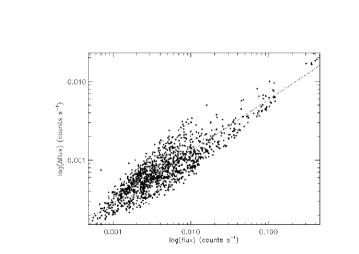
Figure 16: Correlation between $\Delta CR$ and $CR$ for the sources in our sample. The values were obtained from the 0.2-12 keV energy band. The dot-dashed line represents the power law best fit to the points.

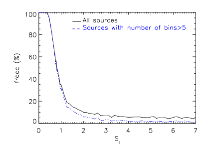
Figure 17: Fraction of simulations that give $S_{o}$ values below $S_{o}^{max}$ as a function of simulated $S_{i}$ for all $CR$, when all sources are used in the simulations (solid line) and when only sources with at least 5 points in their light curves are used (dotted-dashed line).

Finally, for each $cr$ value we obtained the corresponding statistical error from Eq. 11. We then obtained for each simulated light curve the measured values of the intrinsic variability amplitude, $S_{o}$, following the same procedure as for the real data.

For each set of values ($S_{i}$, $CR$) we computed the function $N(S_{o}|S_{i},CR)$ that gives the number of sources with observed amplitude $S_{o}$. Then we calculated the function $N(S_{o}|S_{i})$, that gives for each $S_{i}$ the number of sources in the simulations with value $S_{o}$, weighted with the distribution of $CR$, as

$$N(S_{o}|S_{i})=\sum_{j}P(CR_{j})\times N(S_{o}|S_{i},CR_{j})$$ (12)

where $P(CR)$ is the distribution of count rates in our sources which is shown in Fig. 15. The count rates were obtained as the arithmetic mean of the corrected count rates of all the points in the light curves. The total number of sources in the simulations with observed value $S_{o}$ is

$$N(S_{o})=\sum_{S_{i}}N(S_{o}|S_{i})$$ (13)

$N(S_{o})$ can be used to obtain the probability distribution of $S_{i}$ values for a given $S_{o}$ as

$$P(S_{i}|S_{o})={N(S_{o}|S_{i})\over N(S_{o})}$$ (14)

Then the probability distribution of $S_{i}$ will be

$$P(S_{i})=\sum_{S_{o}}P(S_{i}|S_{o})\times P(S_{o})$$ (15)

where $P(S_{o})$ is the distribution of $S_{o}$ values observed in our sources (see Fig 2).

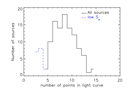
Figure 18: Left: Distribution of the fraction of simulations for each source (for all simulated values of ($S_{i},CR$)) for which $S_{o}\leq S_{o}^{max}$ ($\sim$0.7). Right: Distribution of number of bins in the light curves of our sources. The corresponding distribution for the objects where the fraction of simulations with $S_{o}\leq S_{o}^{max}$ was higher than 10% is indicated with a dashed-line.

In order to get the correct distribution of $P(S_{i})$ we need to simulate up to a value of $S_{i}$ for which all values of $S_{o}$ are above the maximum observed variance $\sigma_{intr}=0.7\equiv S_{o}^{max}$, otherwise the normalisation of $P(S_{i})$ will be wrong. However during the simulations we found a number of sources for which we obtained values of $S_{o}$ below 0.7 independently of how large was the simulated $S_{i}$. This is shown in Fig. 17 where the fraction of these cases is plotted as a function of simulated $S_{i}$ (solid line). Although this fraction decreases rapidly for low $S_{i}$ (below $\sim$2) it remains $\sim$constant for the highest simulated values.

We identified these anomalous cases with sources with a small number of bins in the light curves (see dotted-dashed line in Fig. 17).

Fig. 18 (left) shows the distribution of the fraction of simulations for each source (for all values of ($S_{i},CR$)) for which $S_{o}\leq S_{o}^{max}$ ($\sim$0.7). We see that only a small number of sources have a fraction of $S_{o}\leq S_{o}^{max}$ ($\sim$0.7) above 10%. Fig. 18 (right) shows the distribution of the number of bins in the light curves of our objects (solid line). The corresponding distribution for the sources for which the fraction of simulations with $S_{o}\leq S_{o}^{max}$$\geq$10% is indicated with a dashed-line. Our results show that, selecting a value of the fraction of 10% we pick up most of the “problematic” light curves, withough reducing significantly the number of light curves. In addition we found that these “problematic” cases correspond to the sources with lower number of bins in the light curves.

As we need to simulate values of $S_{i}$ where the fraction of simulations with $S_{o}\leq S_{o}^{max}$ is low, we have not used sources with less than 5 points in their light curves in the calculation of the distributions $P(S_{i})$ and $P(S_{o})$.

This implies that the number of sources for which we can obtain the distribution of $S_{i}$ is 103, instead of the original sample of 120 sources having at least 2 points in their light curves. By doing this selection we can be confident that we can represent the expected distribution of $S_{i}$, $P(S_{i})$, using simulations of $S_{i}$ values up to $\sim 4$.

A fraction of the simulated light curves were found to have negative mean count rates, and therefore in these cases the measured amplitudes of variability, $S_{o}$, were also negative as $S_{o}=\sigma_{Q}/\langle CR\rangle$($\equiv\sigma_{intr}$; see Eq. 3) with $\langle CR\rangle$ being the mean unweighted count rate of the simulated light curve. Our simulations showed that the fraction of simulated light curves with negative mean count rates did not vary significantly with the simulated count rates, $CR$, but it was a strong function of $S_{i}$. This can be seen in Fig. 19 where we plotted this fraction as a function of $S_{i}$ (left) and $CR$ (right). We see that using only simulations with $S_{i}\leq 4$ the maximum fraction of simulated light curves with negative values of $S_{o}$ is $\sim$5% for $S_{i}$=4.

Figure 19: Fraction of simulated light curves with negative mean count rates as a function of $S_{i}$ (intrinsic amplitude; top) and $CR$ (0.2-12 keV count rate; bottom).

This result is expected as for larger values of $S_{i}$ the Gaussian distribution that we are using to obtain simulated count rates becomes broader, while the mean does not move significantly from zero, and hence the probability of obtaining negative average values increases. In all these cases we used the absolute values of the mean count rates to calculate the values of $S_{o}$.