Flat rotation curves using scalar-tensor theories

Abstract

We computed flat rotation curves from scalar-tensor theories in their weak field limit. Our model, by construction, fits a flat rotation profile for velocities of stars. As a result, the form of the scalar field potential and DM distribution in a galaxy are determined. By taking into account the constraints for the fundamental parameters of the theory $(\lambda,\,\alpha)$, it is possible to obtain analytical results for the density profiles. For positive and negative values of $\alpha$, the DM matter profile is as cuspy as NFW’s.

I Introduction

Recently, we have worked on some of the effects that general scalar-tensor theories (STT) of gravity yield on astrophysical scales Ro01 ; RoCe04 ; RoCePeTlCa05 . By taking the weak field limit of STT, three parameters appear PiOb86 : the Newtonian constant at infinity $G_{\infty}$, a Compton length-scale ($\lambda=\hbar/mc$) coming from the effective mass of the Lagrangian potential, and the strength of the new scalar gravitational interaction ($\alpha$). For point-like masses, the new Newtonian potential is of a Yukawa type PiOb86 ; FiTa99 and, in general, analytical expressions can be found for spherical RoCe04 and axisymmetric systems RoCePeTlCa05 . Using these solutions we build a galactic model that is consistent with a flat rotation velocity profile which resembles the observations SoRu01 . In the present short contribution, we outline a way to construct such a galactic model using STT.

II STT and constraints

A typical spiral galaxy consists of a disk, a bulge, and a dark matter (DM) halo. A real halo is roughly spherical in shape and contains most of the matter, up to 90%, of the system. Thus, being the halo the main component, our galactic model will then consist of a spherical system of unknown DM. Therefore, in order compare with observations we assume that test particles –stars and dust– follow DM particles. To construct our halo model, we take the weak field limit of general STT and consider a spherically symmetric fluctuation of the scalar field around some fixed background field. The STT is then characterized by a background value of the scalar field, $\langle\phi\rangle$, a Compton lengthscale, $\lambda$, and a strength $\alpha$ PiOb86 . For point-like sources, the new Newtonian potential is well known to be of a Yukawa type FiTa99 :

$$\Phi_{N}=-\frac{1}{\langle\phi\rangle}\frac{M}{r}(1+\alpha\,\rm{e}^{-r/\lambda})\,.$$ (1)

If one fixes the background field to be the inverse of the Newtonian constant, $\langle\phi\rangle=G_{N}^{-1}$ , then for $r\gg\lambda$ the new Newtonian potential coincides with the standard Newtonian one. Given this, for $r\ll\lambda$ one finds deviations of the order of $(1+\alpha)$ to the Newtonian dynamics. This setting is, however, very constrained by local (solar system) deviations of the Newtonian force, in order for $\alpha$ to be less than $10^{-10}$ FiTa99 . Alternatively, one can choose the setting $\langle\phi\rangle=G_{N}^{-1}(1+\alpha)$ and the new potential coincides with the Newtonian for $r\ll\lambda$ and deviates by $1/(1+\alpha)$ for $r\gg\lambda$. If one thinks of a galactic system, physical scales are around the tens of kiloparsecs –and so is our typical $\lambda$–, then for distances bigger than this, one expects constrictions, e.g. from cluster dynamics or cosmology. Several authors constraints have considered these deviations, giving a rough estimate within the range of $-1<\alpha\lesssim 5$. For example, the value of $\alpha=-0.5$ yields an asymptotic growing factor of $2$ in $G_{N}$, whereas the value of $\alpha=3.0$ reduces $G_{N}$ asymptotically by one fourth.

III The galactic model

For a general density distribution the equations governing the weak energy (Newtonian limit) of STT are He91 ; RoCe04 :

$$\nabla^{2}\Phi_{N} = \frac{G{{}_{N}}}{1+\alpha}\,\left[4\pi\rho-\frac{1}{2}\nabla^{2}\bar{\phi}\right]\;,$$ (2)

$$\nabla^{2}\bar{\phi}-m^{2}\bar{\phi} = -8\pi\alpha\rho\;,$$ (3)

where $\bar{\phi}$ is the scalar field fluctuation and $\rho$ is the density distribution which contains baryons, DM particles, or other types of matter. For definiteness we can think of DM, but its profile is unknown yet. This will be determined by setting the dynamics of test particles, i.e., by demanding the new Newtonian potential to be the one that solves the rotation curves of test particles –stars and dust. That is, we require

$$v_{c}^{2}=r\frac{d\Phi_{N}}{dr}={\rm const.}\,,$$ (4)

where this constant is chosen to fit rotation velocities in spirals SoRu01 ; this is the simplest model. We then proceed to solve for $\Phi_{N}$, and its solution is:

$$\Phi_{N}=v_{c}^{2}\,\ln(r)\,.$$ (5)

Substituting this result into the original system, (2, 3), gives

$$\rho\equiv\rho_{DM}=\frac{v_{c}^{2}}{4\pi G_{N}r^{2}}+\frac{m^{2}}{8\pi(1+\alpha)}\bar{\phi}\,.$$ (6)

For our convenience, we define the following densities: $\rho^{*}\equiv\frac{v_{c}^{2}}{4\pi G_{N}r^{2}}$ and $\rho_{\bar{\phi}}\equiv\frac{m^{2}}{8\pi(1+\alpha)}\bar{\phi}$, where $\rho^{*}$ is the density that the system would have to achieve flat rotation curves if system would be treated solely with Newtonian physics, and $\rho_{\bar{\phi}}$ is the contribution of the scalar field, which should be obtained by integrating the equation:

$$\nabla^{2}\bar{\phi}-\frac{m^{2}}{1+\alpha}\bar{\phi}=-8\pi\alpha\rho^{*}\,.$$ (7)

By comparing (3) with (7), it seems natural to identify $m=m^{*}\sqrt{1+\alpha}$ to convert (7) to a type (3) equation, now for $m^{*}$ and $\rho^{*}$. The solution is therefore given by RoCe04 :

$$\bar{\phi}(r) = 8\pi\alpha a^{2}\left[\frac{\rm{e}^{-r_{a}/\lambda^{*}_{a}}}{r_{a}}\int_{0}^{r_{a}}dx\;x\;\sinh(x/\lambda^{*}_{a})\rho^{*}(x)\right.$$ (8)

$$\left.+\frac{\sinh(r/\lambda^{*}_{a})}{r_{a}}\int_{r_{a}}^{R_{a}}dx\;x\;\rm{e}^{-x/\lambda^{*}_{a}}\rho^{*}(x)\right]\,,$$

where $\lambda^{*}\equiv\lambda\sqrt{1+\alpha}$ and $a$ is a length scale of the spherical system, e.g. related to the distance at which stars possess flat rotation curves; the size of the halo is denoted by $R$. Once (8) is solved, its solution is substituted into (6) to find the DM distribution, $\rho_{DM}$. The procedure outlined here is straightforward. Thus, using our given $\rho^{*}$ the above expression can analytically be integrated to have

$$\bar{\phi}(r) = \frac{2\alpha\,a^{2}v_{c}^{2}}{G_{N}r_{a}}\left[\rm{e}^{-\frac{r_{a}}{\lambda^{*}_{a}}}\,\rm{sinhIntegral}\left(\frac{r_{a}}{\lambda^{*}_{a}}\right)\right.$$ (9)

$$\left.-\rm{sinh}\left(\frac{r_{a}}{\lambda^{*}_{a}}\right)\,\rm{expIntegralEi}\left(-\frac{r_{a}}{\lambda^{*}_{a}}\right)\right]\,.$$

Thus, the DM profile becomes

$$\rho_{DM} = \frac{v_{c}^{2}}{4\pi G_{N}}\left\{\frac{1}{a^{2}r_{a}^{2}}\right.$$ (10)

$$+\frac{\alpha}{1+\alpha}\frac{1}{\lambda_{a}^{2}\,r_{a}}\left[\rm{e}^{-\frac{r_{a}}{\lambda^{*}_{a}}}\,\rm{sinhIntegral}\left(\frac{r_{a}}{\lambda^{*}_{a}}\right)\right.$$

$$\left.\left.-\rm{sinh}\left(\frac{r_{a}}{\lambda^{*}_{a}}\right)\,\rm{expIntegralEi}\left(-\frac{r_{a}}{\lambda^{*}_{a}}\right)\right]\right\}\,.$$

Following, we plot in figure 1 the density profiles $\rho_{DM}$, $\rho^{*}$ and $\rho_{\bar{\phi}}$ for $\lambda=1$, $\alpha=1$. The main contribution to $\rho_{DM}$ comes from $\rho^{*}$, which is an inverse squared function of the radius. The DM profile is therefore cuspy near the galactic centre, similar to the NFW’s obtained from simulations Na96-97 . We have computed the best fits to these curves for $r\ll a$, given by $\rho_{DM}\sim\frac{0.08}{r^{1.99}}$ and $\rho_{\bar{\phi}}\sim\frac{0.06}{r^{0.21}}$. On the other hand, the best fits for $r\gg a$ are $\rho_{DM}\sim\frac{0.16}{r^{2.05}}$ and $\rho_{\bar{\phi}}\sim\frac{0.08}{r^{2.12}}$. In figure 2 we plot the DM profile for various $\lambda$ values, resulting in small changes in the slope. For negative $\alpha$ values, (9) becomes negative, but the DM profile does not become shallower. We have computed the case $\lambda=1.0$, $\alpha=-0.5$ for $r\ll a$ and found $\rho_{DM}\sim\frac{0.08}{r^{2.00}}$, while for $r\gg a$ we obtained $\rho_{DM}\sim\frac{0.02}{r^{1.83}}$.

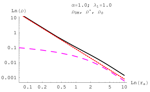
Figure 1: All density profiles as a function of the radius are shown in a log-log scale. The plots were made with $\lambda=1.0$ and $\alpha=1.0$. $\rho_{DM}$ (solid line), $\rho^{*}$ (short-dashed line) and $\rho_{\bar{\phi}}$ (long-dashed line).

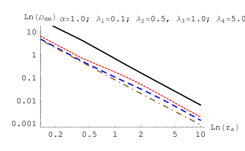
Figure 2: DM density profiles as a function of the radius are shown in log-log scale. The plots were made with $\alpha=1.0$ and $\lambda_{1}=0.1$ (solid line), $\lambda_{2}=0.5$ (short-dashed line), $\lambda_{3}=1.0$ (long-dashed line), and $\lambda_{4}=5.0$ (dashed-dotted line).

IV Conclusions

We have constructed a spherically galactic halo model in which we fit the new gravitational potential to match a flat rotation profile for test particles –stars and dust. Once this is done, one computes the scalar field fluctuation and DM profiles resulting from this potential. We have found analytical results for our model, Eqs.(9) and (10). These equations contain the information of the scalar field ($\lambda$, $\alpha$), which determine the DM profile. We have plotted our results for $\alpha=1.0$ and various $\lambda$s. These profiles have an inner region as cuspy as the NFW’s. Negative values of $\alpha$ do not yield a shallower DM profile neither. This result may however not surprise since we are not resolving the inner structure of the rotation velocity curves. We only considered its flat asymptotic behaviour; in a forthcoming paper we will study it.

Acknowledgements: This work was supported by CONACYT grant numbers 44917 and U47209-F.

References

- (1) Rodríguez–Meza M A, Klapp J, Cervantes–Cota J L, Dehnen H, 2001, in Macias A, Cervantes–Cota J L, Lämmerzahl C, eds, Exact solutions and scalar fields in gravity: Recent developments. Kluwer Academic/Plenum Publishers, New York, p. 213
- (2) Rodríguez–Meza M. A., Cervantes–Cota J. L., 2004, MNRAS 350 671
- (3) Rodríguez–Meza M A et al 2005, Gen. Rel. Grav. 37 823
- (4) Pimentel L O and Obregón O 1986 Astrophys. Space Sci. 126 231-4
- (5) Fischbach E, Talmadge C L, 1999, The search for Non–Newtonian gravity. Springer–Verlag, New York
- (6) Sofue Y and Rubin V 2001 Ann Rev Astron Astrophys 39 137-174
- (7) Nagata R, Chiba T, Sugiyama N 2002 Phys. Rev. D 66 103510; Umezu K, Ichiki K, Yahiro M 2005 Phys. Rev. D 72 044010; Shirata A, Shiromizu T, Yoshida N, Suto Y 2005 Phys. Rev. D 71 064030
- (8) Helbig T 1991 ApJ 382 223
- (9) Navarro J. F. et al 1996 ApJ 462 563; 1997 ApJ 490 493