Monte Carlo simulation of uncoupled continuous-time random walks yielding a stochastic solution of the space-time fractional diffusion equation

Abstract

We present a numerical method for the Monte Carlo simulation of uncoupled continuous-time random walks with a Lévy $\alpha$-stable distribution of jumps in space and a Mittag-Leffler distribution of waiting times, and apply it to the stochastic solution of the Cauchy problem for a partial differential equation with fractional derivatives both in space and in time. The one-parameter Mittag-Leffler function is the natural survival probability leading to time-fractional diffusion equations. Transformation methods for Mittag-Leffler random variables were found later than the well-known transformation method by Chambers, Mallows, and Stuck for Lévy $\alpha$-stable random variables and so far have not received as much attention; nor have they been used together with the latter in spite of their mathematical relationship due to the geometric stability of the Mittag-Leffler distribution. Combining the two methods, we obtain an accurate approximation of space- and time-fractional diffusion processes almost as easy and fast to compute as for standard diffusion processes.

I Introduction

Continuous-time random walks (CTRWs) and fractional diffusion equations (FDEs), or fractional Fokker-Planck equations, have received increasing attention. Metzler and Klafter reviewed analytical and numerical methods to solve fractional equations of diffusive type Metzler and Klafter (2000). In Refs. Sokolov et al., 2001; Zaslavsky, 2002; Barkai, 2002; Meerschaert et al., 2002; Metzler and Klafter, 2004; Flomenbom and Klafter, 2005; Scalas, 2006; Zhang et al., 2006; Langlands, 2006, applications and enhancements of these techniques were presented. The relevance of fractional calculus in the phenomenological description of anomalous diffusion has been discussed within applications of statistical mechanics in physics, chemistry and biology Bouchaud and Georges (1990); Ott et al. (1990); ben Avraham and Havlin (2000); del Castillo-Negrete et al. (2005); Sokolov and Klafter (2006); Dubbeldam et al. (2007a, b) as well as finance Scalas et al. (2000); Mainardi et al. (2000); Mainardi and Gorenflo (2000); Cartea and del Castillo-Negrete (2007a, b); even human travel and the spreading of epidemics were modeled with fractional diffusion Brockmann et al. (2006). A direct Monte Carlo approach to fractional Fokker-Planck dynamics through the underlying CTRW requires random numbers drawn from the Mittag-Leffler distribution. Since sampling the latter was considered troublesome, different schemes to avoid it were proposed. One possibility consists in replacing it with the Pareto distribution—i.e., its asymptotic power-law approximation for $t\to\infty$ Heinsalu et al. (2006); however, as the authors point out, this is limited to long times and an index $\beta$ not close to 1. A more general alternative is based on subordination Gorenflo et al. (2007); Magdziarz et al. (2007); Magdziarz and Weron (2007). Here we present a straightforward Monte Carlo method for the efficient simulation of uncoupled CTRWs using an inversion formula for the Mittag-Leffler distribution and apply it to compute approximate solutions of the Cauchy problem for a generalized diffusion equation that has fractional space and time derivatives.

II Theory

II.1 Continuous-time random walks

A CTRW Montroll and Weiss (1965) is a pure jump process; it consists of a sequence of independent identically distributed (i.i.d.) random jumps (events) $\xi_{i}$ separated by i.i.d. random waiting times $\tau_{i}$,

$$t_{n}=\sum_{i=1}^{n}\tau_{i}\,,\quad\tau_{i}\in\mathbb{R}_{+},$$ (1)

so that the position at time $t\in[t_{n},t_{n+1})$ is given by

$$x(t)=\sum_{i=1}^{n}\xi_{i},\quad\xi_{i}\in\mathbb{R}.$$ (2)

A realization of the process is a piecewise constant function resulting from a sequence of up or down steps with different height and depth; see Fig. 1. Jumps are assumed to happen instantaneously or at least in negligible time. In general, jumps and waiting times depend on each other and they can be described by a joint probability density $\varphi(\xi,\tau)$. The latter appears in the integral equation giving the probability density $p(x,t)$ for the process being in position $x$ at time $t$, conditioned on the fact that it was in position $x=0$ at time $t=0$:

$$p(x,t)=\delta(x)\,\Psi(t)+\int_{-\infty}^{+\infty}\!\!d\xi\int_{0}^{t}\!\!d\tau\,\varphi(\xi,\tau)\,p(x-\xi,t-\tau).$$ (3)

Here the initial condition $x(0)=0$ is contained implicitly in the first term $\delta(x)\Psi(t)$, where we find the complementary cumulative distribution function (survival function)

$$\Psi(t)=1-\int_{-\infty}^{+\infty}d\xi\int_{0}^{t}d\tau\,\varphi(\xi,\tau).$$ (4)

Recently, one of the authors of this paper presented an analytical solution of the integral equation in the uncoupled case—i.e., when $\varphi(\xi,\tau)=\lambda(\xi)\psi(\tau)$, where $\lambda(\xi)$ is the jump marginal density and $\psi(\tau)$ is the waiting time marginal density Scalas et al. (2004a).

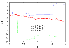
Figure 1: (Color online) Sample paths of CTRWs with scale parameters $\gamma_{t}=0.001,\ \gamma_{x}=\gamma_{t}^{\beta/\alpha}$, and different choices of $\alpha$ and $\beta$. With smaller $\alpha$ the jumps become larger; with smaller $\beta$ the waiting times become longer.

II.2 Fractional diffusion equation

The well-known standard diffusion equation

$$\frac{\partial}{\partial t}u(x,t) = D\frac{\partial^{2}}{\partial x^{2}}u(x,t),$$ (5)

$$u(x,0^{+}) = \delta(x),\quad x\in\mathbb{R},\quad t\in\mathbb{R}_{+},$$

can be generalized to the space-time fractional diffusion equation

$$\frac{\partial^{\beta}}{\partial t^{\beta}}u(x,t) = D\frac{\partial^{\alpha}}{\partial|x|^{\alpha}}u(x,t)$$ (6)

$$u(x,0^{+}) = \delta(x),\quad x\in\mathbb{R},\quad t\in\mathbb{R}_{+},$$

where, for $0<\alpha\leq 2$, $\partial^{\alpha}/\partial|x|^{\alpha}$ denotes the symmetric Riesz-Feller operator of symbol $-|\kappa^{\alpha}|$ and, for $0<\beta\leq 1$, $\partial^{\beta}/\partial t^{\beta}$ is the Caputo derivative Caputo and Mainardi (1971); Saichev and Zaslavsky (1997); Scalas et al. (2004a). Without loss of generality, we assume $D=1$; a different value would just mean a scale transformation of space and/or time units. $u(x,t)\geq 0$ is the Green function of the FDE,

$$u(x,t)=t^{-\beta/\alpha}\,W(x/t^{\beta/\alpha};\,\alpha,\beta),$$ (7)

with the scaling function

$$W(\xi;\,\alpha,\beta)=\mathcal{F}^{-1}_{\kappa}\left[E_{\beta}(-|\kappa|^{\alpha})\right](\xi).$$ (8)

$E_{\beta}(z)$ is the one-parameter Mittag-Leffler function Hilfer and Seybold (2006),

$$E_{\beta}(z)=\sum_{n=0}^{\infty}\frac{z^{n}}{\Gamma(\beta n+1)},\quad z\in\mathbb{C},$$ (9)

with

$$E_{\beta}(-t^{\beta})=\mathcal{L}^{-1}_{s}\left[\frac{s^{\beta-1}}{1+s^{\beta}}\right](t),\quad t\in\mathbb{R}_{+}.$$ (10)

$\mathcal{F}$ and $\mathcal{L}$ denote the Fourier and Laplace transforms:

$$\widehat{f}(\kappa)=\mathcal{F}_{x}[f(x)](\kappa)=\int_{-\infty}^{+\infty}f(x)e^{i\kappa x}\,dx,$$ (11)

$$\widetilde{f}(s)=\mathcal{L}_{t}[f(t)](s)=\int_{0}^{\infty}f(t)e^{-st}\,dt,\quad s\in\mathbb{C}.$$ (12)

For $t\in\mathbb{R}$ and $\beta=1$, the Mittag-Leffler function with argument $-t^{\beta}$ reduces to a standard exponential decay $e^{-t}$; when $0<\beta<1$, the Mittag-Leffler function is approximated for small values of $t$ by a stretched exponential decay (Weibull function) $\exp(-t^{\beta}/a)$, where $a=\Gamma(\beta+1)$, and for large values of $t$ by a power law $bt^{-\beta}$, where $b=\Gamma(\beta)\sin(\beta\pi)/\pi$; see Fig. 2. The Mittag-Leffler distribution is an important example of fat-tailed waiting times; it arises as the natural survival probability leading to time-fractional diffusion equations. There is increasing evidence for physical phenomena Shlesinger et al. (1993); Ward (1998); Mega et al. (2003) and human activities Raberto et al. (2002); Scalas et al. (2004b); Barabási (2005) that do not follow either exponential or, equivalently, Poissonian statistics.

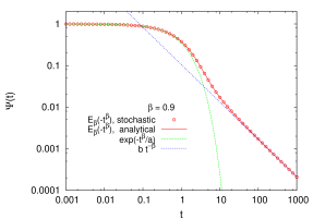
Figure 2: (Color online) The Mittag-Leffler complementary cumulative distribution function sampled from Eq. (20) (circles) and computed analytically (solid line) Podlubny and Kacenak (2005), as well as its approximations for $t\to 0$ (Weibull function, long dashes) and $t\to\infty$ (power law, short dashes).

Equations (7) and (8) can be obtained by Fourier-Laplace transformation of the FDE, recalling the definition of the fractional derivatives used in Eq. (6).

The space-fractional derivative of order $\alpha\in(0,2]$ is defined according to Riesz Samko et al. (1993):

$$\frac{d^{\alpha}}{d|x|^{\alpha}}f(x)=\mathcal{F}^{-1}_{\kappa}\left[-|\kappa|^{\alpha}\widehat{f}(\kappa)\right](x).$$ (13)

For $\alpha=2$ this reduces to the usual second order derivative. For $\alpha<2$ the following equation holds:

$$\frac{d^{\alpha}f(x)}{d|x|^{\alpha}}\!=\!\frac{\Gamma(\alpha\!+\!1)}{\pi}\sin\frac{\alpha\pi}{2}\!\!\int_{0}^{\infty}\!\frac{f(x\!+\!\xi)\!-\!2f(x)\!+\!f(x\!-\!\xi)}{\xi^{\alpha+1}}d\xi.$$ (14)

The time-fractional derivative of order $\beta\in(0,1]$ is defined according to Caputo Gorenflo and Mainardi (1997); Podlubny (1999):

$$\frac{d^{\beta}}{dt^{\beta}}f(t)=\mathcal{L}^{-1}_{s}\left[s^{\beta}\widetilde{f}(s)-s^{\beta-1}f(0^{+})\right](t).$$ (15)

For $\beta=1$ this reduces to the usual first order derivative. For $\beta<1$ the following equation holds:

$$\frac{d^{\beta}f(t)}{dt^{\beta}}=\frac{1}{\Gamma(1-\beta)}\left[\frac{d}{dt}\int_{0}^{t}\frac{f(\tau)}{(t-\tau)^{\beta}}\,d\tau-\frac{f(0^{+})}{t^{\beta}}\right],$$ (16)

where $f(0^{+})$ is the initial condition. For $\alpha=2$ and $\beta=1$, the standard diffusion equation, Eq. (5), is recovered.

It is inevitable to solve numerically a FDE in the most general case, also known as fractional Fokker-Planck equation, which may include space- and time-dependent diffusion and drift terms. Possible approaches are the direct calculation of the integrals in Eqs. (14) and (16) Ford and Connolly (2006), finite-difference methods Meerschaert et al. (2006); Tadjeran et al. (2006); del Castillo-Negrete (2006), and stochastic methods Meerschaert et al. (2002); Zhang et al. (2006); Heinsalu et al. (2006); Magdziarz et al. (2007); Magdziarz and Weron (2007). All of them are complicated, the latter ones mainly because of the supposedly cumbersome generation of Mittag-Leffler random numbers. While this problem has been often worked around in the past, we show how to overcome it, obtaining a fast and accurate method for the Monte Carlo solution of FDEs via uncoupled CTRWs. As a benchmark, we focus our attention on the Cauchy problem defined in Eq. (6), for which an analytical solution given by Eqs. (7) and (8) is available.

II.3 Link between continuous-time random walks and the fractional diffusion equation

The link between CTRWs and time-fractional diffusion was discussed rigorously in Ref. Hilfer and Anton, 1995 in terms of the generalized Mittag-Leffler function $E_{\beta,\beta}(-\tau^{\beta})$.

In order to approximate the Green function in Eq. (7), it is sufficient to simulate CTRWs whose jumps are distributed according to the symmetric Lévy $\alpha$-stable probability density (which reduces to a Gaussian for $\alpha=2$)

$$L_{\alpha}(\xi)=\mathcal{F}^{-1}_{\kappa}\left[\exp\left(-|\gamma_{x}\kappa|^{\alpha}\right)\right](\xi)$$ (17)

and whose waiting times have the probability density

$$\psi_{\beta}(\tau)=-\frac{d}{d\tau}E_{\beta}\left(-(\tau/\gamma_{t})^{\beta}\right),$$ (18)

where $E_{\beta}(z)$ is the one-parameter Mittag-Leffler function given by Eq. (9). Then a weak-limit approximation of the Green function is obtained by rescaling waiting times by a constant $\gamma_{t}$ and jumps by a constant $\gamma_{x}=\gamma_{t}^{\beta/\alpha}$, letting $\gamma_{t}$ (and as a consequence $\gamma_{x}$) vanish, and plotting the histogram for the probability density $p_{\gamma_{x},\gamma_{t}}(x,t;\,\alpha,\beta)$ of finding position $x$ at time $t$ for the rescaled process. This probability density weakly converges to the Green function $u(x,t;\,\alpha,\beta)$. Weak convergence means that for $x=0$ a singularity is always present in $p_{\gamma_{x},\gamma_{t}}(x,t;\,\alpha,\beta)$ at $x=0$ for any finite value of $\gamma_{t}$ and $\gamma_{x}$. This singularity is the term $\delta(x)\Psi(t)$ in Eq. (3) with $\Psi(t)=E_{\beta}(-t^{\beta})$. In the case $\alpha=2$ and $\beta=1$ the CTRWs are normal compound Poisson processes (NCPPs) and, in the diffusive limit, one recovers the Green function for the standard diffusion equation, Eq. (5)—i.e., the Wiener process. This procedure is justified in Refs. Scalas, 2006 and Scalas et al., 2004a. In the latter reference, one can also find a theoretical justification for the Monte Carlo procedure where waiting times are generated according to a power-law distribution; a more complete treatment has been given in Ref. Gorenflo et al., 2007.

III Transformation formulas for non uniform random numbers

The usual methods for generating random numbers with a specific probability density are transformation, also called inversion because it requires the inverse cumulative distribution function Feller (1957), and von Neumann rejection von Neumann (1951). While the latter is more general, the former is usually faster when it is available.

III.1 Symmetric Lévy $\alpha$-stable probability distribution

The symmetric Lévy $\alpha$-stable probability density $L_{\alpha}(\xi)$ for the jumps, Eq. (17), can be calculated by series expansion, which we do not report here, by direct integration Nolan (1997, 1999) or by numerical Fourier transform Mittnik et al. (1999). These methods produce a pointwise representation of the density on a finite interval that can be used for rejection, most efficiently with a lookup table and interpolation. More convenient is the following transformation method by Chambers, Mallows, and Stuck Chambers et al. (1976):

$$\xi_{\alpha}=\gamma_{x}\left(\frac{-\log u\cos\phi}{\cos((1-\alpha)\phi)}\right)^{1-1/\alpha}\frac{\sin(\alpha\phi)}{\cos\phi},$$ (19)

where $\phi=\pi(v-1/2)$, $u,v\in(0,1)$ are independent uniform random numbers, $\gamma_{x}$ is the scale parameter, and $\xi_{\alpha}$ is a symmetric Lévy $\alpha$-stable random number. For $\alpha=2$, Eq. (19) reduces to $\xi_{2}=2\gamma_{x}\sqrt{-\log u}\sin\phi$, i.e. the Box-Muller method for Gaussian deviates. The other two notable limit cases are the Cauchy distribution, with $\alpha=1$ and $\xi_{1}=\gamma_{x}\tan\phi$, and the Lévy distribution, with $\alpha=1/2$ and $\xi_{1/2}=-\gamma_{x}\tan\phi/(2\log u\cos\phi)$.

III.2 One-parameter Mittag-Leffler probability distribution

The probability density $\psi_{\beta}(\tau)$ for the waiting times, Eq. (18), can be computed as a power series from the definition of the one-parameter Mittag-Leffler function, Eq. (9), leading to a pointwise representation on a finite interval; random numbers can then be produced by rejection, again with a lookup table and interpolation. Though CTRW sample paths with a Mittag-Leffler waiting time distribution have appeared in the literature Gorenflo et al. (2004, 2007); Magdziarz et al. (2007); Magdziarz and Weron (2007), so far it has not been recognized in this context that inversion formulas analogous to Eq. (19) are available Devroye (1996); Pakes (1998); Kozubowski (1998); Kozubowski and Rachev (1999); Kozubowski (2000, 2001); Jayakumar (2003); Germano et al. (2006). The most convenient expression is due to Kozubowski and Rachev Kozubowski and Rachev (1999):

$$\tau_{\beta}=-\gamma_{t}\log u\left(\frac{\sin(\beta\pi)}{\tan(\beta\pi v)}-\cos(\beta\pi)\right)^{1/\beta},$$ (20)

where $u,v\in(0,1)$ are independent uniform random numbers, $\gamma_{t}$ is the scale parameter, and $\tau_{\beta}$ is a Mittag-Leffler random number. For $\beta=1$, Eq. (20) reduces to the inversion formula for the exponential distribution: $\tau_{1}=-\gamma_{t}\log u$. Equation (20) and equivalent forms stem from mixture representations of a Mittag-Leffler random variable through an exponential and a stable random variable. The oldest representation is Devroye (1996); Jayakumar (2003)

$$\tau_{\beta}=\tau_{1}^{1/\beta}\,\xi_{\beta,1},$$ (21)

where $\xi_{\beta,1}$ is a skew Lévy $\alpha$-stable random number independent of $\tau_{1}$, with index $\alpha=\beta$, skewness parameter 1, and scale factor $\gamma_{x}=1/8$. A more recent representation is Pakes (1998); Kozubowski (1998)

$$\tau_{\beta}=\tau_{1}\,\xi_{1+}^{\pm 1/\beta},$$ (22)

where $\xi_{1+}$ is a positive random number distributed according to a Cauchy distribution $L_{1+}(\xi)$ with scale parameter $\gamma_{x}=\sin(\beta\pi)$, location parameter $\delta=-\cos(\beta\pi)$, and normalization on $\mathbb{R}_{+}$: $L_{1+}(\xi)=L_{1}(\xi)/\beta$ for $\xi>0$.

The connection of Mittag-Leffler to stable random variables can be obtained in the framework of the theory of geometric stable distributions. A random variable $\xi$ is stable if and only if, for all $n\in\mathbb{N}$ i.i.d. copies of it, $\xi_{1},\ldots,\xi_{n}$, there exist constants $a_{n}\in\mathbb{R}_{+}$ and $b_{n}\in\mathbb{R}$ such that the scaled and shifted sum $a_{n}(\xi_{1}+\cdots+\xi_{n})+b_{n}$ has the same distribution as $\xi$. A Mittag-Leffler random variable is not stable, but it is geometric stable Kotz et al. (2001); i.e., it is the weak limit for $p\to 0$ of the appropriately scaled and shifted geometric random sum $a(p)[\tau_{1}+\cdots+\tau_{\nu(p)}]+b(p)$ of suitable i.i.d. random variables $\tau_{i}$, where $\nu(p)$ is a geometric random variable indepedent of each $\tau_{i}$, with mean $1/p,\ p\in(0,1),$ and a geometric probability distribution

$$P(\nu(p)=n)=p(1-p)^{n-1},\quad n\in\mathbb{N}.$$ (23)

A random variable is geometric stable if and only if its characteristic function $\widehat{\psi}(\kappa)$ is related to the characteristic function $\widehat{\lambda}(\kappa)$ of a stable random variable by the equation Mittnik and Rachev (1991)

$$\widehat{\psi}(\kappa)=\frac{1}{1-\log\widehat{\lambda}(\kappa)}.$$ (24)

With this one-to-one correspondence, a parametrization of a geometric stable probability density $\psi(x)$ can be established from a parametrization of the corresponding stable probability density $\lambda(x)$. Geometric random sums of symmetric $\tau_{i}$ yield the class of Linnik distributions (a generalization of the Laplace distribution $\frac{1}{2}e^{-|t|}$), while positive $\tau_{i}$ yield the class of Mittag-Leffler distributions (as already seen, a generalization of the exponential distribution $e^{-t},\ t\geq 0$). In particular, the Mittag-Leffler distribution can be written as a mixture of exponential distributions Gorenflo and Mainardi (1997); Kozubowski (2001):

$$E_{\beta}(-t^{\beta})=\int_{0}^{\infty}\exp(-\mu t)g(\mu)\,d\mu,$$ (25)

with a weight

$$g(\mu)=\frac{1}{\pi}\frac{\sin(\beta\pi)}{\mu^{1+\beta}+2\cos(\beta\pi)\mu+\mu^{1-\beta}}$$ (26)

given by $g(\mu)d\mu=L_{1+}(\mu^{\beta})d\mu^{\beta}$, where $L_{1+}(\xi)$ is the probability density of $\xi_{1+}$ in Eq. (22) introduced before. Equations (25) and (26) express Eq. (22) in terms of density functions. The inverse cumulative distribution of $L_{1+}(\xi)$ yields the transformation formula for $\xi_{1+}$ appearing as the argument of the power function in Eq. (20) Kozubowski and Rachev (1999); Kozubowski (2000). Alternatively, the inversion formula $\xi_{1}=\gamma_{x}\tan\phi+\delta$ for $L_{1}(\xi)$, see Eq. (19), can be substituted into Eq. (22), provided negative values of $\xi_{1}$ are discarded.

An older equivalent form of Eq. (20) was obtained substituting an inversion formula for $\xi_{\beta,1}$ Kanter (1975) into Eq. (21) Devroye (1996); Jayakumar (2003). A similar result can be reached using a general transformation formula for skew Lévy $\alpha$-stable random numbers Chambers et al. (1976), of which Eq. (19) is a special case with skewness parameter 0. Both ways require three independent uniform random numbers and more transcendent functions than Eq. (20), making the latter slightly more appealing from a numerical point of view.

IV Numerical results

Examples of CTRWs generated according to the described procedure—i.e., Eqs. (1), (2), (19) and (20)—are shown in Fig. 1. The complementary cumulative distribution function (survival function) of random numbers obtained through Eq. (20) is checked against its analytic value Podlubny and Kacenak (2005) and its approximations for $t\to 0$ and $t\to\infty$ in Fig. 2, where a log-log scale and logarithmic binning Newman (2005) is used. Timings are reported in Table 1 and Ref. Germano et al., 2006.

$\alpha$	$\beta$	$\gamma_{t}$	$\bar{n}$	$t_{\mathrm{CPU}}$/sec
2.0	1.0	0.010	200	337
2.0	1.0	0.001	2000	3362
1.7	0.8	0.010	74	437
1.7	0.8	0.001	470	2895

Table 1: Average number $\bar{n}$ of jumps per run and total CPU time $t_{\mathrm{CPU}}$ in seconds for $10^{7}$ runs with $t\in[0,2]$ on a 2.2 GHz AMD Athlon 64 X2 Dual-Core with Fedora Core 4 Linux, using the ran1 uniform random number generator Press et al. (2003) and the Intel C++ compiler version 9.1 with the -O3 -static optimization options.

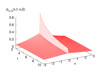
Figure 3: (Color online) Decay of the probability density $p_{\gamma_{x},\gamma_{t}}(x,t;\,\alpha,\beta)$ with $\alpha=1.7,\ \beta=0.8,\ \gamma_{t}=0.1,$ and $\gamma_{x}=\gamma_{t}^{\beta/\alpha}$. The crest at $x=0$ is the survival function $\Psi(t)=E_{\beta}\left(-(t/\gamma_{t})^{\beta}\right)=P(0^{+},t)-P(0^{-},t)$, where $P(x,t)=\int_{-\infty}^{x}p(u,t)\,du$.

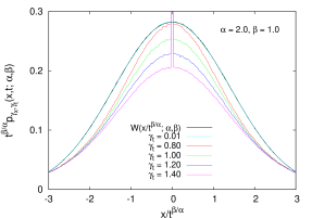
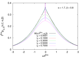
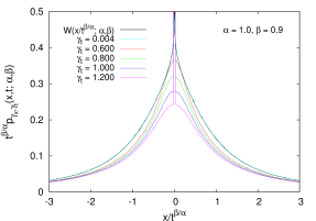
Figure 4: (Color online) Convergence of $t^{\beta/\alpha}p_{\gamma_{x},\gamma_{t}}(x,t;\,\alpha,\beta)$ to the scaling function $W(x/t^{\beta/\alpha};\,\alpha,\beta)$, Eq. (8), at $t=2$ for selected values of $\alpha$ and $\beta$. The curves are shown in a time-independent way as scaling plots and appear in the same order from bottom to top as reported in the legend—i.e., with decreasing $\gamma_{t}$. The curve with the smallest $\gamma_{t}$ is almost indistinguishable from its theoretical limit $W$ (solid black line). However, in spite of the impression that may arise from the few terms and the ranges chosen here, in general the function sequences are not monotonic. The scale parameters $\gamma_{x}$ and $\gamma_{t}$ tend to 0 as $\gamma_{x}^{\alpha}=\gamma_{t}^{\beta}$. The central peak decreases when the ratio $t/\gamma_{t}$ becomes larger, as is evident in Fig. 3.

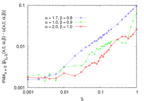
Figure 5: (Color online) Convergence of $\max_{x\neq 0}|p_{\gamma_{x},\gamma_{t}}(x,t;\,$ $\alpha,\beta)-u(x,t;\,\alpha,\beta)|$ for selected values of $\alpha$ and $\beta$ when $\gamma_{x},\ \gamma_{t}\to 0$ with $\gamma_{x}^{\alpha}=\gamma_{t}^{\beta}$.

The advantage of Eq. (20) is that Mittag-Leffler deviates are generated with a simple and elegant procedure and no accuracy losses due to truncation of the power series in Eq. (9) or truncation of the density function to a finite interval as necessary in the rejection method. The effects of the truncation of the jump density in Lévy flights are analyzed in Ref. Mantegna and Stanley, 1994, whereas no study is available for truncation effects on Mittag-Leffler deviates. Together with Eq. (19), a scheme is obtained that yields sample paths for a CTRW with a Lévy jump marginal density and a Mittag-Leffler waiting time marginal density at a speed comparable to that of a NCPP: Though each point for a generic CTRW takes about 3.6 times more than for a NCPP, fewer points are necessary (see $\bar{n}$ in Table 1) because the waiting times are longer. The latter reference reports also that if Lévy and Mittag-Leffler random numbers are produced by rejection, computing the values of the probability density functions simple-mindedly with a series expansion every time they are needed, rather than just once at the beginning to set up a lookup table, for Lévy deviates the procedure takes 400 times longer than with Eq. (19) and for Mittag-Leffler deviates it takes 5000 times longer than with Eq. (20). Because of the slow convergence of the power series in Eq. (9), up to 200 terms are necessary to achieve an acceptable accuracy, and each term is computationally expensive because of the $\Gamma$ function. Of course these are extreme figures on the other end of the efficiency scale meant to show how wide the latter can be; there are smarter ways to compute both the Lévy and Mittag-Leffler Podlubny (1999); Podlubny and Kacenak (2005) probability densities.

Using many CTRW realizations, histograms can be built that give the evolution of $p(x,t)$ with initial condition $p(x,0)=\delta(x)$, as displayed in Fig. 3. According to Eq. (3), the initial condition evolves as $\delta(x)\Psi(t)$; i.e., it is visible as a spike at $x=0$ that decays as $t$ evolves. The mass of the spike is $\Psi(t)=E_{\beta}\left(-(t/\gamma_{t})^{\beta}\right)$. In Fig. 3 this feature appears as a crest. Figure 4 shows how histograms built with CTRWs converge to the Green function, Eq. (7), of the FDE for decreasing values of the scale parameters $\gamma_{t}$ and $\gamma_{x}=\gamma_{t}^{\beta/\alpha}$. To evaluate the scaling function in Eq. (8) needed for Eq. (7), we used standard algorithms for $E_{\beta}(-t^{\beta})$ Podlubny (1999); Raberto et al. (2002); Podlubny and Kacenak (2005), including the fast Fourier transform. In Fig. 5 we plot $\max_{x\neq 0}|p_{\gamma_{x},\gamma_{t}}(x,t;\,\alpha,\beta)-u(x,t;\,\alpha,\beta)|$ as a function of vanishing $\gamma_{t}$ with $\gamma_{x}=\gamma_{t}^{\beta/\alpha}$. A rigorous analysis of convergence bounds is beyond the scope of this paper.

V Conclusions

The use of Mittag-Leffler random numbers generated according to Eq. (20) in combination with Lévy random numbers generated according to Eq. (19) is very useful in the Monte Carlo simulation of uncoupled continuous-time random walks. In the hydrodynamic limit, appropriately rescaled uncoupled continuous-time random walks with a one-parameter Mittag-Leffler distribution of waiting times and a symmetric Lévy $\alpha$-stable distribution of jumps in space yield the Green function of the Cauchy problem for a space-time fractional diffusion equation; we verified this for Eq. (6), which has an analytical solution, Eq. (7), as a benchmark for more difficult cases where the diffusion and drift terms depend on space and time. We have shown that the computational effort for a fractional diffusion process is almost as small as for a standard diffusion process. It is true that in the same fluid limit the Green function can be obtained too by Monte Carlo sampling of just the asymptotic power-law tail approximations of the Lévy and Mittag-Leffler probability distributions, at least when the indices $\alpha$ and $\beta$ are not close to 2 and 1, respectively. However, the neat transformation formulas given by Eqs. (19) and (20) are numerically so convenient that there is no good reason for resorting to the asymptotic approximations. Moreover, we think that, in applications, continuous-time random walks are seen as a more fundamental model than fractional diffusion equations, and sample paths will be generated without taking the scale parameters $\gamma_{x}$ and $\gamma_{t}$ to the diffusive limit, by using the approach presented in this paper.

References

- Metzler and Klafter (2000) R. Metzler and J. Klafter, Phys. Rep. 339, 1 (2000).
- Sokolov et al. (2001) M. Sokolov, A. Blumen, and J. Klafter, Physica A 302, 268 (2001).
- Zaslavsky (2002) G. M. Zaslavsky, Phys. Rep. 371, 461 (2002).
- Barkai (2002) E. Barkai, Chem. Phys. 284, 13 (2002).
- Meerschaert et al. (2002) M. M. Meerschaert, D. A. Benson, H.-P. Scheffler, and B. Baeumer, Phys. Rev. E 65, 041103 (2002).
- Metzler and Klafter (2004) R. Metzler and J. Klafter, J. Phys. A: Math. Gen. 37, R161 (2004).
- Flomenbom and Klafter (2005) O. Flomenbom and J. Klafter, Phys. Rev. Lett. 95, 098105 (2005).
- Scalas (2006) E. Scalas, Physica A 362, 225 (2006).
- Zhang et al. (2006) Y. Zhang, D. A. Benson, M. M. Meerschaert, E. M. LaBolle, and H.-P. Scheffler, Phys. Rev. E 74, 026706 (2006).
- Langlands (2006) T. A. M. Langlands, Physica A 367, 135 (2006).
- Bouchaud and Georges (1990) J.-P. Bouchaud and A. Georges, Phys. Rep. 195, 127 (1990).
- Ott et al. (1990) A. Ott, J.-P. Bouchaud, D. Langevin, and W. Urbach, Phys. Rev. Lett. 65, 2201 (1990).
- ben Avraham and Havlin (2000) D. ben Avraham and S. Havlin, Diffusion and Reactions in Fractals and Disordered Systems (Cambridge University Press, Cambridge, England, 2000).
- del Castillo-Negrete et al. (2005) D. del Castillo-Negrete, B. A. Carreras, and V. E. Lynch, Phys. Rev. Lett. 94, 065003 (2005).
- Sokolov and Klafter (2006) I. M. Sokolov and J. Klafter, Phys. Rev. Lett. 97, 140602 (2006).
- Dubbeldam et al. (2007a) J. L. A. Dubbeldam, A. Milchev, V. G. Rostiashvili, and T. A. Vilgis, Phys. Rev. E 76, 010801(R) (2007a).
- Dubbeldam et al. (2007b) J. L. A. Dubbeldam, A. Milchev, V. G. Rostiashvili, and T. A. Vilgis, Europhys. Lett. 79, 18002 (2007b).
- Scalas et al. (2000) E. Scalas, R. Gorenflo, and F. Mainardi, Physica A 284, 376 (2000).
- Mainardi et al. (2000) F. Mainardi, M. Raberto, R. Gorenflo, and E. Scalas, Physica A 287, 468 (2000).
- Mainardi and Gorenflo (2000) F. Mainardi and R. Gorenflo, J. Comput. Appl. Math. 118, 283 (2000).
- Cartea and del Castillo-Negrete (2007a) A. Cartea and D. del Castillo-Negrete, Physica A 374, 749 (2007a).
- Cartea and del Castillo-Negrete (2007b) A. Cartea and D. del Castillo-Negrete, Phys. Rev. E 76, 041105 (2007b).
- Brockmann et al. (2006) D. Brockmann, L. Hufnagel, and T. Geisel, Nature 439, 462 (2006).
- Heinsalu et al. (2006) E. Heinsalu, M. Patriarca, I. Goychuk, G. Schmid, and P. Hänggi, Phys. Rev. E 73, 046133 (2006).
- Gorenflo et al. (2007) R. Gorenflo, F. Mainardi, and A. Vivoli, Chaos Soliton Fract. 34, 87 (2007).
- Magdziarz et al. (2007) M. Magdziarz, A. Weron, and K. Weron, Phys. Rev. E 75, 016708 (2007).
- Magdziarz and Weron (2007) M. Magdziarz and A. Weron, Phys. Rev. E 75, 056702 (2007).
- Montroll and Weiss (1965) E. W. Montroll and G. H. Weiss, J. Math. Phys. 6, 167 (1965).
- Scalas et al. (2004a) E. Scalas, R. Gorenflo, and F. Mainardi, Phys. Rev. E 69, 011107 (2004a).
- Caputo and Mainardi (1971) M. Caputo and F. Mainardi, Riv. Nuovo Cimento 1, 161 (1971).
- Saichev and Zaslavsky (1997) A. I. Saichev and G. M. Zaslavsky, Chaos Soliton Fract. 7, 753 (1997).
- Hilfer and Seybold (2006) R. Hilfer and H. J. Seybold, Integr. Transf. Spec. F. 17, 637 (2006).
- Shlesinger et al. (1993) M. F. Shlesinger, G. M. Zaslavsky, and J. Klafter, Nature 363, 31 (1993).
- Ward (1998) S. N. Ward, Nature 394, 827 (1998).
- Mega et al. (2003) M. S. Mega, P. Allegrini, P. Grigolini, V. Latora, L. Palatella, A. Rapisarda, and S. Vinciguerra, Phys. Rev. Lett. 90, 188501 (2003).
- Raberto et al. (2002) M. Raberto, E. Scalas, and F. Mainardi, Physica A 314, 749 (2002).
- Scalas et al. (2004b) E. Scalas, R. Gorenflo, H. Luckock, F. Mainardi, M. Mantelli, and M. Raberto, Quant. Finance 4, 695 (2004b).
- Barabási (2005) A.-L. Barabási, Nature 435, 207 (2005).
- Podlubny and Kacenak (2005) I. Podlubny and M. Kacenak, Mittag-Leffler function — Calculates the Mittag-Leffler function with desired accuracy (2005), MATLAB Central File Exchange, file ID 8738, mlf.m, URL http://www.mathworks.com/matlabcentral/fileexchange.
- Samko et al. (1993) S. G. Samko, A. A. Kilbas, and O. I. Marichev, Fractional Integrals and Derivatives, Theory and Applications (Gordon and Breach Science Publishers, London, 1993).
- Gorenflo and Mainardi (1997) R. Gorenflo and F. Mainardi, in Fractals and Fractional Calculus in Continuum Mechanics, edited by A. Carpinteri and F. Mainardi (Springer, New York, 1997), pp. 223–276, vol. 378 of CISM Courses and Lectures, URL http://www.fracalmo.org.
- Podlubny (1999) I. Podlubny, Fractional Differential Equations (Academic Press, San Diego, 1999).
- Ford and Connolly (2006) N. J. Ford and J. A. Connolly, Commun. Pure Appl. Anal. 5, 289 (2006).
- Meerschaert et al. (2006) M. M. Meerschaert, H.-P. Scheffler, and C. Tadjeran, J. Comput. Phys. 211, 249 (2006).
- Tadjeran et al. (2006) C. Tadjeran, M. M. Meerschaert, and H.-P. Scheffler, J. Comput. Phys. 213, 205 (2006).
- del Castillo-Negrete (2006) D. del Castillo-Negrete, Phys. Plasmas 13, 082308 (2006).
- Hilfer and Anton (1995) R. Hilfer and L. Anton, Phys. Rev. E 51, R848 (1995).
- Feller (1957) W. Feller, An Introduction to Probability Theory and its Applications (John Wiley, New York, 1957).
- von Neumann (1951) J. von Neumann, NBS Appl. Math. Ser. 12, 36 (1951).
- Nolan (1997) J. Nolan, Commun. Stat. Stoch. Models 13, 759 (1997).
- Nolan (1999) J. Nolan, Math. Comput. Modell. 29, 229 (1999).
- Mittnik et al. (1999) S. Mittnik, T. Doganoglu, and D. Chenyao, Math. Comput. Modell. 29, 235 (1999).
- Chambers et al. (1976) J. M. Chambers, C. L. Mallows, and B. W. Stuck, J. Am. Stat. Assoc. 71, 340 (1976).
- Gorenflo et al. (2004) R. Gorenflo, A. Vivoli, and F. Mainardi, Nonlinear Dynam. 38, 101 (2004).
- Devroye (1996) L. Devroye, in Proceedings of the 1996 Winter Simulation Conference, edited by J. M. Charnes, D. J. Morrice, D. T. Brunner, and J. J. Swain (IEEE Press, New York, 1996), pp. 265–272.
- Pakes (1998) A. G. Pakes, Stat. Probab. Lett. 37, 213 (1998).
- Kozubowski (1998) T. J. Kozubowski, Stat. Probab. Lett. 38, 157 (1998).
- Kozubowski and Rachev (1999) T. J. Kozubowski and S. T. Rachev, J. Comput. Anal. Appl. 1, 177 (1999).
- Kozubowski (2000) T. J. Kozubowski, J. Comput. Appl. Math. 116, 221 (2000).
- Kozubowski (2001) T. J. Kozubowski, Math. Comput. Model. 34, 1023 (2001).
- Jayakumar (2003) K. Jayakumar, Math. Comput. Model. 37, 1427 (2003).
- Germano et al. (2006) G. Germano, M. Engel, and E. Scalas, in Proceedings of the 1st International Workshop on Grid Technology for Financial Modeling and Simulation, edited by S. Cozzini, S. d’Addona, and R. Mantegna (SISSA, Trieste, 2006), PoS(GRID2006)011, URL http://pos.sissa.it.
- Kotz et al. (2001) S. Kotz, T. J. Kozubowski, and K. Podgorski, The Laplace Distribution and Generalizations: A Revisit with Applications to Communications, Economics, Engineering, and Finance (Birkhäuser, Boston, 2001).
- Mittnik and Rachev (1991) S. Mittnik and S. T. Rachev, in Stable Processes and Related Topics, edited by S. Cambanis, G. Samorodnitsky, and M. S. Taqqu (Birkhäuser, Boston, 1991), pp. 107–119.
- Kanter (1975) M. Kanter, Ann. Probab. 3, 697 (1975).
- Newman (2005) M. E. J. Newman, Contemp. Phys. 46, 323 (2005).
- Press et al. (2003) W. H. Press, S. A. Teukolsky, W. T. Vetterling, and B. P. Flannery, Numerical Recipes in C++ (Cambridge University Press, Cambridge, England, 2003), 2nd ed.
- Mantegna and Stanley (1994) R. N. Mantegna and H. E. Stanley, Phys. Rev. Lett. 73, 2946 (1994).