Electric-field-enhanced transport in polyacrylamide hydrogel nano-composites

Abstract

Electroosmotic pumping through uncharged hydrogels can be achieved by embedding the polymer network with charged colloidal inclusions. Matos et al. (2006) recently used the concept to enhance the diffusion-limited flux of uncharged molecules across polyacrylamide hydrogel membraness for the purpose of improving the performance of biosensors. This paper seeks to link their reported macroscale diagnostics to physicochemical characteristics of the composite microstructure. The experiments are characterized by a Debye screening length that is much larger than the radius of the silica nanoinclusions and the Brinkman screening length of the polymer skeleton. Accordingly, closed-form expressions for the incremental pore mobility are derived, and these are evaluated by comparison with numerically exact solutions of the full electrokinetic model. A mathematical model for the bulk electroosmotically enhanced tracer flux is proposed, which is combined with the electrokinetic model to ascertain the electroosmotic pumping velocity from measured flux enhancements. Because the experiments are performed with a known current density, but unknown bulk conductivity and electric field strength, theoretical estimates of the bulk electrical conductivity are adopted. These account for nano-particle polarization, added counterions, and non-specific adsorption. Theoretical predictions of the flux enhancement, achieved without any fitting parameters, are within a factor of two of the experiments. Alternatively, if the Brinkman screening length of the polymer skeleton is treated as a fitting parameter, then the best-fit values are bounded by the range 0.9–1.6 nm, depending on the inclusion size and volume fraction. Independent pressure-driven flow experiments reported in the literature for polyacrylamide gels without inclusions suggest 0.4 or 0.8 nm. The comparison can be improved by allowing for hindered ion migration, while uncertainties regarding the inclusion surface charge are demonstrated to have a negligible influence on the electroosmotic flow. Finally, and perhaps most importantly, anomalous variations in the flux enhancement with particle size and volume fraction can be rationalized at present only by acknowledging that particle-particle and particle-polymer interactions increase the effective permeability of the hydrogel skeleton. This bears similarities to the increase in polymer free volume that accompanies the addition of silica nanoparticles to certain polymeric membranes.

1 Introduction

Electric fields are widely used to probe the physicochemical characteristics of dispersed colloidal particles. Microelectrophoresis, capillary electrophoresis and gel electrophoresis, for example, are routinely used to characterize and sort DNA fragments, proteins, synthetic and biological macromolecules, and supramolecular aggregates. In all these applications, the electric field induces translation (electrophoresis) of charged particles, with the electrophoretic velocity reflecting a balance of electrical, hydrodynamic and steric interaction forces, which, in turn, are related to the particle size and charge, and properties of the dispersing medium.

Matos et al. (2006) recently proposed a novel means of promoting the transfer of uncharged molecules across uncharged polyacrylamide hydrogels. By embedding the polymer skeleton with immobilized silica nanoparticles, they endowed the matrix with a fixed charge, and demonstrated that the application of an electric field enhanced the otherwise diffusion-limited flux of uncharged tracer across the membrane. Despite the possibility of promoting unwanted electrostatic interactions with charged molecules, the ability to control the effective charge density by varying the concentration of immobilized inclusions offers several advantages over chemical and/or physicochemical modifications of the polymer architecture alone. Specific interactions may also be imparted by decorating the inclusions with functional moieties, such as in affinity chromotography.

As expected from studies involving electroosmotic microfluidic pumping (Yao and Santiago, 2003; Yao et al., 2003), enhanced transport in immobilized cell culture (Chang et al., 1995) and electroosmotic dewatering (Yukawa et al., 1976), the origin of the electric-field induced flux enhancement in Matos et al.’s experiments was qualitatively attributed to electroosmotic flow originating from the diffuse layers of charge that envelop the silica inclusions. Moreover, the microstructure of the composites synthesized by Matos et al. has potential to serve as a model system with which to test electrokinetic theory that predicts, from first principles, the average electroosmotic pumping velocity, electrical conductivity, and effective ion diffusion coefficients in this novel class of nano-structured composites (Hill, 2006c, d). Indeed, the purpose of this paper is to provide a quantitative theoretical interpretation of the available experiments and, in turn, link macroscale diagnostics to characteristics of the microstructure.

The paper is set out as follows. First, a detailed description of Matos et al.’s experiments is provided in §2. This identifies the relevant parameters and highlights the available diagnostics. Section 3 presents various aspects of the theory. In particular, §§3.1 describes the electrokinetic model; §§3.2 derives the means of linking Matos et al.’s flux enhancement ratio to the electroosmotic pumping velocity; §§3.3 addresses the bulk electrical conductivity of the composite membranes; and §§3.4 evaluates—by comparison with numerical solutions of the full electrokinetic model—a convenient closed-form approximation for the incremental pore mobility. The results are presented in §4. Here, literature values of the permeability of gels without inclusions—obtained from pressure-driven flows—are compared to values inferred from the electrokinetic interpretation of the experiments. Certain anomalies are discussed in §5, and the paper concludes with a summary (§6).

2 Experimental

The hydrogel nanocomposite membranes synthesized in Matos et al.’s experiments comprise a polyacrylamide hydrogel matrix with silica nanosphere inclusions. The hydrogels were synthesized with a polymer mass fraction $c=0.15$ (mass of polymer to mass of water). After polymerization and cross-linking, however, the matrix was reported to swell, yielding a final polymer mass fraction $c\approx 0.13$. The microstructure of the membranes is characterized by the radius of the inclusions ($a\approx 3.5$ or $7.5$ nm) and the inclusion volume fraction ($\phi\approx 0.02$ or $0.04$).

A schematic illustration of Matos et al.’s apparatus is presented in figure 1. The membrane comprises 29 cylindrical sub-membranes, each with a diameter 2.68 mm (giving a total cross-sectional area $A\approx 1.64$ cm²) and thickness $L\approx 1.68$ mm. Matos et al. measured the diffusion coefficient of the tracer (amino-methylcoumarin) in gel membranes with and without inclusions, establishing a value $D\approx 3.3\times 10^{-10}$ m²s^-1. They did not discern the $O(\phi)\ll 1$ influence of the impenetrable inclusions on the effective diffusion coefficient.

The experiments were initiated by establishing a quasi-steady diffusive flux of uncharged tracer across each membrane before applying a potential difference to the electrodes. The electric field was applied after 30 min, which is short compared to the characteristic diffusion time scale $L^{2}/D\approx 140$ min. However, it is evident from the experiments and, indeed, the exact solution of the transient diffusion problem (Matos et al., 2006), that the fastest transients decay in about 30 min.

Figure 1: Schematic of the experimental apparatus used by Matos et al. (2006) to measure the electric-field enhanced flux of a neutral tracer across polyacrylamide hydrogel-silica nanocomposite membranes. The immobilized silica nanoinclusions endow the microstructure with a negative charge, which, with an electric field $E=-\mbox{d}\psi/\mbox{d}x$ between the electrodes, drives electroosmotic flow from the anode ($+$, left) toward the cathode ($-$, right). The flow produces a convective enhancement of the otherwise purely diffusive flux of the neutral tracer, whose concentration is denoted $n^{\infty}(x)$, from the source resevoir to the sink resevoir. See the text and Matos et al.’s paper for details.

The gold electrodes, which present a circular surface area on each side of the membrane, have a diameter 1.9 cm and are separated by a distance 6 mm. In the experiments considered in this paper, the differential voltage was controlled to maintain a constant electrical current $i\approx 3$ mA.

The experiments were performed with the source and the sink reservoirs initially filled with either 1 mmol l^-1KNO₃ electrolyte or deionized (DI) water. Only the source reservoir contained tracer (with concentration 0.1 mmol l^-1) at the beginning of the experiments, and the electrolytes on each side of the membrane were recirculated at a rate $Q\approx 8$ cm³ min^-1, with respective source and sink reservoir volumes $V_{1}\approx 50$ cm³ and $V_{2}\approx 10$ cm³.

The residence time of fluid in the two gaps between the membrane and the electrode is $\delta t\approx 3.6$ s, so the thickness of a diffusive boundary layer at the membrane surface is $\delta l\approx\sqrt{\delta tD}\approx 35~{}\mu$m. Equating the diffusive flux across the membrane $D\Delta n^{\infty}/L$ to the flux across the boundary layer $D\delta n^{\infty}/\delta l$ indicates that $\delta n^{\infty}/\Delta n^{\infty}=\delta l/L\sim 10^{-2}$, so the tracer concentration at the edges of the membrane is approximately equal to the bulk concentration in the respective reservoir. Note that the hold-up time of the tracer in the reservoirs is less than $V_{1}/Q\approx 6$ min, which is short compared to the $\sim V_{2}L/(AD)$ characteristic time scale for the (diffusive) tracer flux to change the reservoir concentration by an $O(1)$ amount. It follows that the membrane and reservoir dynamics are quasi-steady.

The tracer (amino-methylcoumarin) concentration was measured with a fluorescence spectrophotometer that continuously sampled fluid in the sink reservoir circuit. Matos et al. also measured the pH in both reservoirs, showing that the source and sink reservoirs, respectively, attain acidic and basic pH with the application of an electric field.

Note that the tracer has an acid dissociation constant $K_{a}=10^{-5}$ mol l^-1, so the fraction of it in a protonated state, $1/(1+K_{a}/[\mbox{H${}_{3}$0${}^{+}$}])$, is significant only when $\mbox{pH}<5$. These conditions prevail in the source reservoir and, possibly, throughout the composite membrane, suggesting that electrophoresis of the tracer should contribute to the net electric-field-induced flux enhancement. From the diffusion coefficient $D\approx 3.3\times 10^{-10}$ m² s^-1, the electrophoretic mobility is (to a first approximation) $eD/(kT)\approx 1.1$ ($\mu$m s^-1)/(V cm^-1). Therefore, with a representative electric field $E\sim 10$ V cm^-1, the electrophoretic velocity of the tracer is $U_{t}\sim 10$ $\mu$m s^-1, which corresponds to $\mbox{Pe}=U_{t}L/D\sim 55$. This is significantly greater than the values ascertained from electroosmotic pumping, suggesting that the flux of protonated tracer might be dominated by electrophoresis. However, the experimental evidence is that the flux is dominated by electro-osmosis (Matos et al., 2006). It follows that $\mbox{pH}>5$ in a significant portion of the composite hydrogel membranes.

Finally, from the tracer concentration time series, Matos et al. reported averaged flux enhancement ratios, which they defined as the ratio of the tracer concentration in the sink reservoir after 300 min (with an electric field applied after the first 30 min) to the concentration from an experiment without an electric field. They appropriately termed this ratio an enhancement factor, whereas the analysis undertaken in this paper approximates it as a flux enhancement factor, $J/J_{0}$. The ratio of the fluxes, which undoubtedly exhibit weak transients, are therefore assumed to be constant in this work. It is evident that individual experiments reflect significant, non-systematic statistical variations, so the analysis below relies entirely on five averaged values of the reported enhancement factor, each with various particle radius $a$ and volume fraction $\phi$, and electrolyte (1 mmol l^-1KNO₃ or deionized water), but fixed membrane geometry and electrical current.

3 Theory

3.1 Electrokinetic model and electoroosmotic flow in uniform composites

The electrokinetic transport model adopted in this work is described in considerable detail elsewhere (Hill, 2006d). Briefly, it comprises the non-linear Poisson Boltzman equation for electrostatics; electrolyte conservation equations involving diffusion, electromigration and convection; and Brinkman’s equations (with an electrical body force) for solvent mass and momentum conservation (Brinkman, 1947). A solution of the equations, with a single spherical charged, impenetrable colloid embedded in an unbounded, rigid polymer gel yields the far-field ($r\rightarrow\infty$) decays of the electrostatic potential $\psi$, ion concentrations $n_{j}$ and fluid velocity $u$. Of prime importance in this paper are perturbations to equilibrium that arise from a uniform electric field $E$. In the far-field, these take the following asymptotic forms:

$$\psi \rightarrow -\mbox{\boldmath$E$\unboldmath}\cdot\mbox{\boldmath$r$\unboldmath}+(\mbox{\boldmath$E$\unboldmath}\cdot\mbox{\boldmath$e$\unboldmath}_{r})D^{E}r^{-2}$$ (1)

$$n_{j} \rightarrow n_{j}^{\infty}+(\mbox{\boldmath$E$\unboldmath}\cdot\mbox{\boldmath$e$\unboldmath}_{r})C^{E}_{j}r^{-2}$$ (2)

$$u \rightarrow -2C^{E}r^{-3}(\mbox{\boldmath$E$\unboldmath}\cdot\mbox{\boldmath$e$\unboldmath}_{r})\mbox{\boldmath$e$\unboldmath}_{r}-C^{E}r^{-3}(\mbox{\boldmath$E$\unboldmath}\cdot\mbox{\boldmath$e$\unboldmath}_{\theta})\mbox{\boldmath$e$\unboldmath}_{\theta}.$$ (3)

Note that $\mbox{\boldmath$e$\unboldmath}_{r}$ and $\mbox{\boldmath$e$\unboldmath}_{\theta}$ are radial and tangential unit vectors, with the polar axis $\mbox{\boldmath$e$\unboldmath}_{z}$ being colinear with $E$. The scalar coefficients $D^{E}$, $C_{j}^{E}$ and $C^{E}\eta/{\ell}^{2}$ are, respectively, the dipole strengths of the electrostatic potential, ion concentrations, and pressure perturbations induced by the forcing $E$. In general, these so-called asymptotic coefficients are complicated functions of the particle radius and $\zeta$-potential, $a$ and $\zeta$, the electrolyte viscosity and Debye screening length, $\eta$ and $\kappa^{-1}$, and the Darcy permeability of the polymer skeleton ${\ell}^{2}$ (square of the Brinkman screening length).

The single-particle problem leads to averaged equations that quantify the bulk ion fluxes and fluid flow in a dilute ($\phi[1+(\kappa a)^{-1}]^{3}\ll 1$) composite (Hill, 2006d). For the statistically uniform composites addressed in this work, the pressure and bulk ion concentration gradients are zero. Accordingly, with a uniform electric field and unidirectional flow and electrolyte and tracer fluxes, the average fluid velocity is

$$U=-\phi(3/a^{3})EC^{E},$$ (4)

where $\phi\ll 1$ is the inclusion volume fraction, and the average ion fluxes are

$$J_{j}=n_{j}^{\infty}U+z_{j}e\frac{D_{j}}{kT}n_{j}^{\infty}E+\phi(3/a^{3})z_{j}e\frac{D_{j}}{kT}n_{j}^{\infty}ED^{E}+\phi(3/a^{3})D_{j}EC_{j}^{E},$$ (5)

where $z_{j}=\pm z$ ($j=1,2$) are the electrolyte ion valences, $D_{j}$ are the ion diffusion coefficients, $kT$ is the thermal energy, and $e$ is the fundamental charge. In Eqn. (5), the first two terms are, respectively, the convective and electromigrative fluxes that prevail in the absence of inclusions; and the last two terms are (microscale) electromigrative and diffusive contributions to the bulk flux arising from disturbances of the inclusions.

3.2 Uncharged tracer flux and flux enhancement

The flux of uncharged tracer is

$$J=n^{\infty}U-DB+\phi(3/a^{3})DC_{3}^{B}B,$$ (6)

where $C_{3}^{B}=(1/2)a^{3}$ and $B=\mbox{d}n^{\infty}/\mbox{d}x$ is the bulk concentration gradient (Hill, 2006c).

Clearly, the electric-field-induced flow $U$ and electrolyte ion fluxes $J_{1}$ and $J_{2}$ are decoupled from the tracer, but the tracer flux is influenced by the electroosmotic flow. Therefore, the tracer concentration satisfies the conservation equation

$$\partial n^{\infty}/\partial t=-\partial J/\partial x,$$ (7)

where

$$J=n^{\infty}U-D[1-(3/2)\phi]\partial n^{\infty}/\partial x.$$ (8)

Under quasi-steady conditions ($\partial n^{\infty}/\partial t\approx 0$), which will be justified shortly, the flux may be written in terms of the tracer concentration at the edges ($x=0$ and $L$) of the membrane:

$$J=U[n^{\infty}(x=L)-n^{\infty}(x=0)e^{\mbox{Pe}}]/(1-e^{\mbox{Pe}}).$$ (9)

Here, the Péclet number is

$$\mbox{Pe}=UL/D=\phi MEL/D$$ (10)

and

$$M\equiv U/(E\phi)=-(3/a^{3})C^{E}[\kappa a,\zeta e/(kT),\kappa{\ell}]$$ (11)

is termed the incremental pore mobility.

Scaling arguments that also consider transients in the tracer concentration in the (well mixed) source and sink indicate that a quasi-steady approximation is reasonable when $V/(LA)\gg 1$ and $\mbox{Pe}\sim 1$; otherwise, $1\ll\mbox{Pe}\ll V/(LA)$ or $LA/V\ll\mbox{Pe}\ll 1$. Here, $V$ is the smallest of the source and sink volumes. For Matos et al.’s experiments, $V\sim 10$ cm³, $A\sim 1$ cm² and $L\sim 0.1$ cm, so $V/(LA)\sim 10\gg 1$, as required when $\mbox{Pe}\sim 1$.

With zero electric field ($\mbox{Pe}=0$), the tracer flux is

$$J_{0}=-D[n^{\infty}(x=L)-n^{\infty}(x=0)]/L,$$ (12)

so the flux enhancement $J/J_{0}$ may be written

$$J/J_{0}=[1+\epsilon(1-e^{\mbox{Pe}})]\mbox{Pe}/(e^{\mbox{Pe}}-1),$$ (13)

where $\epsilon=n^{\infty}(x=0)/[n^{\infty}(x=L)-n^{\infty}(x=0)]$.

If $J_{0}>0$ with $\epsilon\approx-1$, which corresponds to diffusion from the source to the sink, with the tracer concentration in the sink much less than in the source, it may be reasonable to write

$$J/J_{0}\approx\mbox{Pe}/(1-e^{-\mbox{Pe}}).$$ (14)

Clearly, the flux is enhanced by an electric field that produces an electroosmotic flow directed down the concentration gradient ($\mbox{Pe}>0$).

3.3 Polarization, added counterions and non-specific adsorption

The ion mobilities in the theory above are unhindered by the polymer skeleton when they are calculated from widely available limiting conductivities. Therefore, the bulk electrical conductivity of the gel in the absence of inclusions takes the same value as the electrolyte in the absence of polymer. Furthermore, the experimentally determined mobilities depend on a theoretical prediction of the bulk electrical conductivity of the composite, taking into account concentration and electrical polarization, added counterions, and non-specific adsorption. Accordingly, the effective conductivity may be written

$$K^{e}=K^{\infty}[1+\phi(\Delta_{p}+\Delta_{ac}+\Delta_{nsa})],$$ (15)

where the polarization increment $\Delta_{p}$ is obtained from the ion fluxes above, giving

$$\Delta_{p}=(3/a^{3})D^{E}e^{2}/(kT)\sum_{j=1,2}z_{j}^{2}D_{j}n_{j}^{\infty}/K^{\infty}+(3/a^{3})e\sum_{j=1,2}z_{j}D_{j}C_{j}^{E}/K^{\infty}.$$ (16)

This reflects the electric-field-induced electrostatic potential and concentration dipole moments ($D^{E}$ and $D_{j}^{E}$) for a single immobilized inclusion (Hill, 2006d). In contrast, the added counterion and non-specific adsorption increments do not depend on perturbations induced by the electric field; they can therefore be calculated from knowledge of only the equilibrium base state (Saville, 1983; Hill et al., 2003), as parameterized by $\zeta e/(kT)$ and $\kappa a$.

The total conductivity increment $\Delta_{p}+\Delta_{ac}+\Delta_{nsa}$ is plotted as a function of $\kappa a$ for various $\zeta$-potentials in figure 2 (solid lines). Recall, the added counterion and non-specific adsorption contribution $\Delta_{ac}+\Delta_{nsa}$ is an $O(\phi)$ contribution to the equilibrium base state, whereas the polarization contribution $\Delta_{p}$ (dashed lines) is an $O(\phi)$ contribution to the perturbed equilibrium. At low ionic strengths (small $\kappa a$), $\Delta_{p}$ is smaller than for dispersions where the particles undergo electrophoresis in a Newtonian electrolyte (Hill, 2006d). Therefore, when the particles are immobilized in a polymer network, the added counterion and non-specific adsorption contribution plays a significant role.

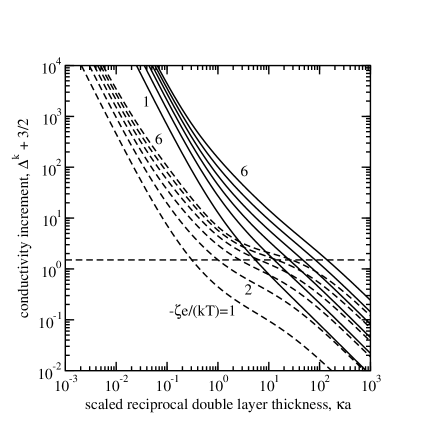
Figure 2: The conductivity increment ($3/2$ has been added to permit a logarithmically scaled ordinate) $\Delta^{k}=\Delta_{p}+\Delta_{ac}+\Delta_{nsa}$ (solid lines) as a function of the reciprocal double layer thickness $\kappa a$ for various (scaled) $\zeta$-potentials $-\zeta e/(kT)=1$, $2$, $3$, …, $6$: aqueous KNO₃ at $T=25$^∘C; $a=10$ nm; ${\ell}=1$ nm. Dashed lines are the contributions from electrostatic and concentration polarization, $\Delta_{p}$; these are practically independent of the Brinkman screening length ${\ell}$. The horizontal line at $3/2$ denotes where $\Delta^{k}=0$.

Note that the calculations presented below for the experiments with DI water as the electrolyte assume a $\zeta$-potential that is the same as in 1 mmol l^-1 KNO₃ ($\zeta=-70$ mV); the calculations also neglect the presence of dissolved CO₂. The later can be justified from the bulk conductivity being dominated by the added counterions (H₃0⁺), while the former is speculative and principally motivated by the unreasonably high $\zeta$-potentials that result when a constant surface charge is assumed. Nevertheless, when $\phi(\Delta_{ac}+\Delta_{nsa})\gg 1$, which is the case for DI water and 1 mmol l^-1 KNO₃, $K^{e}$ is influenced by $\zeta$ in the same manner as $M$. Therefore, while the value of $\zeta$ chosen to estimate $K^{e}$ influences the experimentally ascertained pore mobility $M$ [see Eqn.(19)], it affects the theoretical prediction of $M$ in the same manner, thereby yielding a similar best-fit value of ${\ell}$.

3.4 Asymptotic formulas for the pore mobility

In addition to the numerically exact solutions of the electrokinetic model, let us recall an approximate analytical solution valid for dilute composites where the $\zeta$-potential is low ($|\zeta|<kT/e$) and the double-layer thickness $\kappa^{-1}$ and Brinkman screening length ${\ell}$ are both small compared to the particle radius $a$:

$$U/(E\phi)=\frac{-9\epsilon_{s}\epsilon_{o}\zeta\kappa a({\ell}/a)^{2}}{2\eta(\kappa{\ell}+1)}\ \ (\kappa a\gg 1,{\ell}\ll a,|\zeta|<kT/e).$$ (17)

This formula confirms inferences drawn from numerical solutions of the full electrokinetic model (Hill, 2006d), and, indeed, Matos et al.’s experiments, namely that the electroosmotic flow is inversely proportional to the particle radius. However, Matos et al.’s experiments are characterized by $\kappa a<1$ with ${\ell}\sim a$. As shown below, such conditions produce an electroosmotic flow that scales with the reciprocal square of the particle radius at constant $\zeta$-potential and electric field strength.

To obtain a convenient formula for small $\kappa a$, note that the hydrodynamic force on an immobilized charged colloid vanishes with respect to the electrical force when $\kappa a\ll 1$ and $|\zeta|<kT/e$ (Hill, 2006a). Further, when $\kappa a\rightarrow 0$ and $|\zeta|<kT/e$, the electrical force approaches the bare Coulombe force $f^{E}=4\pi\epsilon_{s}\epsilon_{o}a\zeta E$. Therefore, since $f^{E}=4\pi(\eta/{\ell}^{2})C^{E}E$ (Hill, 2006c), the incremental pore mobility becomes

$$U/(E\phi)=-3\epsilon_{s}\epsilon_{o}\zeta({\ell}/a)^{2}/\eta\ \ (\kappa a\ll 1,|\zeta|<kT/e).$$ (18)

It is noteworthy that the dependence of the pore mobility on particle size is qualitatively different at high and low $\kappa a$. This is due to the relationship between the surface charge density and potential. When $\kappa a$ is large, the surface charge density is $\sim\zeta\epsilon_{s}\epsilon_{o}\kappa$, so the average mobile charge density in the hydrogel scales as $\zeta\epsilon_{s}\epsilon_{o}\kappa\phi/a$. However, when $\kappa a$ is small, the surface charge density is $\sim\zeta\epsilon_{s}\epsilon_{o}/a$, so the mobile charge density scales as $\zeta\epsilon_{s}\epsilon_{o}\phi/a^{2}$. Accordingly, balancing the electrical and Darcy drag forces gives $-E4\pi\zeta\epsilon_{s}\epsilon_{o}a\phi/[(4/3)\pi a^{3}]=(\eta/{\ell}^{2})U$, so the incremental pore mobility is $M=U/(E\phi)=-3\epsilon_{s}\epsilon_{o}\zeta({\ell}/a)^{2}/\eta$, which agrees with Eqn. (18).

Matos et al. (2006) identified the electroosmotic flow in their experiments as being inversely related to the surface area density $\phi/a$. However, their data was insufficient to ascertain a specific power-law dependence. While the theory clearly identifies the mobility as having a reciprocal square dependence with particle size at constant $\zeta$-potential when $\kappa a\ll 1$, and a reciprocal dependence when $\kappa a\gg 1$, the theoretical interpretation of the experiments is further complicated by the conductivity of the composite depending on the particle size and volume fraction. In fact, when $\kappa a\ll 1$, $K^{e}/K^{\infty}=1+O[\phi(\kappa a)^{-2}]$, so $U=\phi ME$ has a weaker dependence on particle size and volume fraction than expected if the effective conductivity were assumed constant. More importantly, and, perhaps, surprisingly, it will be demonstrated that ($i$) at very low bulk ionic strengths the electroosmotic pumping velocity $U$ at constant current density ${\cal I}=i/A$ is independent of the particle size, charge and volume fraction; and ($ii$) the effective Darcy permeability of the polymer skeleton evidently increases with decreasing average interparticle surface proximity.

Representative numerical calculations of the pore mobility are compared with the asymptotic formulas in figure 3 for inclusions with two representative radii ($a=3.5$ and $100$ nm) dispersed in an hydrogel with Brinkman screening length ${\ell}=1$ nm. In regions of the parameter space where the full model agrees with Eqn. (18) (small $\kappa a$) and (17) (large $\kappa a$ with ${\ell}\ll a$), mobilities for a different values of ${\ell}$ can be conveniently obtained by multiplying the ordinate by ${\ell}^{2}$ (measured in nm²).

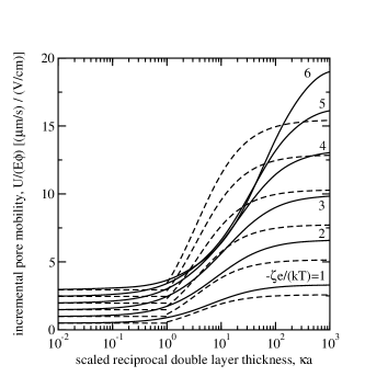
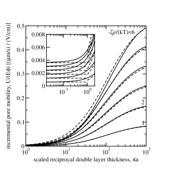
Figure 3: The incremental pore mobility $M=U/(E\phi)$ as a function of the scaled reciprocal double layer thickness $\kappa a$ for various (scaled) $\zeta$-potentials $-\zeta e/(kT)=1$, $2$, $3$, …, $6$: aqueous KNO₃ at $T=25$^∘C; $a=3.5$ (left panel) and 100 nm (right panel); ${\ell}=1.0$ nm. Solid lines are numerically exact solutions of the full electrokinetic model, and the dashed lines are approximate analytical solutions [Eqns. (17) (large $\kappa a$) and (18) (small $\kappa a$)].

4 Results

The principal methodology adopted to interpret Matos et al.’s experiments is summarized as follows. First, the measured flux enhancements and Eqn. (14) are used to determine Pe. Then, from knowledge of the electrical current ($i=3$ mA), membrane geometry ($A=1.64$ cm² and $L=1.68$ mm), particle volume fractions ($\phi=0.02$ and 0.04) and radii ($a=3.5$ and $7.5$ nm), and a theoretical calculation of the effective conductivity $K^{e}$, the incremental pore mobilities are

$$M=\mbox{Pe}D/(\phi EL)=\mbox{Pe}DK^{e}A/(\phi iL).$$ (19)

With these ‘experimentally determined’ mobilities, the electrokinetic model provides the effective hydraulic permeabilities ${\ell}^{2}$ of the hydrogel in each composite. In this manner, the theoretical interpretation, which necessitates theoretical predictions of $K^{e}$ and $M$, is evaluated by the consistency of the resulting Brinkman screening lengths ${\ell}$.

The electrokinetic transport calculations presented in table 1 were performed with unhindered ion mobilites. However, the conductivity increment and incremental pore mobility are practically independent of the ion mobilities, so it is reasonable to account for hindered ion mobilities by multiplying the unhindered bulk conductivity by a single hinderance factor. This increases the calculated electric field strength and, therefore, decreases the incremental pore mobility inferred from the experimentally measured flux enhancement. In turn, smaller best-fit values of the Brinkman screening length emerge.

The table summarizes theoretical interpretations of the five experimental conditions for which Matos et al. reported statistically averaged flux enhancements. Cases A–C and D–E, respectively, identify experiments with 1 mmol l^-1 KNO₃ and DI water. Note that DI water is approximated here as an electrolyte comprised of H₃O⁺ and OH^- ions, each with a concentration $n_{j}^{\infty}=10^{-7}$ mol l^-1, and the $\zeta$-potentials of the silica nanoparticles are taken to be $-70$ mV in 1 mmol l^-1 KNO₃ and DI water; recall, Matos et al. reported $\zeta$-potentials only for 1 mmol l^-1 KNO₃.

The upper section of the table lists quantities that are readily available from Matos et al.’s paper. In addition to the flux enhancement, $J/J_{0}$, is a length scale $a(\phi^{-1/3}-2)$ that characterizes the average distance between the inclusion surfaces. The middle section presents theoretical calculations of the polarization and added counterion and non-specific adsorption contributions to the conductivity increment (Saville, 1983). With the inclusion volume fractions and bulk electrolyte conductivity $K^{\infty}$, these provide the bulk conductivity of the composite $K^{e}$. In turn, knowledge of the current density ${\cal I}=i/A\approx 1.83$ mA cm^-2 (in the composite) provides the electric field strength $E={\cal I}/K^{e}$. Note that the conductivities of the composites saturated with DI water are comparable to those with 1 mmol l^-1 KNO₃, even though the bulk ionic strength and, hence, conductivity of the electrolyte is four orders of magnitude lower. Clearly, particle polarization and the added counterions play a very important role.

The lower section of the table presents calculations of the ‘experimentally determined’ Péclet number $\mbox{Pe}=UL/D$ and incremental pore mobility $M=U/(E\phi)$. Note that Pe may be considered a dimensionless electroosmotic pumping velocity here, since the membrane thickness $L$ and tracer diffusivity $D$ are same in all cases A–E. The table presents theoretical predictions (from numerical solutions of the full electrokinetic model) of the incremental pore mobility for composites with a Brinkman screening length ${\ell}=1$ nm. These have been used to calculate best-fit values of ${\ell}$ based on knowledge that $M$ is inversely proportional to ${\ell}^{2}$ at the prevailing values of $\kappa a<1$ (see figure 3).

Table 1: Summary of experimental data (from Matos et al., 2006) and hydrogel composite conductivity $K^{e}$, mobility $M$, and permeability ${\ell}^{2}$ calculations with unhindered ion mobilities. Note that ${\ell}_{h}$ denotes Brinkman screening lengths ascertained with hindered ion migration (see text for details): $\zeta=-70$ mV; $i=AK^{e}E=3$ mA; $A=1.64$ cm²; $L=1.68$ mm; $J/J_{0}\approx\mbox{Pe}/(1-e^{-\mbox{Pe}})$ ($\mbox{Pe}>0$).

case	$a$	$\phi$	$\kappa a$	$J/J_{0}$	$a(\phi^{-1/3}-2)$
	(nm)				(nm)
$1$ mmol l-1 KNO3 with K+ counterion
A	$3.5$	$0.02$	$0.364$	$2.36$	5.9
B	$7.5$	$0.02$	$0.780$	$1.21$	12.6
C	$7.5$	$0.04$	$0.780$	$2.21$	6.9
DI water (pH=7) with H3O+ counterion
D	$3.5$	$0.02$	$0.00364$	$1.44$	5.9
E	$7.5$	$0.02$	$0.00780$	$1.19$	12.6

case	$\Delta_{p}$	$\Delta_{ac}$	$\Delta_{nsa}$	$K^{\infty}$	$K^{e}$	$|E|$
				(mS m-1)	(mS m-1)	(V cm-1)
$1$ mmol l-1 KNO3 with K+ counterion
A	$5.08$	$89.4$	$-18.4$	$14.5$	$36.6$	$5.02$
B	$1.63$	$26.8$	$-8.55$	$14.5$	$20.2$	$9.06$
C	$1.63$	$26.8$	$-8.55$	$14.5$	$26.0$	$7.05$
DI water (pH=7) with H3O+ counterion
D	$1.70\times 10^{5}$	$7.90\times 10^{5}$	$-1.72\times 10^{5}$	$0.00549$	$86.5$	$2.12$
E	$3.74\times 10^{4}$	$1.73\times 10^{5}$	$-3.78\times 10^{4}$	$0.00549$	$18.9$	$9.70$

case	$|\mbox{Pe}|$	$|M|$(exp)	$|M|({\ell}=1.0~{}\mbox{nm})$ (theory)	${\ell}=1.0~{}\mbox{nm}\sqrt{\frac{|M|(\mbox{exp})}{|M|(\mbox{theory})}}$	${\ell}_{h}=\sqrt{0.50}{\ell}$	${\ell}_{h}=\sqrt{0.24}{\ell}$
		$\left(\frac{\mu\mbox{m}~{}\mbox{s}^{-1}}{\mbox{V}~{}\mbox{cm}^{-1}}\right)$	$\left(\frac{\mu\mbox{m}~{}\mbox{s}^{-1}}{\mbox{V}~{}\mbox{cm}^{-1}}\right)$	(nm)	(nm)	(nm)
$1$ mmol l-1 KNO3 with K+ counterion
A	$2.06$	$3.91$	$1.73$	$1.50$	$1.06$	$0.74$
B	$0.39$	$0.42$	$0.48$	$0.93$	$0.66$	$0.46$
C	$1.87$	$1.22$	$0.48$	$1.60$	$1.13$	$0.78$
DI water (pH=7) with H3O+ counterion
D	$0.78$	$3.51$	$1.34$	$1.62$	$1.14$	$0.79$
E	$0.36$	$0.35$	$0.29$	$1.09$	$0.77$	$0.53$

The scenario that emerges from these calculations is, perhaps, more complex than suggested by Matos et al.’s qualitative interpretation of the data. For example, comparing the Péclet numbers for cases A and B, where the particle size is doubled at a fixed inclusion volume fraction, suggests that $U$ scales as $a^{-2}$. While this is consistent with theoretical expectations if ${\ell}$ is a constant, doubling the particle size decreases the mobility by almost an order of magnitude. The anomaly can be reconciled by allowing ${\ell}$ to vary, but it is not clear that the resulting best-fit values of ${\ell}$ are acceptable. A similar discussion applies to the comparison of cases D and E (with DI water). Next, comparing cases B and C, where the inclusion volume fraction is doubled with a fixed particle size, the Péclet numbers indicate that $U$ more than quadruples, whereas the theory requires $U$ to double. Furthermore, the mobility triples, while the theory demands a constant mobility if ${\ell}$ is constant.

Figure 4 compares the Brinkman screening lengths ascertained from independent pressure-driven flows in thin polyacrylamide gel membranes without nano-inclusions. The two sets of data reported by White (1960) and Tokita and Tanaka (1991) are clearly very different, and it is unfortunate, perhaps, that the later authors did not reconcile these discrepancies. Nevertheless, in favor of their results is the consistency of their data with scaling theory. Accordingly, a semi-empirical fit to their data,

$${\ell}\approx 0.182c^{-0.735}\sim c^{-3/4}\ \ (\mbox{nm}),$$ (20)

gives ${\ell}\approx 0.8$ nm at the polymer concentration $c=0.13$ reported by Matos et al. (2006). This is clearly smaller than all the values of ${\ell}$ (spanning the range $0.93$–$1.62$ nm) ascertained from the theoretical interpretation of Matos et al.’s data presented in table 1.

Figure 4: The Brinkman screening length ${\ell}$ (nm) of polyacrylamide hydrogels, ascertained from pressure-driven flow experiments in thin membranes, as a function of the polymer (mass) fraction $c$: White (1960) (squares) and Tokita and Tanaka (1991) (circles). Curves are empirical fits to the data: ${\ell}=0.182c^{-0.735}$ (nm) (solid); ${\ell}=0.735\exp{(-4.36c)}$ (nm) (dashed).

Note, with a fixed value of ${\ell}=0.8$ nm, table 2 presents theoretical calculations with parameters corresponding to cases A–E in table 1. Again, all the calculations (leading to the incremental pore mobility and electrical condictivity) have been performed with unhindered electrolyte ion mobilities. The results in the upper and lower sections of the table are, respectively, with a 1 mmol l^-1 KNO₃ electrolyte (with K⁺ counterions) and DI water (with H₃O⁺ counterions).

Table 2: Theoretical expectations for Matos et al.’s experiments. Calculations with 1 mmol l^-1 KNO₃ supporting electrolyte (upper section) and DI water (lower section), both with unhindered ion mobilities: $\zeta=-70$ mV; ${\ell}=0.8$ nm; $i=AK^{e}E=3$ mA; $A=1.64$ cm²; $L=1.68$ mm; $J/J_{0}\approx\mbox{Pe}/(1-e^{-\mbox{Pe}})$ ($\mbox{Pe}>0$).

$a$	$\phi$	$\kappa a$	$\Delta_{p}$	$\Delta_{ac}$	$\Delta_{nsa}$	$K^{\infty}$	$K^{e}$	$M$	$E$	Pe	$J/J_{0}$
(nm)						(mS m-1)	(mS m-1)	$\left(\frac{\mu\mbox{m}~{}\mbox{s}^{-1}}{\mbox{V}~{}\mbox{cm}^{-1}}\right)$	(V cm-1)
$1$ mmol l-1 KNO3 with K+ counterion
$3.5$	$0.02$	$0.364$	$5.08$	$89.4$	$-18.4$	$14.5$	$36.6$	$1.11$	$5.02$	$0.57$	$1.31$
$7.5$	$0.02$	$0.780$	$1.63$	$26.8$	$-8.55$	$14.5$	$20.2$	$0.307$	$9.06$	$0.28$	$1.15$
$7.5$	$0.04$	$0.780$	$1.63$	$26.8$	$-8.55$	$14.5$	$26.0$	$0.307$	$7.05$	$0.44$	$1.24$
DI water (pH=7) with H3O+ counterion
$3.5$	$0.02$	$0.00364$	$1.70\times 10^{5}$	$7.90\times 10^{5}$	$-1.72\times 10^{5}$	$0.00549$	$86.5$	$0.860$	$2.12$	$0.19$	$1.10$
$7.5$	$0.02$	$0.00780$	$4.29\times 10^{4}$	$1.98\times 10^{5}$	$-4.34\times 10^{4}$	$0.00549$	$18.9$	$0.188$	$9.70$	$0.19$	$1.10$
$7.5$	$0.04$	$0.00780$	$4.29\times 10^{4}$	$1.98\times 10^{5}$	$-4.34\times 10^{4}$	$0.00549$	$37.8$	$0.189$	$4.85$	$0.19$	$1.10$

The calculations with a KNO₃ electrolyte indicate that the mobilities, Péclet numbers, and flux enhancements exhibit similar qualitative trends as the experiments. Howevever, the quantitative trends are poor. Note that the conductivity increments are practically the same as those presented in table 1 with ${\ell}=1$ nm. This reflects the extremely weak role of microscale convection in polarizing the inclusions, and, of course, that added counterions and non-specific adsorption are an $O(\phi)$ contribution to equilibrium.

The calculations in the lower section of the table, with DI water as the electrolyte, demonstrate that the electroosmotic flow velocity, as indicated by Pe or $J/J_{0}$, is practically independent of the particle size and volume fraction at sufficiently low bulk ionic strengths. If the discrepancy between the electroosmotic flow velocity $U=\mbox{Pe}D/L\approx 37$ nm s^-1 and the experimentaly determined value $U\approx 74$ nm s^-1 for DI water (when $a(\phi^{-1/3}-2)\approx 11.8$) can be attributed to the neglect of hindered ion migration, which leads to an incorrect estimate of the bulk conductivity $K^{\infty}$, then the effective electrolyte ion hinderance factor is suggested to be about $37/74\approx 0.50$. This is in reasonable agreement with independent measurements of the hindered diffusion coefficients of KCl and D₂O (and two larger molecules) in polyacrylamide hydrogels. In particular, at the bulk polymer concentration used in Matos et al.’s experiments ($c\approx 0.13$), White and Dorion (1961) measured diffusion coefficients of KCl and D₂O that are factors of $1.2/1.8\approx 0.67$ and $1.2/2.2\approx 0.55$ smaller than their respective unhindered values.

Accordingly, if it is assumed that the electrical conductivity of the membranes is indeed reduced by a factor of 0.50, and, furthermore, the mobilities of all electrolyte ions are reduced by the same factor, then the incremental pore mobilities $M$ inferred from Matos et al.’s experiments should be a factor 0.50 smaller than the values listed in table 1. Moreover, the best-fit Brinkman screening lengths ${\ell}$ in the table should be reduced by a factor $\sqrt{0.50}\approx 0.71$. These values are denoted ${\ell}_{h}=\sqrt{0.50}{\ell}$ in the lower section of table 1. It is noteworthy that their range $0.66$–$1.14$ nm is much more representative of the values expected from the pressure-driven flows of White (1960) and Tokita and Tanaka (1991).

Knowledge of the electrical conductivity of the electrolyte-saturated hydrogel would provide an independent quantitative measure of the influence that the polymer has on electrolyte ion mobilities while under the influence of an electric field. Unfortunately, the electrical conductiviy of the hydrogels in Matos et al.’s experiments is unknown. However, data in Matos’s thesis (fig. 4.29 Matos, 2006) indicates that the voltage drop across the entire cell (i.e., between the electrodes) when $i=3$ mA is about $12$ V when gels without inclusions are saturated with 1 mmol l^-1KNO₃. If this voltage is assumed to reflect only the combined electrical resistances of the membrane and electrolyte sandwiched between the electrodes, then the conductivity of the membrane is

$$K^{e}=K^{\infty}/[K^{\infty}A\Delta/(iL)-(L^{\prime}/L)(A/A^{\prime})].$$ (21)

Here, $\Delta\approx 12$ V is the total potential drop, $K^{\infty}\approx 14.5$ mS m^-1 is the conductivity of 1 mmol l^-1KNO₃ electrolyte (from knowledge of the limiting conductances of $K^{+}$ and NO${}_{3}^{-}$), $L^{\prime}=6-1.68=4.32$ mm is twice the distance between the membrane and one electrode, and $A^{\prime}\approx 2.84$ cm² is the clear cross-sectional area between the membrane and electrodes. It follows that $K^{e}\approx K^{\infty}/(5.66-1.56)\approx 0.24K^{\infty}$. While this indicates that the polymer significantly hinders ion migration, the calculation is likely to over-estimate the hindrance, because it neglects the (unknown) potential drop due to electrochemical reactions.

Nevertheless, with a hinderance factor of $0.24$ adoped to provide a lower-bound on the membrane electrical conductivity, the corresponding Brinkman screening lengths, denoted ${\ell}_{h}=\sqrt{0.24}{\ell}$ in the lower section of table 1, are a factor $\sqrt{0.24}\approx 0.49$ smaller than the best-fit values ascertained with unhindered ion mobilities. The range ${\ell}_{h}=0.53$–$0.79$ nm is representative of the values expected from the pressure-driven flows of White (1960) and Tokita and Tanaka (1991), but, as highlighted below, such a favorable comparision may be misleading.

The analysis summarized in table 1 has led to an upper range ${\ell}\approx 0.9$–1.60 nm ascertained with unhindered ion mobilities, and a lower range ${\ell}_{h}\approx 0.53$–$0.79$ nm ascertained using a lower-bound estimate of hindered ion mobilities. Note that fluctuations within each range correspond to unreasonably large fluctuations in the bulk polymer density, and such fluctuations cannot be reconciled by osmotic swelling. It therefore remains to elucidate these significant variations in gel permeability.

5 Discussion

One clue to resolving the apparent shortcomings is to recognize that two distinctly different values of the best-fit Brinkman screening lengths emerge from the experiments. Considering, for example, the values ascertained with unhindered ion mobilities, cases B and E yield values of ${\ell}$ close to 1 nm, whereas cases A, C and D yield values close to 1.5 nm. These differences do not correlate with the electrolyte, particle size or volume fraction alone. However, there is strong correlation with a length scale that characterizes the average distance between closest neighbors in a uniform random dispersion. Letting the characteristic center-to-center distance be $a\phi^{-1/3}$, the distance between the surfaces is $a(\phi^{-1/3}-2)$. This measure is listed in the last column of the upper section of table 1, and its relationship to the effective permeability is plotted in figure 5.

Figure 5: The effective Brinkman screening length ${\ell}^{e}$ as a function of the average distance between the surfaces of nearest neighbor inclusions in random dispersions $a(\phi^{-1/3}-2)$: upper-bound estimates based on theoretical interpretation of experiments with unhindered ion mobilities (open symbols); lower-bound estimates achieved with a lower-bound estimate of hydrogel electrical conductivity (filled symbols). See text for details. Circles and squares denote, respectively, cases A–C with 1 mmol l^-1KNO₃ electrolyte, and cases D and E with DI water (see table 1). The solid lines are empirical best-fit (quadratic) decays: ${\ell}^{e}={\ell}[1+47.3/\{(\phi^{-1/3}-2)a/{\ell}\}^{2}]$ with ${\ell}=0.83$ nm (upper curve); ${\ell}^{e}={\ell}[1+184/\{(\phi^{-1/3}-2)a/{\ell}\}^{2}]$ with ${\ell}=0.42$ nm (lower curve). Dashed lines indicate the values of ${\ell}$ expected from pressure-driven flows in polyacrylamide gels with a polymer concentration $c\approx 0.13$: ${\ell}\approx 0.8$ nm (Tokita and Tanaka, 1991) (upper line); ${\ell}\approx 0.4$ nm (White, 1960) (lower line).

Recall, the best-fit values of ${\ell}$, ascertained without hindered ion mobilities influencing the membrane electrical conductivity, provide an upper-bound on the effective gel permeability (open symbols). Furthermore, the lower-bound on the electrical conductivity, established above from the voltage-current relationship for the cell, provides a lower-bound-estimate of the gel permeability (filled symbols). As demonstrated in the figure 5, these upper- and lower-bounds approach values expected from independent pressure-driven flow experiments in homogeneous (i.e., without inclusions) polyacrylamide gels (Tokita and Tanaka, 1991; White, 1960). Moreover, the approach occurs as the separation $a(\phi^{-1/3}-2)$ becomes large compared to ${\ell}$.

This quantitative analysis supports Matos et al.’s suggestion that particle interactions play a necessary role in endowing the composites with a significant electroosmotic pumping capacity. Nevertheless, the physical origin of such interactions and, indeed, their quantitative influence on the electroosmotic pumping capacity and bulk conductivity remain unknown.

Matos et al. suggested that electroosmotic flow creates pathways that somehow link particles in close proximity, as expected in a percolating network. However, their neutron scattering data did not reflect fractal-like correlations. Another possibility is that polymer structure (e.g., partial chain orientation and/or cross-linking density) is altered near the particle surfaces, producing shells of hydrogel that are much more electrically conductive (i.e., with higher ion permeabilities) and hydrodynamically permeable than in the bulk. Swelling after the synthesis could also generate shells of void space.

It is tempting to draw upon Matos et al.’s data with $a=3.5$ nm and $\phi=0.005$, 0.01 and 0.2 (as seen in fig. 8 of Matos et al., 2006) to help elucidate the role of particle volume fraction and size. However, it is evident from these single experiments, and the averaged data (used exclusively above), that there are significant statistical fluctuations from one experiment to another. For example, the flux enhancements from the experiments presented in figures 1 and 8 of Matos et al.’s paper with DI water (with $a=3.5$ nm and $\phi=0.02$) are, respectively, $\approx 1.58$ and 1.63, whereas the flux enhancement from repeated measurements under the same conditions was reported as $1.44\pm 0.01$ (as adopted in table 1 above). It is also difficult to draw firm conclusions from the experiments with DI water, since the $\zeta$-potentials are unknown, further hampering theoretical estimates of the bulk conductivity and incremental pore mobility.

Finally, note that silica nanoinclusions have been demonstrated to enhance the permeability of glassy polymeric matrices to gases (Merkel et al., 2002). This unexpected behavior is attributed to an overall increase in the free volume of the polymer. Moreover, recent theoretical studies show that the increase in free volume is localized to the particle-polymer interface (Hill, 2006b). The interpretation of Matos et al.’s experiments summarized in figure 5 suggests that a similar influence prevails when silica nanoparticles are immobilized in swollen water-saturated polymer networks.

6 Summary

The full electrokinetic transport model proposed by Hill (2006d) was used to interpret recent experiments where Matos et al. (2006) immobilized silica nanospheres in an uncharged polayacrylamide hydrogel matrices and applied an electric field to electroosmotically enhance the otherwise a purely diffusive flux of an uncharged tracer across the composite membrane.

Convenient simplifications of the full model, leading to simple closed-form formulas, were derived for the limit where the bulk ionic strength is low and the inclusion radius is small; these complement earlier analytical solutions for situations where the Debye and Brinkman screening lengths are small compared to the particle radius. The analytical results were demonstrated to yield accurate approximations of the incremental pore mobility from numerically exact solutions of the full electrokinetic model. Figure 3 identifies practical bounds on the parameter space where these convenient approximations are accurate.

A simple (quasi-steady) convective-diffusion model for the tracer flux was derived to quantitatively interpret the flux-enhancement diagnostic reported by Matos et al. The general solution depends on the (changing) concentration of tracer in the source and sink reservoirs, but it was assumed here that the concentration in the sink was small enough to permit an approximation that relates the scaled electroosmotic flow velocity ($\mbox{Pe}=UL/D>0$) directly to the flux enhancement $J/J_{0}>1$.

Several approaches were taken to compare the theory and experiments. One involved selecting the Brinkman screening length of the polymer skeleton as a fitting parameter and using the experiments and theory to establish values that yield ‘correct’ flux enhancements. With unhindered electrolyte migration, the effective Brinkman screening length of the hydrogels was found to span the range $0.93$–$1.63$ nm, depending, foremost, on the average particle separation, as measured by $a(\phi^{-1/3}-2)$. Evidently, as the particle separation diverges, the effective Brinkman screening length approaches a value ($\approx 0.8$ nm) that is expected from independent pressure-driven flow experiments by Tokita and Tanaka (1991). On the other hand, allowing for hindered electrolyte ion migration, a lower-bound-estimate of the efffective Brinkman screening length gives a range $0.46$–$0.79$ nm. Similarly, as the particle separation diverges, the effective Brinkman screening length approaches a value ($\approx 0.4$ nm) that is expected from independent pressure-driven flow experiments by White (1960).

Several means of reconciling the apparent differences between theory and experiment were proposed, all of which require more extensive and complete experimental investigation to draw firm conclusions. Firstly, this analysis supports Matos et al.’s suggestion that particle interactions, which are neglected entirely in the present theory (due to the small inclusion volume fraction), significantly increase the electroosmotic pumping capacity of the composites. A model to quantify the influence of such interactions has not been pursued, and it is not clear that the enhanced permeability arises from particle-particle or particle-polymer interactions, or, perhaps, a combination of both.

While the electroosmotic pumping capacity of a composite is independent of the bulk electrical conductivity, when the electric field driving the flow is known, in practice it is the electrical current that is known accurately. This necessitates an accurate experimental determination of the bulk conductivity to complement a satisfactory theoretical interpretation of experiments, and thus permit an accurate prediction of the pumping capacity as a function of current density.

Clearly, it would be advantageous if future experimental efforts reported the conductivity of hydrogels with and without inclusions, preferentially when uniformly saturated with well-characterized electrolytes, including DI water. Such diagnostics should be performed using a high-frequency electric field while the membrane is in its steady or quasi-steady state, i.e., when subjected to a steady electric field. Note, however, that care must be taken to separate the influences of the bulk and near-electrode regions (Hollingsworth and Saville, 2003).

Supported by the Natural Sciences and Engineering Research Council of Canada (NSERC), through grant number 204542, and the Canada Research Chairs program (Tier II).

References

- Brinkman (1947) Brinkman, H. C., 1947. A calculation of the viscous force exerted by a flowing fluid on a dense swarm of particles. Appl. Sci. Res. A 1, 27–34.
- Chang et al. (1995) Chang, Y.-H. D., Grodzinsky, A. J., Wang, D. I. C., 1995. Augmentation of mass transfer through electrical means for hydrogel-entrapped Escherichia coli cultivation. Biotechnology and Bioengineering 48, 149–157.
- Hill (2006a) Hill, R. J., 2006a. Electric-field-induced force exerted on a charged spherical colloid embedded in an electrolyte-saturated Brinkman medium. Phys. Fluids 18, 043103.
- Hill (2006b) Hill, R. J., 2006b. Reverse-slective diffusion in nanocomposite membranes. Phys. Rev. Lett. 96 (21), 216001.
- Hill (2006c) Hill, R. J., 2006c. Transport in polymer-gel composites: Response to a bulk concentration gradient. J. Chem. Phys. 124, 014901.
- Hill (2006d) Hill, R. J., 2006d. Transport in polymer-gel composites: theoretical methodology and response to an electric field. J. Fluid Mech. 551, 405–433.
- Hill et al. (2003) Hill, R. J., Saville, D. A., Russel, W. B., 2003. Polarizability and complex conductivity of dilute suspensions of spherical colloidal particles with uncharged (neutral) polymer coatings. J. Colloid Interface Sci. 268, 230–245.
- Hollingsworth and Saville (2003) Hollingsworth, A. D., Saville, D. A., 2003. A broad frequency range dielectric spectrometer for colloidal suspensions: cell design, calibration, and validation. J. Colloid Interface Sci. 257 (1), 65–76.
- Matos (2006) Matos, M., April 2006. Electroosmotic mass transport control in polyacrylamide gels via embedded silica nanoparticles. Ph.D. thesis, Carnegie Mellon University, Pittsburgh, Pennsylvania 15213.
- Matos et al. (2006) Matos, M. A., White, L. R., Tilton, R. D., 2006. Electroosmotically enhanced mass transfer through polyacrylamide gels. J. Colloid Interface Sci. 300, 429–436.
- Merkel et al. (2002) Merkel, T. C., Freeman, B. D., Spontak, R. J., He, Z., Pinnau, I., Meakin, P., Hill, A. J., 2002. Ultrapermeable, reverse-selective nanocomposite membranes. Science 296, 519–522.
- Saville (1983) Saville, D. A., 1983. The electrical conductivity of suspensions of charged particles in ionic solutions: The roles of added counterions and nonspecific adsorption. J. Colloid Interface. Sci. 91 (1), 34–50.
- Tokita and Tanaka (1991) Tokita, M., Tanaka, T., 1991. Friction coefficient of polymer networks of gels. J. Chem. Phys. 95 (6), 5613–4619.
- White (1960) White, M. L., 1960. The permeability of an acrylamide polymer gel. J. Phys. Chem. 64 (10), 1563–1565.
- White and Dorion (1961) White, M. L., Dorion, G. H., 1961. Diffusion in a crosslinked acrylamide polymer gel. J. Polymer Sci. 55, 731–740.
- Yao et al. (2003) Yao, S., Hertzog, D. E., Mikkelsen, J. C. J., Santiago, J. G., 2003. Porous glass electroosmotic pumps: design and experiments. J. Colloid Interface Sci. 268, 143–153.
- Yao and Santiago (2003) Yao, S., Santiago, J. G., 2003. Porous glass electroosmotic pumps: theory. J. Colloid Interface Sci. 268, 133–142.
- Yukawa et al. (1976) Yukawa, H., Yoshida, H., Kobayashi, K., Hakoda, M., 1976. Electroosmotic dewatering of sludge under condition of constant voltage. J. Chem. Eng. Japan 9 (5), 402–407.