Noise effects in extended chaotic system: study on the Lorenz’96 model

Abstract

We investigate the effects of a time-correlated noise on an extended chaotic system. The chosen model is the Lorenz’96, a kind of toy model used for climate studies. The system is subjected to both temporal and spatiotemporal perturbations. Through the analysis of the system ${}^{\prime}s$ time evolution and its time correlations, we have obtained numerical evidence for two stochastic resonance-like behaviors. Such behavior is seen when a generalized signal-to-noise ratio function are depicted as a function of the external noise intensity or as function of the system size. The underlying mechanism seems to be associated to a noise-induced chaos reduction. The possible relevance of those findings for an optimal climate prediction are discussed, using an analysis of the noise effects on the evolution of finite perturbations and errors.

I Introduction

It is well known that noise and chaos represent, respectively, two kinds of essentially different phenomena. The former is induced by genuine stochastic sources, while the randomness of the later is pseudo and is deterministic in its origin. The spatiotemporal chaos is intrinsically irregular in both space and time and represents a prototype of deterministic randomness. It is interesting to see what would come about as a result of the interaction between these two irregularities that are essentially distinct.

As the influence of noises on low-dimensional dynamics systems has been studied extensively RMP ; mangwio , much research interest has nowadays shifted to spatially extended system, a situation that is apparently much more complicated sancho .

In the spatially extended situations, the way in which the noise takes effect is not obvious and the deterministic description usually cannot give the right results. It is known that noise-induced phenomena have come about as a consequence of nonlinear interaction between the noise and the deterministic dynamics. The spatiotemporal stochastic resonance are believed to have potential importance, for instance, in the area of signal and image processing, pattern formation, social and economical as well as climate dynamics RMP ; extend2 .

Here we consider a fully study on the Lorenz’96 model, driven by two kinds of perturbations, a deterministic perturbation given by the own chaotic behavior of the model and a stochastic one which we have assumed as an effective way of including a more realistic evolution. The relevance of this model rest on the fact that it represents a simple but still realistic description of some physical properties of global atmospheric models.

Manifestations of noise on other characteristics of spatiotemporal chaos such as Lyapunov exponents and dimensions have not been considered. The results presented here provided a first step in order to explore the possibilities of complex dynamics coming out from the interaction between chaos and noise clearly. Further investigation along this line is desirable.

This work is organized as follows: in section II we describe the Lorenz’96 model assuming that its evolution is governed by both a deterministic and a stochastic processes. In section III we present and discuss numerical simulations of the Lorenz’96 equation, describing qualitatively the interaction of the real noise and the deterministic noise on the time evolution of the system. In section IV we discuss the important problem of the perturbations and errors in the Lorenz’96 evolution. Finally in section V we present the conclusions of our work as well as possible implications and the relevance of this study on the actual climate evolution.

II The Lorenz’96 model

The equations corresponding to the Lorenz’96 model are

$$\dot{x}_{j}(t)=-x_{j-1}(x_{j-2}-x_{j+1})-x_{j}+F,$$ (1)

where $\dot{x}_{j}$ indicates the time derivative of $x_{j}$

$$F_{j}(t)=F_{med}+\Psi_{j}(t),$$ (2)

with $\Psi_{j}(t)$ a dichotomic process. That is, $\Psi_{j}(t)$ adopts the values $\pm\Delta$ with a transition rate $\gamma$: each state changes according to the waiting time distribution $\varphi_{i}(t)\sim e^{-\gamma t}$. The noise intensity for this process is defined through $\xi=\frac{\Delta^{2}}{2\gamma}$. In this work we have supposed that the system is subjected to a spatiotemporal perturbation as well as a temporal one. The first perturbation is achieved when $F$ depends on both $j$ and $t$ variables, meanwhile for temporal perturbation the $F$ function only depends on $t$. In order to simulate a scalar meteorological quantity extended around a latitude circle, we consider periodic boundary conditions $x_{0}=x_{N}$, $x_{-1}=x_{N-1}$.

As indicated before, the Lorenz’96 model has been heuristically formulated as the simplest way to take into account certain properties of global atmospheric models. The terms included in the equation intend to simulate advection, dissipation, and forcing respectively. In contrast with other toy models used in the analysis of extended chaotic systems and based on coupled map lattices, the Lorenz’96 model exhibits extended chaos when the $F$ parameter exceeds a determinate threshold value ($F>9/8$) with a spatial structure in the form of moving waves. The length of these waves is close to $5$ spatial units. It is worth noting that the system has scaled variables with unit coefficients, hence the time unit is the dissipative decay time. In addition we adjust the value of the parameter $F$ to give a reasonable signal to noise ratio (Lorenz considered $F=8$), so the model could be most adequate to perform basic studies of predictability.

II.1 System Response

As a measure of the SR system’s response we have used the signal-to-noise ratio (SNR) RMP . To obtain the SNR we need to previously evaluate $S(\omega)$, the power spectral density (psd), defined as the Fourier transform of the correlation function vK ; Gar

$$S(\omega)=\int_{-\infty}^{\infty}e^{i\omega\tau}\langle x_{j}(0)x_{j}(\tau)\rangle\,d\tau,$$ (3)

where $\langle\,\,\,\rangle$ indicates the average over realizations. As we have periodic boundary conditions simulating a closed system, $\langle x_{j}(0)x_{j}(\tau)\rangle$ has a homogeneous spatial behavior. Hence, it is enough to analyze the response in a single site.

We consider two forms of SNR. In one hand the usual SNR measure at the resonant frequency $\omega_{o}$ (that is, in fact, at the frequency associated to the highest peak in $S(\omega)$) is

$$SNR=\frac{\int^{\omega_{o}+\sigma}_{\omega_{o}-\sigma}d\varpi S(\varpi)}{\int^{\omega_{o}+\sigma}_{\omega_{o}-\sigma}d\varpi S_{back}(\varpi)},$$ (4)

where $2\sigma$ is a very small range around the resonant frequency $\omega_{o}$, and $S_{back}(\omega)$ corresponds to the background psd. On the other hand we consider a global form of the SNR ($SNR_{glob}$) defined through

$$SNR_{glob}=\frac{\int^{\omega_{max}}_{\omega_{min}}d\omega S(\omega)}{\int^{\omega_{max}}_{\omega_{min}}d\omega S_{back}(\omega)},$$ (5)

where $\omega_{min}$ and $\omega_{max}$ define the frequency range where $S(\omega)$ has a reach peak structure (with several resonant frequencies).

III Stochastic resonance-like effects

III.1 System Time Evolution

In this section we present numerical simulations of a Lorenz ’96 system subjected to both temporal and spatiotemporal noise perturbations. The typical numbers we have used in our simulations are: averages over $10^{3}$ histories, and $\sim 10^{4}$ simulation time steps (within the stationary regime, see later).

We have analyzed the typical behavior of trajectories as $x_{1}(t)-x_{med-T}$, where $x_{med-T}$ is the time average. When the Lorenz ’96 system evolves without external noise ($F_{j}(t)$ is constant), the time evolution shows a random-like behavior. As can be seen in Fig. 1-a where we describe the $|x_{1}-x_{1MedT}|$, the main feature is that the amplitude of the oscillator is almost constant over all the time. If the system is subject to a true random force, described like in Eq.[1] as shown in Fig. 1 - b, then the temporal oscillator response decays, that is the interaction between the intrinsic evolution and the external noise produces dissipation on the system. Hence the time evolution of the system consists of a transitory regime and a stationary one.

We have assumed that this decay can be adjust by an exponential law ($|x_{1}-x_{1\,\ Med\,\ T}|\sim\exp(-\lambda t)$). Figures 2-a depicts the $\lambda$ dependence on the transition rate $\gamma$ for a spatiotemporal evolution. The figure shows the weak dependence of $\lambda$ on $\gamma$ for two $F_{Med}$ parameters. In one hand the temporal decay parameter depends on the $F_{med}$ parameter as can be seen in the insert of the Fig. 2-a. On the other hand there exists a clear dependence of $\lambda$ when the system is subject to only temporal perturbation (see Fig. 2 - b). Two regions can be observed, firstly a quasi linear grow for a low rate transitions and a saturation regime for large $\gamma$. It is worth remarking here that this saturation regime is not the same than that for a spatiotemporal perturbation. The indicated time decay is important as we are interested in studying the noise effects on the stationary regime.

Figure 1: System parameters $N=128$, $F_{Med}=5$. (a) Time evolution without noise. (b) Time evolution with noise $\Delta=1$, $\gamma=0.05$.

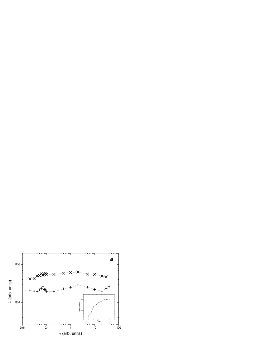
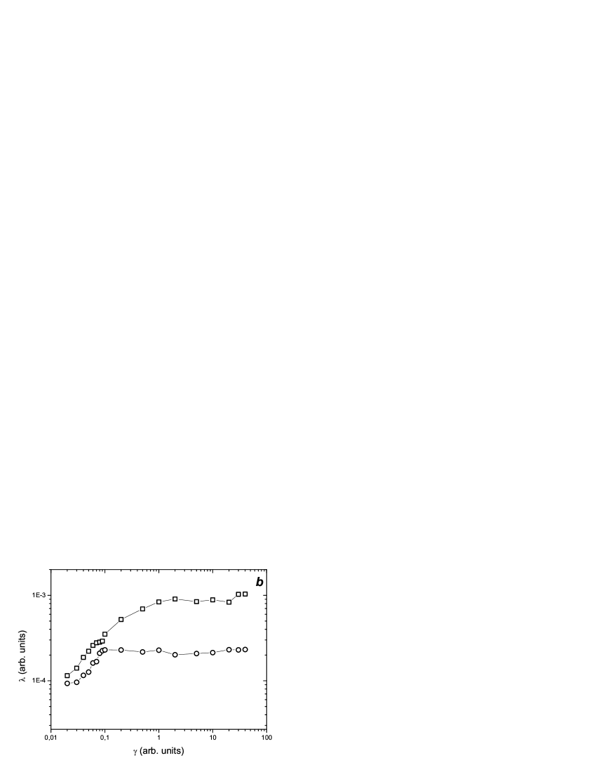
Figure 2: (a) Spatiotemporal evolution. Decay rate vs. transition rate $\times F_{Med}=6$, $+F_{Med}=5$, $N=64$ Insert: Decay rate vs. $F_{Med}$ (b) Temporal evolution. $F_{Med}=6$ circles, $F_{Med}=5$ squares.

III.2 Resonant-like behavior

Figure 3-a shows the power spectrum density (psd) for two cases, the Lorenz’96 model without noise (continuous line) and when subject to a dichotomic noise (dash line). From the figure it is apparent that the simultaneous action of both deterministic and stochastic noises induces a background reduction. The consequence of this effect can be appreciated in the Fig. 3 - b where it is possible to anticipate, and identify, the existence of a resonance-like behavior when the global signal to noise ($SNR_{Global}$) is depicted as a function of the noise intensity ($\Delta$). Indeed the response for $F_{Med}=5$ is better than for $F_{Med}=6$. The insert of the figure shows the $SNR_{Global}$ response as a function of the $F_{Med}$ parameter for two different noise intensities. We can see that the response is high for low values of $F_{Med}$ (low developed chaos) and that is almost constant for large values of $F_{Med}$ (well developed chaos).

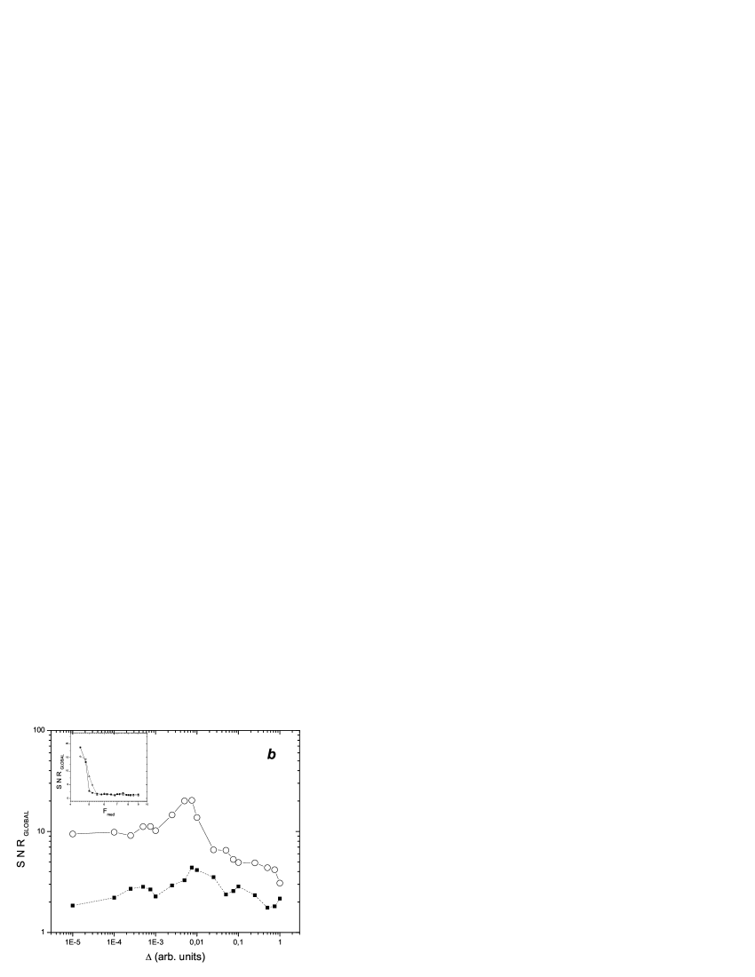
Figure 3: (a) Power spectral density. Solid line: Lorenz $96$ without noise. Dash line: Lorenz $96$ evolution with $\Delta=0.1$, $F_{Med}=5$, $N=128$. (b) Signal to noise ratio for $F_{Med}=5$ circles, $F_{Med}=6$ squares. Insert: signal to noise ratio as a function of $F_{Med}$.

We have also studied the response dependence on the transition rate $\gamma$. Figure 4-a (spatiotemporal noise for two $F_{Med}$) and Fig. 4-b (spatiotemporal and temporal noise) show these behaviors. Figure 4-a shows that there is a weak dependence of the $SNR_{Global}$ for low values of $\gamma$. On one hand, in general for the spatiotemporal noise, the $SNR_{Global}$ is constant and a weak dependence with the $F_{Med}$ is apparent. On the other hand, there exists a dependence of the $SNR_{Global}$ when temporal noise is applied. Again, we can distinguish two regimes: a first linear one for low transition rate ($\gamma<0.5$) and a quasi constant regime for $\gamma>0.5$. The figure also shows that the SNR response is different when the system is subject to temporal or spatiotemporal perturbations. It is important to remark that for large $\gamma$ the temporal SNR is larger than for spatiotemporal perturbations.

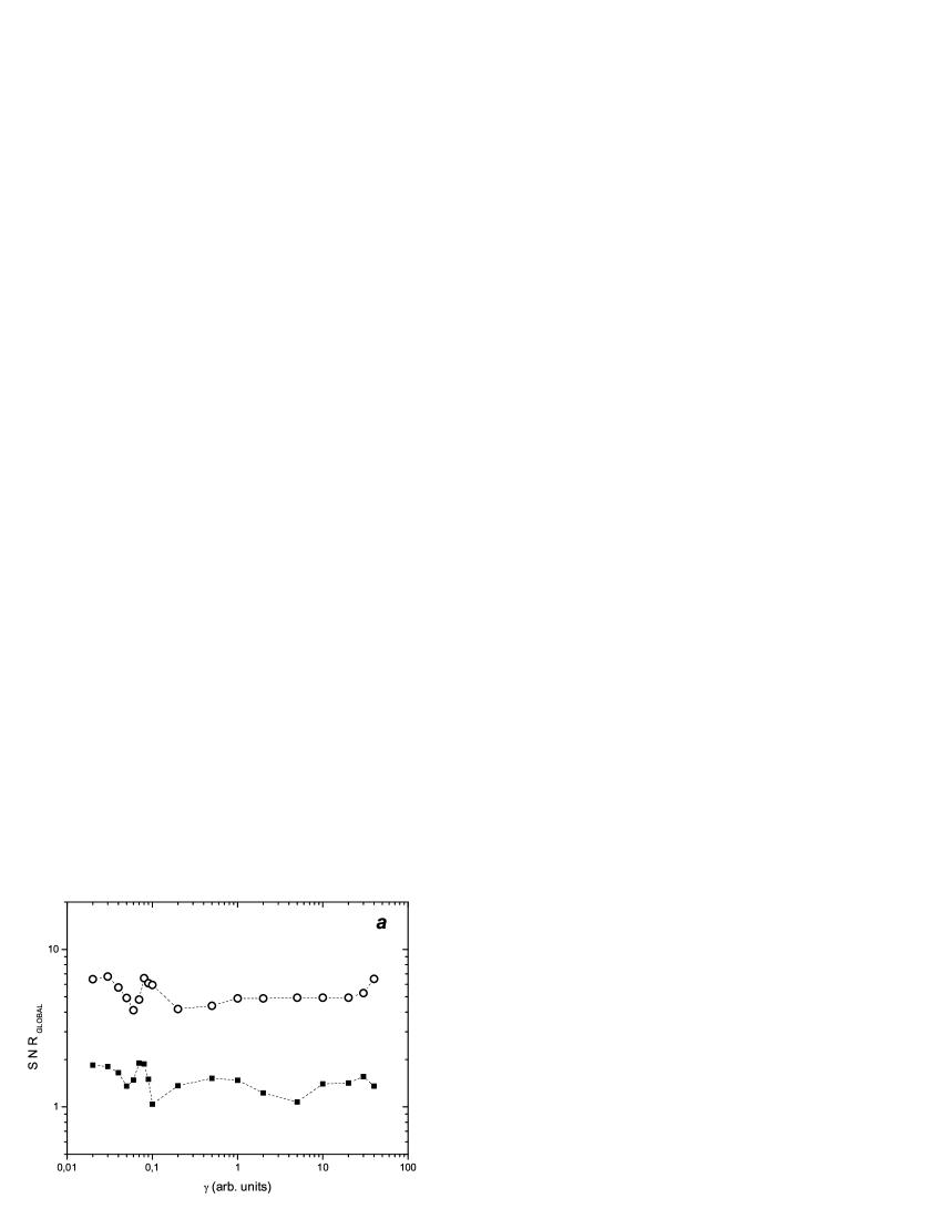
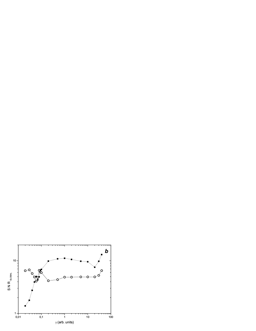
Figure 4: (a) Spatiotemporal evolution. Signal to noise ratio as a function of the transition rate. $F_{Med}=5$ circles, $F_{Med}=6$ squares. (b)Spatiotemporal (circle) and temporal (square) SNR for a $N=64$ system, with $\Delta=0.1$.

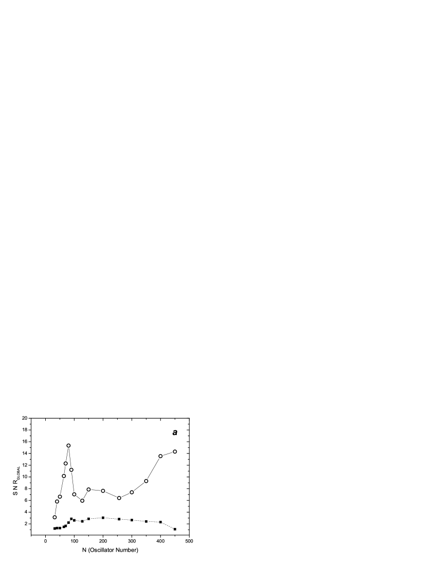
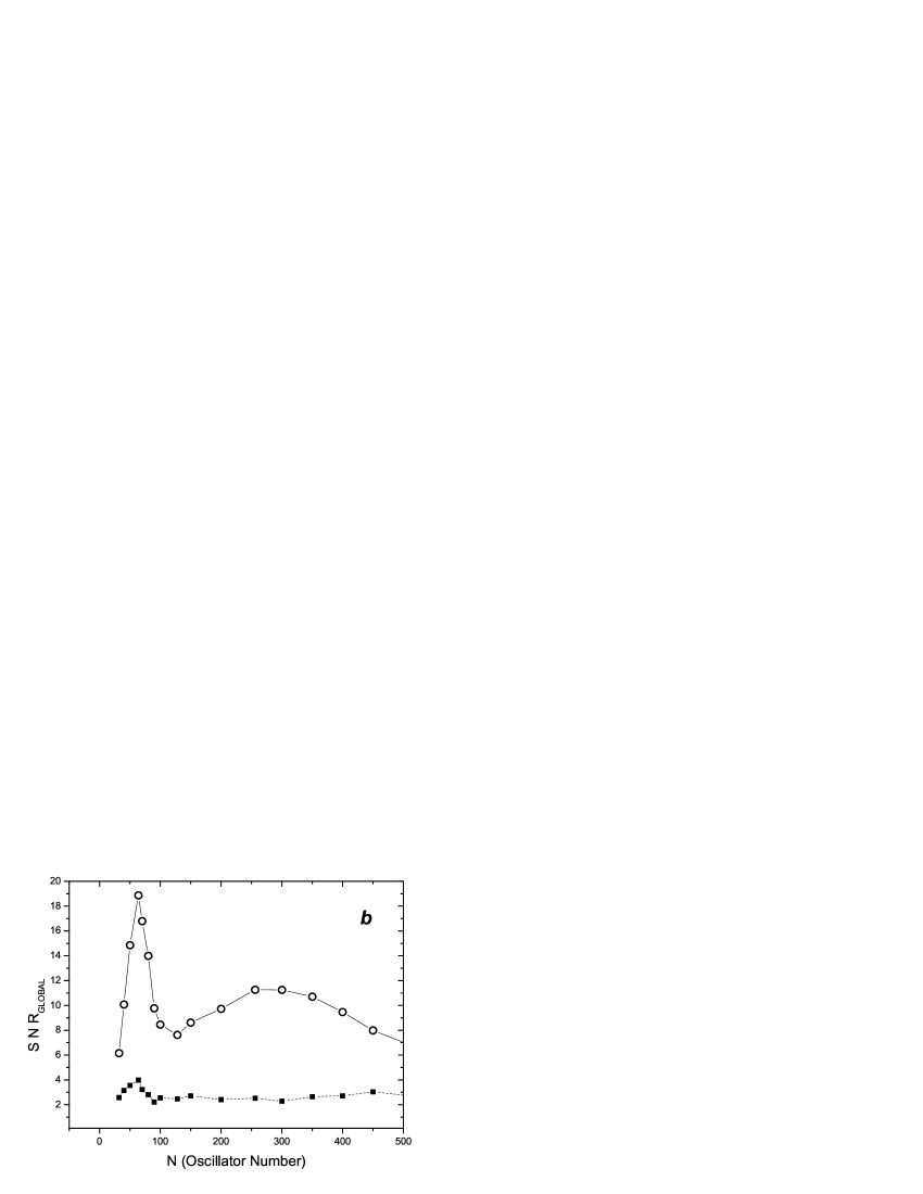
Figure 5: Signal to noise ratio for (a)spatiotemporal evolution . (b) Temporal evolution. Open circle correspond to $F_{Med}=5$, square to $F_{Med}=6$.

Finally in Figs. 5-a and 5-b we show the results obtained for the behavior of the global SNR as a function of the system size. The figures show a resonant-like behavior for a size around $80$ in the low developed chaos case, meanwhile this phenomenon is weaker when the chaos is more developed. This behavior is analogous to the so called system size stochastic resonance sssr

At this point it is worth to comment on the similarities of the SR-like phenomena found here and the so called internal signal SR int . Previous studies have shown that in some systems having an internal typical frequency, SR can occur not only at the frequency of an external driving signal, but also at the frequency corresponding to the internal periodic behavior int . Regarding the present mechanism of SR, what we can indeed remark is that the increase in the SNR is related not to a reinforcement of the peak high respect to the noisy background at a given frequency, but with a reduction of the pseudo (or deterministic) noisy background when turning on the real noise. That is, the interplay between “real” noise and “deterministic” noise conforms a kind of noise-induced chaos reduction. Figure 3a shows, for fixed values of $F$ and $\gamma$, the behavior of $S(\omega)$ in both cases: with ($\Delta\neq 0$) and without noise ($\Delta=0$). The above indicated reduction trend, as the real noise is turned on, is apparent.

The above indicated trend seems to be also responsable of the behavior observed in Fig. 4a, as $\gamma$ also enters into de definition of the noise intensity. From Fig. 4b it becomes clear that the spatial-temporal noise has a stronger influence than the temporal one on the system response.

IV Finite perturbations and errors

The exponential growth of small initial perturbations is the main effect of chaos and the origin of the lack of prediction in deterministic dynamical systems. This growth is not homogeneous but localized in some unstable directions that are fix in low dimensional cases (usual localization) and moving in the case of extended chaos (dynamic localization) PiK . Moreover, in a real system perturbations do not grow indefinitely but saturate by the action of non-linearities. Hence, in real situations we must deal with finite perturbations FinPert that, for small enough initial perturbations, develop in two regimes, the infinitesimal one characterized by a exponential growth localized in some directions and the above mentioned non-linear regime in which saturation by non-linear effects destroy the exponential growth as well as the gained localization Patterns .

An important problem in predictability analysis is just the characterization and quantification of both the exponential growth and the degree of localization. The Lyapunov theory of perturbation analysis has been a traditional tool to solve particulary the first part of this problem related with the exponential growth. In the case of spatial chaos there is a recent theory that accounts for both parts in a very convenient form. It is based on mapping perturbations in rough surfaces trough the application of a logarithmic transformation (the Hopf-Cole transformation). The use of this mapping simplifies the analysis of perturbations due to several reasons; the statistics in the mapped space is Gaussian (or Poissonian, etc..) instead of being log-normal (log-Poisson, etc..) Predict . Moreover, the growth of rough interfaces is supported by a well established theory with well defined time and length scales that are connected by scaling laws DynScal , and finally there are universal types of growth which offers very good forms of characterization. As we show in the next sections the use of this mapping provides us with a powerful tool to analyze the interplay of chaos and noise in a spatial chaotic system.

IV.1 The Mean-Variance of Logarithms diagram for perturbations and errors

Finite perturbations from the original Eq.[1] are obtained by evolving with exactly the same equation (noise included) a perturbed initial condition $x_{i}^{\prime}(0)=x_{i}(0)+\delta x_{i}(0)$. At a longer time finite perturbations are then given by the difference $\delta x_{i}(t)=x_{i}(t)-x_{i}^{\prime}(t)$. We refer to it as a perturbation because only changes in the initial conditions are considered. In this aspect the noise, which is the same in both realizations, acts as deterministic and can be considered as a parametrization of small scale phenomena. On the other hand the definition of finite error is the same $\epsilon_{i}(t)=x_{i}(t)-x_{i}^{\prime}(t)$ but now the evolution of both the control system ($x_{i}(t)$) and the perturbed one ($x_{i}^{\prime}(t)$) are obtained with different realizations of noise.

In the infinitesimal regime of finite fluctuations one can write an equation for perturbations just linearizing around the control trajectory, that reads

$$\frac{d\delta x_{j}}{dt}=x_{j-1}\delta x_{j+1}-x_{j-1}\delta x_{j-2}+(x_{j+1}-x_{j-2})\delta x_{j-1}-\delta x_{j},$$ (6)

while for for errors we have

$$\frac{d\delta X_{j}}{dt}=X_{j-1}\delta X_{j+1}-X_{j-1}\delta X_{j-2}+(X_{j+1}-X_{j-2})\delta X_{j-1}-\delta X_{j}+\psi_{i}(t),$$ (7)

that is the same equation, but including an additive noise term $\psi_{i}(t)=F_{i}(t)-F_{i}^{\prime}(t)$. Hence, the great difference between perturbations and errors is that the first have a multiplicative character while the second include an additive fluctuation. As we show in the following this is an important fact in order to reach localization.

Therefore, the multiplicative character of perturbations suggests a logarithmic transformation $H_{i}(t)=\log(|\delta x_{i}(t)|$ to deal with more homogeneous relative fluctuations FinPert . This can be achieved by using the Hopf-Cole transformation in Eq.[6] that, considering only the first two terms of the continuous limit $\frac{\delta x_{j+n}}{\delta x_{j}}\sim 1+n\partial_{x}h+\frac{n^{2}}{2}(\partial_{xx}h+(\partial_{x}h)^{2})$ gives

$$\partial_{t}H(t)\sim\xi(x,t)\partial_{x}H(x,t)-\xi(x,t)\frac{1}{2}(\partial_{xx}H+(\partial_{x}H)^{2})+\eta(x,t).$$ (8)

We can now interpret the above equation as the growth of a rough surface $H(x,t)$ with random diffusion and drift $\xi(j,t)=3x_{j-1}-x_{j+1}+x_{j-2}$, $\eta(j,t)=x_{j+1}-x_{j-2}-1$. Note that, from this point of view, we are considering the original field $x(t)$ as an equivalent noise, hence it is the noise generated by the chaotic system itself, whose stochastic characterization has been obtained in the previous sections. Hence $\xi$ and $\eta$ become colored noises in space and time. The effect of the external noise $F(t)$ over the perturbations are indirectly accounted for by changes in $x(t)$.

Let us now introduce the Mean-Variance of Logarithms (MVL) diagram MVL in order to have a graphical representation of the exponential growth and localization. It is achieved by representing the mean value $M(t)=\langle\overline{H(x,t)}\rangle$ and the variance $\langle\overline{h(x,t)^{2}}\rangle$, ( with $h(x,t)=H(x,t)-\overline{H(x,t)}$), of $H(x,t)$ (where $<>$ means average over the ensemble, and $\bar{A}$ corresponds to the space average), the logarithm of the perturbations. Note that the velocity of the mapped surface $\lambda=\overline{\dot{H(x,t)}}$ accounts for the exponential growth since in essence it is the logarithm of the zero norm of perturbations, namely, the main Lyapunov exponent FinPert ; Predict . Hence $M=\lambda t$ is $t$ times the main Lyapunov exponent. On the other hand we know that the correlation length of the surface, that evolves as a power law $l_{c}(t)\sim t^{1/z}$, accounts for the degree of localization, and the variance, which is the width of the surface, is related with this quantity as $V(t)\sim l_{c}(t)^{2\alpha}$ FinPert ; Predict . $z$ and $\alpha$ are respectively the dynamic and roughness exponents of a rough interface. They exhibit universal values that in our case (KPZ universality) are $z=3/2$, $\alpha=1/2$. In summary, depicting $V(t)$ against $M(t)$ we have a graphical picture of the acquired localization versus the exponential growth.

IV.2 Finite perturbations without noise

The typical graph of a finite perturbation (see Figs. 6-a and 6-b) shows an initial regime corresponding to the infinitesimal evolution towards the main Lyapunov vector, which happens increasing spatial correlation and localization, hence we show an increasing of $\omega^{2}$ (dispersion), followed by a second regime where the growth is collapsed by non-linearities and localization becomes destroyed Patterns . We have shown MVL diagrams in two cases, varying the degree of chaos with the parameter $F_{Med}$ (Fig. 6-a) and varying the system size $N$. In the first case we observe that the highest degree of localization is got for the case of less developed chaos ($\omega^{2}\sim 6.5$ with $F_{Med}\sim 5$). Although it is not evident from intuition it can be expected since in this case the intensity of the deterministic noise, given by the area of the spectrum of $\xi$, is greater than in the case of more developed chaos. It is worth observing the high level of localization obtained, $\omega^{2}\sim 6$, in this case. Despite of being a case of low developed chaos the effect on spatial propagation of perturbations is very strong. Note that in all cases in this figure infinitesimal fluctuations saturate by non-linearities since we are dealing with an enough large system, $N=128$. By contrast, in the Fig. 6-b we show how with small systems saturation due to finite size takes place. With very small size, $N=32$, saturation by finite size only allows a small localization ($\omega^{2}\sim 2$), that grows for larger systems, $\omega^{2}\sim 3$ for $N=64$ and $\omega^{2}\sim 4$ for $N=128$. This fact can also be expected from the mapping to rough interfaces. The width of a rough interface in the KPZ universality scales with the system size as $\omega^{2}\sim N$. This scaling

IV.3 Localization of perturbations and errors

In the figure 7 (see Figs. 7-a and 7-b)we show the MVL diagram of (a) perturbations and (b) errors for distinct values of the noise amplitude. In a first look we observe that the effect of noise seems to be irrelevant in the case of perturbations (see Fig. 7-a) but it is very important in the case of errors (see Fig. 7-b). This is an interesting result that shows the differences between multiplicative and additive fluctuations. In the case of perturbations the external noise keeps the multiplicative character of the evolution of perturbations (Eq.[6) and it only acts changing the equivalent deterministic noise trough $\xi(t)$. As a consequence the evolution of perturbations results slight affected by noise. On one hand in Fig. 7-a we can see a very high level of localization $\omega^{2}>4$ in all cases. On the other hand, errors evolve with the external noise as an additive fluctuation. Then, a competition between the deterministic multiplicative noise, that tries to localize the error (increasing of $\omega^{2}$), against the additive external fluctuation that does not produce localization, occurs as observed in the figure. Important changes in localization, $\omega^{2}=4,3,2.5$ for distinct noise amplitudes ($\Delta=0,0.001,0.01$) are shown in this figure.

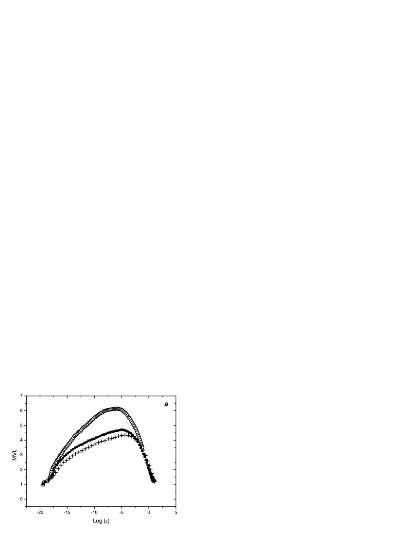
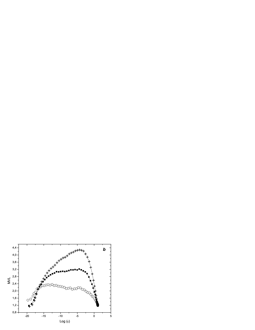
Figure 6: MVL graphics varying (a)$F_{Med}$ parameter, Open circle $F_{Med}=5$, Square $F_{Med}=6$ and Cross $F_{Med}=8$, for $N=128$ . (b)System Size. Open circle $N=32$, Square $N=64$ and Cross $N=128$. Common parameters, $\Delta$=0, $Amp=10^{-8}$.

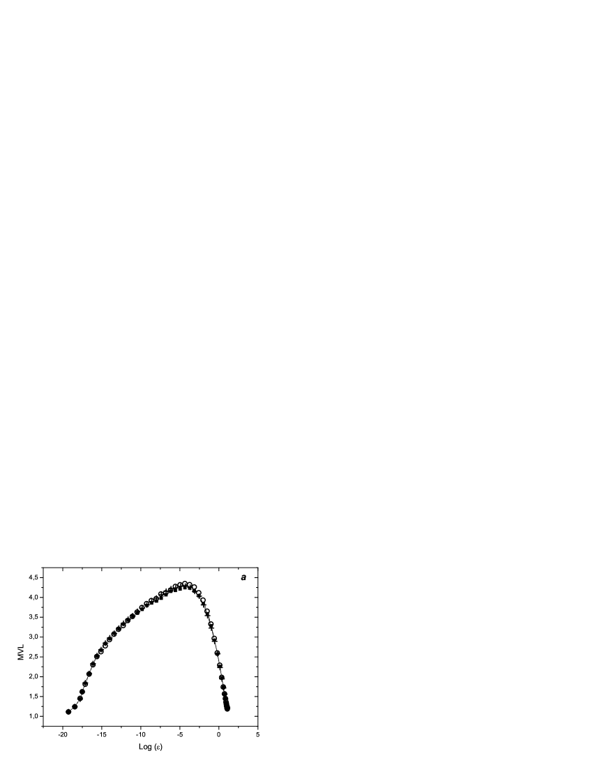
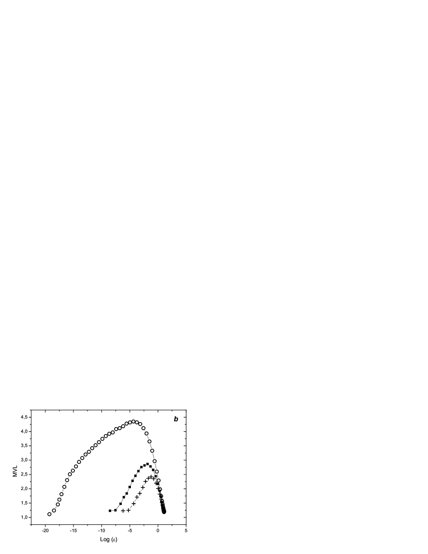
Figure 7: MVL graphics for (a) perturbations evolution. (b) errors evolution. Open circle corresponds to non-noise evolution $\Delta=0$, square to $\Delta=0.001$ and cross to $\Delta=0.01$. Common parameters, $N=128$, $F_{Med}=8.0$, $Amp=10^{-8}$.

V Conclusions

We have investigated the effect of a time-correlated noise on an extended chaotic system, analyzing the competence between the indicated deterministic or pseudo-noise and the real random process. For our study we have chosen the Lorenz’96 model Lor96-1 that, in spite of the fact that it is a kind of toy model, is of interest for the analysis of climate behavior Lor96-2 ; Lor96-3 . It is worth remarking that it accounts in a simple way for the spatial structure of geostrophic waves and the dynamics of tropical winds. The time series obtained at a generic site $x_{i}(t)$ mimics the passing of such waves, which is in fact a typical forecast event. We have assumed that the unique model parameter $F$ is time dependent and composed of two parts, a constant deterministic, and a stochastic contribution in both temporal and spatiotemporal forms.

We have done a thorough analysis of the system’s temporal evolution and its time correlations. The action of a stochastic noise on the Lorenz’96 system produces a dissipation on the time evolution. This dissipation essentially depends on the $F_{Med}$ parameter. Furthermore our results show numerical evidence for two SR-like behaviors. In one hand a “normal” SR phenomenon that occurs at frequencies that seems to correspond to a system’s quasi-periodic behavior. On the other hand, we have found a SSSR-like behavior, indicating that there is an optimal system size for the analysis of the spatial system’s response. As indicated before, the effect of noise is stronger when the chaos is underdeveloped.

We argue that these findings are of interest for an optimal climate prediction. It is clear that the inclusion of the effect of an external noise, that is a stochastic parametrization of unknown external influences, could strongly affect the deterministic system response, particularly through the possibility of an enhanced system’s response in the form of resonant-like behavior. It is worth here remarking the excellent agreement between the resonant frequencies and wave length found here, and the estimates of Lorenz Lor96-1p .

The effect of noise is weak respect to changes in the spatial structure, with the main frequencies remaining unaltered, but it is strong concerning the strength of the “self-generated” deterministic noise. We expect that in such a system and at the resonant frequencies, forecasting would be improved by the external noise due to the effect of suppression of the self-generated chaotic noise. Such an improvement will become apparent through the analysis of the localization phenomenon in the MVL diagrams. The detailed analysis of such an aspect will be the subject of a forthcoming study nos1 .

Acknowledgments: We acknowledge financial support from MEC, Spain, through Grant No. CGL2004-02652/CLI. JAR thanks the MEC, Spain, for the award of a Juan de la Cierva fellowship. HSW thanks to the European Commission for the award of a Marie Curie Chair during part of the development of this work.

References

- (1) L. Gammaitoni, P. Hänggi, P. Jung and F. Marchesoni, Rev. Mod. Phys. 70, 223 (1998).
- (2) J. F. Lindner, B. K. Meadows, W. L. Ditto, M. E. Inchiosa and A. Bulsara, Phys. Rev. E 53, 2081 (1996);
- (3) H. S. Wio, Phys. Rev. E 54, R3045 (1996); F. Castelpoggi and H. S. Wio, Europhys. Lett. 38, 91 (1997); F. Castelpoggi and H. S. Wio, Phys. Rev. E 57, 5112 (1998); S. Bouzat and H. S. Wio, Phys. Rev. E 59, 5142 (1999); H. S. Wio, S. Bouzat and B. von Haeften, in Proc. 21st IUPAP International Conference on Statistical Physics, STATPHYS21, A.Robledo and M. Barbosa, Eds., published in Physica A 306C 140-156 (2002).
- (4) W. Horsthemke and R. Lefever, Noise-Induced Transitions: Theory and Applications in Physics, Chemistry and Biology, (Springer, Berlin, 1984).
- (5) C. Van den Broeck, J. M. R. Parrondo and R. Toral, Phys. Rev. Lett. 73, 3395 (1994); C. Van den Broeck, J. M. R. Parrondo, R. Toral and R. Kawai, Phys. Rev. E 55, 4084 (1997).
-
(6)
S. Mangioni, R. Deza, H. S. Wio and R. Toral,
Phys. Rev. Lett. 79, 2389 (1997);
S. Mangioni, R. Deza, R. Toral and H. S. Wio, Phys. Rev. E 61, 223 (2000). - (7) P. Reimann, Phys. Rep. 361, 57 (2002); R. D. Astumian and P. Hänggi, Physics Today, 55 (11) 33 (2002).
- (8) P. Reimann, R. Kawai, C. Van den Broeck and P. Hänggi, Europhys. Lett. 45, 545 (1999); S. Mangioni, R. Deza and H.S. Wio, Phys. Rev. E 63, 041115 (2001).
- (9) J. García-Ojalvo, A. Hernández-Machado and J. M. Sancho, Phys. Rev. Lett. 71, 1542 (1993); J. García-Ojalvo and J. M. Sancho, Noise in Spatially Extended Systems (Springer-Verlag, New York, 1999).
- (10) B. von Haeften and G. Izús, Phys. Rev. E 67, 056207 (2003), G. Izús, P. Colet, M. San Miguel and M. Santagiustina, Phys. Rev. E 68, 036201 (2003).
- (11) S. Mangioni and H. S. Wio, Phys. Rev. E 67, 056616 (2003).
- (12) J. García-Ojalvo and J. M. Sancho, Noise in Spatially Extended Systems (Springer-Verlag, New York, 1999).
- (13) T. Bohr, M.H. Jensen, G. Paladin and A. Vulpiani, Dynamical Systems Approach to Turbulence, (Cambridge U.P., Cambridge, 1998).
- (14) J.M. Gutiérrez, A. Iglesias and M.A. Rodríguez, Phys. Rev. E 48, 2507 (1993); H. Wang and Q. Ouyang, Phys. Rev. E 65 046206 (2002); G. A. Gottwald and I. Melbourne, Physica D 212, 100 (2005); G. Ambika, K. Menon and K.P. Harikrishnan, Europhys. Lett. 73, 506 (2006).
- (15) V. S. Anishchenko, A. B. Neiman and M. A. Safanova, J. Stat. Phys. 70, 183 (1993); V. S. Anishchenko, M. A. Safanova and L. O. Chua, Int. J. Bifurcation and Chaos Appl. Sci. Eng. 4, 441 (1994).
- (16) D. Hennig, L. Schimansky-Geier and P. Hänggi, Europhys. Lett. 78, 20002 (2007).
- (17) D. S. Wilks, Quaterly J. of the Royal Meteor. Soc. B 131, 389 (2005)
- (18) E. N. Lorenz, The essence of chaos, (U.Washington Press, Washington, 1996).
- (19) E. N. Lorenz and K. A. Emanuel, J. Atmosph. Sci. 55, 399 (1998).
- (20) D. Orrell, J. Atmosph. Sci. 60, 2219 (2003)
- (21) N. van Kampen; Stochastic Processes in Physics and Chemistry, (North Holland, 1982)
- (22) C. W. Gardiner; Handbook of Stochastic Methods, 2nd Ed. (Springer-Verlag, Berlin, 1985).
- (23) B. von Haeften, G. G. Izús and H. S. Wio, Phys. Rev. E 72, 021101 (2005).
- (24) H. Gang, T. Ditzinger, C.Z. Ning and H. Haken, Phys. Rev. Lett. 71, 807 (1993); S. Zhong and H. Xin, J. Phys Chem. 104, 297 (2000); A. F. Rosenfeld, C. J. Tessone, E. Albano and H. S. Wio, Phys. Lett. 280, 45 (2001).
- (25) A. Pikovsky and A. Politi, Nonlinearity 11, 1049 (1998).
- (26) J. M. López, C. Primo, M. A. Rodriguez and I. Szendro, Phys. Rev. E 70, 056224 (2004).
- (27) C. Primo, I. Szendro, M. A. Rodriguez and J. M. Gutiérrez, Phys. Rev. Lett. 98, 108501 (2007).
- (28) C. Primo, M. A. Rodriguez, J. M. López and I. Szendro, Phys. Rev. E 72, 015201(R) (2005).
- (29) C. Primo, I. Szendro, M. A. Rodriguez and J. M. López, Europhys. Lett. 76, 767 (2006).
- (30) J. M. Gutiérrez, C. Primo, M. A. Rodriguez and J. Fernández, submitted to Geophys. Res. Lett.
- (31) J. A. Revelli, M. A. Rodriguez and H. S. Wio, to be submited to Europ. Phys. J. B.