Dynamical and energetic instabilities in multi-component Bose-Einstein condensates in optical lattices

Abstract

We study dynamical and energetic instabilities in the transport properties of Bloch waves for atomic multi-component Bose-Einstein condensates in optical lattices in the tight-binding limit. We obtain stability criteria analytically, as a function of superfluid velocities and interaction parameters, in several cases for two-component and spinor condensates. In the two-species case we find that the presence of the other condensate component can stabilize the superfluid flow of an otherwise unstable condensate and that the free space dynamical miscibility condition of the two species can be reversed by tuning the superfluid flow velocities. In spin-1 condensates, we find the steady-state Bloch wave solutions and characterize their stability criteria. We find generally more regions of dynamical instability arise for the polar than for the ferromagnetic solutions. In the presence of magnetic Zeeman shifts, we find a richer variety of condensate solutions and find that the linear Zeeman shift can stabilize the superfluid flow in several cases of interest.

I Introduction

There has been considerable recent interest in the dynamical properties of atomic Bose-Einstein condensates (BECs) in optical lattice potentials AND98 ; BUR01 ; MOR01 ; josephson ; CAT03 ; CRI04 ; FAL04 ; FER05 ; SAR05 ; TUC06 ; FER07 ; WU01 ; SME02 ; WU03 ; ZHE04 ; MON04 . In optical lattices the nonlinear mean-field interaction of the BEC may give rise to dynamical and energetic instabilities in the transport properties of the atoms. For a single-component condensate, when the center-of-mass (CM) velocity reaches a critical value, the BEC dynamics become unstable resulting in an abrupt stop of the transport of the atom cloud in the lattice. Such a superfluid to insulator transition has a classical nature and it can be described using the Gross-Pitaevskii (GP) mean-field models WU01 ; SME02 ; WU03 ; MON04 . In the dynamically unstable regime small initial perturbations around a moving solution grow exponentially in time, resulting in the randomization of the relative phases between atoms in adjacent lattice sites. The dynamical transition to inhibited atom transport was experimentally observed in the classical regime BUR01 ; CAT03 ; CRI04 ; FAL04 ; SAR05 and experimental methods to characterize both the dynamical and energetic instabilities of moving condensates have been developed SAR05 . Inhibition of transport was also observed in the presence of large quantum fluctuations using strongly confined narrow atom tubes FER05 . In a confined system with enhanced quantum fluctuations the sharp classical transition is smeared out POL04 ; RUO05 ; BAN06 , resulting in a gradually increasing friction in the atom transport. Due to the broadening of the velocity distribution of the atoms, even at low velocities a non-negligible atom population occupies the dynamically unstable high velocity region of the corresponding classical system, generating in the shallow lattice limit the friction RUO05 ; POL05 .

Despite this work on single-component condensates, there have been relatively few studies of dynamics of multi-component BECs in optical lattices. Due to nearly equal trapping potentials of different Zeeman sub-levels (for example $F=1,m_{F}=-1$ and $F=2,m_{F}=1$ in ²³Na and ⁸⁷Rb), it is possible to create long-lived two component BECs, forming an effective spin-1/2 system. These have especially long lifetimes in ⁸⁷Rb due to a fortuitous cancelation of scattering lengths VOG02 . This additional degree of freedom has been utilized to study an interesting array of effects in both Bose-condensed and non-condensed cold Bose systems, including phase separation HALL98 , optically-induced shock waves DUT01 , spin waves LEW02 ; NIK03 , overlapping ⁴¹K–⁸⁷Rb BEC mixtures MOD02 , spin squeezing SOR01 , and vector soliton structures RUO01 ; BUS01 ; SAV03 . Experimental work on two-component BECs in optical lattices, from the viewpoint of quantum logic gates, was reported in MAN03 . There has also been a recent experimental realization a two-species ⁴¹K–⁸⁷Rb Bose mixture in an optical lattice CAT07 .

Alternatively, in dipole traps STE98 the spin of the atom is no longer constrained by the magnetic field and, due to the additional atomic spin degrees of freedom, the BEC exhibits a richer spinor order parameter structure. The spin of the optically trapped BECs can generally have significant effects on the dynamical properties of the BECs STE98 ; MIE99 , give rise to spin textures LEA03 , and support of highly nontrivial defect structures ZHO03 ; RUO03 ; MUE04 ; REI04 . Experiments have also explored dynamics in spinor condensates in harmonic traps SCH04 ; CHA04 ; KRO05 ; BLA07 and optical lattices WID05 , and the application of spinor gases to spatially resolved magnetometry VEN07 .

In this paper we investigate both dynamical and energetic instabilities in the transport of multi-component BECs in optical lattices. We first consider magnetically trapped two-component BECs where the two condensates occupy different hyperfine states of the same atom or are formed by mixtures of two different atoms. Transport properties of two-component BECs in an optical lattice were studied in Ref. HOO06 , and numerical results for dynamical instabilities were presented for a special case. In particular, dynamical instabilities were shown to arise from the critical velocity as well as from the phase separation of the two species. In contrast to that work, we obtain analytic results for the condensate dynamical instability points and analyze in detail the complete phase space of stability criteria for both dynamical and energetic instabilities across a broad range of parameters. We vary the intra- and inter-species interaction strengths, the site hopping term for each spin component independently, as well as the velocities of the two BECs, allowing application of our results to a large variety of experimental systems. Among the novel results presented here are the possibility of a second BEC component stabilizing the superfluid flow of an otherwise unstable first BEC component (that exceeds the critical velocity of a single-component BEC). In addition, we find the free space phase separation criteria, that the square of the inter-species interaction coefficient exceeds the product of the intra-species interaction coefficients ($U_{12}^{2}>U_{11}U_{22}$), can be reversed in an optical lattice. This can happen if one of the BECs has a velocity larger and the other one smaller than the single-species critical velocity (the effective masses of the two components exhibit different signs).

We also analyze transport properties of optically trapped spin-1 BECs in optical lattices, which have not been experimentally investigated to date. Here we obtain analytic expressions for both the dynamical and energetic instability regions of the Bloch wave solutions. In contrast to the two-component case, spin changing collisions allow the atom population of different spin components to adjust to lower the energy of the system, according to whether the scattering lengths correspond to polar or ferromagnetic values. Our results illuminate the different stability properties of the polar versus ferromagnetic solutions, which, in the absence of the Zeeman shifts, are most apparent for large spin-dependent scattering lengths or when the spin-dependent and spin-independent scattering lengths exhibit different signs. The presence of the Zeeman level shifts provides a richer variety of steady-state Bloch wave solutions, including novel solutions that do not exist for the case of small level shifts. We find that the quadratic Zeeman shift, due to its role in the energy conservation of spin changing collisions, plays an important role in the stability of various condensate solutions. However, we also see that linear Zeeman shifts play an important role in stabilizing many of the solutions. The dynamical instabilities of the spinor BECs can be important, e.g., also in the formation of solitons that have been studied in the homogeneous case in Ref. DAB07 .

In Sec. II we introduce the discrete nonlinear Schrodinger equation and the Bogoliubov-de Gennes approach to study the stability properties of condensate solutions. This is done in the context of the two-component case but the same method is used later for the spinor case. We then derive expressions for the normal mode energies and discuss the dynamical and energetic stability of the two-component case. In Sec. III we apply this method to the spinor case. We first discuss the polar case, then the ferromagnetic case, then finally the effect of the Zeeman shifts. Some experimental considerations for observation of the effects studied are discussed in Sec. IV. We summarize our results in Sec. V. The Bogoliubov-de Gennes matrices are presented explicitly in Appendix A and the detailed analysis of the stability of the two-component case when the phase separation condition is reversed is given in Appendix B.

II A two-component condensate in an optical lattice

II.1 Two species system description

Two-component BECs can be prepared in magnetic traps by simultaneously confining different atomic species in the same trap. The atoms may occupy two different hyperfine states of the same atomic species or form a mixture of two condensates of two different atomic species. For instance, two BEC components in perfectly overlapping isotropic magnetic trapping potentials were experimentally realized in hyperfine spin states of ⁸⁷Rb, $|\uparrow\rangle\equiv|F=2,m_{f}=1\rangle$ and $|\downarrow\rangle\equiv|F=1,m_{f}=-1\rangle$. In this system the inter- ($a_{\uparrow\downarrow}$) and intraspecies ($a_{\uparrow\uparrow}$ and $a_{\downarrow\downarrow}$) interaction strengths are nearly equal, with $a_{\downarrow\downarrow}:a_{\uparrow\downarrow}:a_{\uparrow\uparrow}::1.024:1:0.973$ HAR02 . Since the scattering lengths satisfy $a_{\uparrow\downarrow}^{2}\gtrsim a_{\uparrow\uparrow}a_{\downarrow\downarrow}$, the two species experience dynamical phase separation and can strongly repel each other HALL98 . A more strongly repelling two-component system of different species was created using a ⁴¹K–⁸⁷Rb mixture MOD02 . The interatomic interactions of two magnetically trapped BEC components do not mix the atom population and the atom numbers of both species are separately conserved.

The dynamics of the BECs follow from the coupled Gross-Pitaevskii equation (GPE)

$$i\hbar{\partial\psi_{j}\over\partial t}=(-{\frac{\hbar^{2}}{2m_{j}}}{\bf\nabla}^{2}+V_{j}({\bf r})+\sum_{k}\kappa_{jk}|\psi_{k}|^{2})\psi_{j}\,.$$ (1)

Here we have defined the interaction coefficients $\kappa_{ii}\equiv 4\pi\hbar^{2}a_{ii}/m_{i}$ and $\kappa_{ij}\equiv 2\pi\hbar^{2}a_{ij}/\mu$ ($i\neq j$), where the wavefunctions are normalized to $N_{j}$, $N=N_{1}+N_{2}$ is the total atom number, $m_{j}$ is the atomic mass of BEC component $|j\rangle$, and $\mu=m_{1}m_{2}/(m_{1}+m_{2})$ is the reduced mass. The intraspecies and the inter species scattering lengths are denoted by $a_{ii}$ and $a_{ij}$ ($i\neq j$), respectively. The external potential is generally a superposition of a harmonic trapping potential $V_{H}^{(j)}({\bf r})=m(\omega_{jx}^{2}x^{2}+\omega_{jy}^{2}y^{2}+\omega_{jz}^{2}z^{2})/2$ and the periodic optical lattice potential $V_{L}^{(j)}({\bf r})=V_{0}^{(j)}\sin^{2}(\pi x/a+\varphi_{j})$, $V_{j}({\bf r})=V_{H}^{(j)}({\bf r})+V_{L}^{(j)}({\bf r})$, where $a$ denotes the lattice spacing. In the following we ignore the effect of the harmonic trapping potential along the lattice and consider the system as translationally invariant. We also neglect density fluctuations orthogonal to the optical lattice and consider the dynamics as effectively 1D.

We write the GPE in the tight-binding approximation by expanding the BEC wavefunctions on the basis of the Wannier functions and only keep the lowest vibrational states in each lattice site $\eta$, so that $\psi_{j}({\bf r})=\sum_{\eta}c^{(j)}_{\eta}\phi_{j\eta}({\bf r})$ JAK98 . We obtain discrete nonlinear Schrödinger equations (DNLSEs):

$$i\hbar{dc^{(j)}_{\eta}\over dt}=-J_{j}(c^{(j)}_{\eta+1}+c^{(j)}_{\eta-1})+\sum_{k}U_{jk}|c^{(k)}_{\eta}|^{2}c^{(j)}_{\eta}\,.$$ (2)

With similar assumptions, we have the hopping amplitude, $J_{j}>0$, for the atoms between adjacent lattice sites:

$$J_{j}\simeq-\int d^{3}r\,({\hbar^{2}\over 2m_{j}}\nabla\phi_{j\eta}^{*}\cdot\nabla\phi_{j,\eta+1}+\phi_{j\eta}^{*}V_{L}^{(j)}\phi_{j,\eta+1})\,.$$ (3)

The nonlinearities are given by $U_{jk}\simeq\kappa_{jk}\int d^{3}r\,|\phi_{j\eta}|^{2}|\phi_{k\eta}|^{2}$. The two BEC species may generally experience different lattice potentials MAN03 and so the interspecies coupling coefficient $U_{12}$ may be varied by displacing the two lattice potentials with respect to each other (to modify the overlap integral between the wavefunctions), even when the values of the scattering lengths remain constant; Fig. 1.

Figure 1: The two BECs may experience different optical lattice potentials that can be shifted with respect to each other. The interspecies interaction strength $U_{12}$ is proportional to the overlap integral of the two lattice site mode functions and it can be adjusted by shifting the lattices. Moreover, the kinetic energy hopping amplitude of the two species $J_{1},J_{2}$ may be independently modified by changing the barrier height between the neighboring sites.

II.2 Dynamical stability of two species

II.2.1 Collective two-component excitations

We study the stability of plane wave solutions to Eq. (2) by investigating the effect of small perturbations around the carrier wave. Our treatment is analogous to the approach in Ref. SME02 to analyze single-component BECs. For the constant atom density along the lattice, the Bloch waves $c^{(j)}_{\eta}=\sqrt{n_{j}}\exp{[i(k_{j}a\eta-\nu_{j}t)]}$ that satisfy Eq. (2) exhibit the frequency $\nu_{j}=\sum_{i}n_{i}U_{ji}-2J_{j}\cos(k_{j}a)$, where $n_{j}=|c^{(j)}_{\eta}|^{2}$ denotes the constant atom population in spin state $j$ at each site. The perturbed carrier wave can be written as a Bogoliubov expansion:

$$c^{(j)}_{\eta}=(\sqrt{n_{j}}+u_{j}e^{iqa\eta}-v_{j}^{*}e^{-iqa\eta})e^{i(k_{j}a\eta-\nu_{j}t)}\,.$$ (4)

Here the $k_{j}$ represent the potentially non-zero velocities of the condensate in each component $j$. The stability of such states in a single component BEC has been studied experimentally in Refs. FAL04 ; SAR05 by dynamically moving the lattice potential. Substituting this expansion into Eq. (2) and linearizing the equations in $u_{1}$, $v_{1}$, $u_{2}$, and $v_{2}$ yields a system of four equations

$$i{d\over dt}{\bf x}=\sigma{\cal M}(q){\bf x},\quad{\bf x}=\begin{pmatrix}u_{1}\\ v_{1}\\ u_{2}\\ v_{2}\end{pmatrix},\quad\sigma=\left(\begin{array}[]{cc}\sigma_{z}&0\\ 0&\sigma_{z}\end{array}\right)\,,$$ (5)

where $\sigma_{z}$ denotes the $2\times 2$ Pauli spin matrix. The elements of the $4\times 4$ matrix ${\cal M}(q)$ follow from the linearization procedure as in the single-component BEC case. We write out this matrix explicitly in Appendix A. The eigenvalue problem for the matrix $\sigma{\cal M}(q)$ can be solved analytically. In order to preserve the symmetry properties the Bogoliubov equations and to obtain simple analytic expressions for the normal mode energies we require that the atom currents of the two BECs are equal, i.e., $J_{1}\sin(k_{1}a)=J_{2}\sin(k_{2}a)$.

The eigenvalues represent the normal mode energies and read

$$\omega_{q}=2J_{1}\sin(k_{1}a)\sin(qa)\pm\sqrt{\hbox{$1\over 2$}(\omega_{1,q}^{2}+\omega_{2,q}^{2})\pm\hbox{$1\over 2$}\sqrt{(\omega_{1,q}^{2}-\omega_{2,q}^{2})^{2}+16\epsilon_{1,q}\cos(k_{1}a)\epsilon_{2,q}\cos(k_{2}a)n_{1}n_{2}U_{12}^{2}}}\,.$$ (6)

The four eigenvalues correspond to all permutations of the $\pm$ signs. Only two of the eigenvalues are independent. The first term in Eq. (6) represents the Doppler shift of the excitation energies due to the superfluid current. Here $\omega_{j,q}$ denotes the single-condensate normal mode energies (without the Doppler shift term)

$$\omega_{j,q}^{2}=\epsilon_{j,q}\cos(k_{j}a)[\epsilon_{j,q}\cos(k_{j}a)+2n_{j}U_{jj}]\,,$$ (7)

and

$$\epsilon_{j,q}=4J_{j}\sin^{2}\left({qa\over 2}\right)\,,$$ (8)

is the spectrum of an ideal, non-moving BEC.

For the case of positive definite ${\cal M}(q)$ all the eigenvalues $\omega_{q}$ of $\sigma{\cal M}(q)$ are real. In that case the physical solutions of the corresponding eigenvectors ${\bf y}$ exhibit positive normalization ${\bf y}^{\dagger}\sigma{\bf y}=1$ (the ‘$+$’ sign in the front of the first square root) and unphysical eigenvectors negative normalization ${\bf y}^{\dagger}\sigma{\bf y}=-1$ (the ‘$-$’ sign in the front of the first square root). The eigenvalues $\omega_{q}$ with a nonvanishing imaginary part are associated with eigenvectors satisfying ${\bf y}^{\dagger}\sigma{\bf y}=0$. The BEC system becomes dynamically unstable when the normal mode frequencies in Eq. (6) exhibit nonvanishing imaginary parts, indicating perturbations that grow exponentially in time. Such modulational instabilities occur in a closed system due to the nonlinear dynamics and do not require energy dissipation. The rate at which the instability sets in depends on the magnitude of the imaginary part of the eigenfrequency.

For small momenta, $qa\ll 1$, $\epsilon_{j,q}\simeq J_{j}q^{2}a^{2}=\hbar^{2}q^{2}/2m_{j}^{*}$, where we introduced the effective mass of a noninteracting BEC as $m_{j}^{*}=\hbar^{2}/(2J_{j}a^{2})$. Similarly, we obtain $2J_{1}\sin(k_{1}a)\sin(qa)\simeq 2J_{1}k_{1}qa^{2}=\hbar^{2}k_{1}q/m_{1}^{*}$ reinforcing the interpretation of the first term in Eq. (6) as the Doppler shift contribution.

If we set $U_{12}=0$ in Eq. (6), we obtain independently the decoupled normal mode energies of the two BECs $\omega_{q}=2J_{1}\sin(k_{1}a)\sin(qa)+|\omega_{1,q}|$ and $\omega_{q}=2J_{1}\sin(k_{1}a)\sin(qa)+|\omega_{2,q}|$, analogously to the single-condensate normal modes obtained in Ref. SME02 .

The intraspecies interaction $U_{12}$ mixes the normal modes of the two BECs. In the experimentally interesting regime $n_{j}U_{jj}\gg J_{j}$, if $U_{12}^{2}\simeq U_{11}U_{22}$, one of the frequencies approaches zero indicating an instability similar to the uniform two-component BEC system. Specifically, for $k_{1}=k_{2}=0$, we obtain in that case $\omega_{q,+}^{2}\simeq\omega_{1,q}^{2}+\omega_{2,q}^{2}$ and $\omega_{q,-}^{2}\ll\omega_{1,q}^{2},\omega_{2,q}^{2}$.

By expanding $\omega_{q}$ for small $q$ in Eq. (6) with $k_{1}=k_{2}=0$, we obtain $\omega_{q}\simeq\hbar sq$ where $s$ is the speed of sound

$$s_{\pm}={a\over\hbar}\sqrt{J_{1}n_{1}U_{11}+J_{2}n_{2}U_{22}\pm\sqrt{(J_{1}n_{1}U_{11}-J_{2}n_{2}U_{22})^{2}+4J_{1}J_{2}n_{1}n_{2}U_{12}^{2}}}\,.$$ (9)

The long wavelength excitations are unstable when one of the solutions for the speed of sound has an imaginary part.

If we do not assume that the two BEC currents are equal $J_{1}\sin(k_{1}a)\neq J_{2}\sin(k_{2}a)$, the Doppler shifts for the two BECs are different and the usual symmetry properties between the positive and the negative energy Bogoliubov eigenfunctions are lost. We still find analytic solutions for the eigenenergies $\omega_{q}$, but these no longer have simple compact expressions as in Eq. (6). The basic formalism may be used to generate stability diagrams in these cases numerically, for instance, even if the two BECs have the velocities in the opposite directions. In the following we concentrate on analyzing the general features of the two-component system that may already be obtained from Eq. (6).

II.2.2 Stability with equal signs for $\cos(k_{1}a)$ and $\cos(k_{2}a)$

We first analyze the dynamical stability of the two-component system, given in Eq. (6) for $J_{1}\sin(k_{1}a)=J_{2}\sin(k_{2}a)$, for the case that $\cos(k_{1}a)$ and $\cos(k_{2}a)$ exhibit equal sign. For that case, the expression inside the square root in Eq. (6) is always negative (for any values of $U_{12}$), and the dynamics unstable, if $\omega_{1,q}^{2}+\omega_{2,q}^{2}<0$. Physically, this corresponds to the situation where the two-component dynamical instability is driven by the instabilities of the individual single-component BEC excitations (7). We have $\omega_{1,q}^{2}+\omega_{2,q}^{2}<0$, for some values of $q$, if

$$\sin^{2}{\left({qa\over 2}\right)}<-{D_{11}+D_{22}\over 2[J_{1}^{2}\cos^{2}{(k_{1}a)}+J_{2}^{2}\cos^{2}{(k_{2}a)}]}\,,$$ (10)

where

$$D_{ij}=J_{i}\cos(k_{i}a)n_{j}U_{jj}\,.$$ (11)

The inequality is most easily satisfied for excitations in the long-wavelength limit $q\rightarrow 0$, and is satisfied when the right hand side is positive, i.e., for

$$D_{11}+D_{22}<0\,.$$ (12)

According to Eq. (12), the modes can become unstable if $k_{1}a,k_{2}a>\pi/2$ even when $U_{11},U_{22}>0$, which is the usual high velocity instability seen in the single component case WU01 . The dynamics can also be unstable when $k_{1}a,k_{2}a<\pi/2$, for negative values of $U_{11}$ and $U_{22}$.

In addition to the instability occurring for $\omega_{1,q}^{2}+\omega_{2,q}^{2}<0$, the two-component system in Eq. (6) is always dynamically unstable (for the case that $\cos(k_{1}a)$ and $\cos(k_{2}a)$ exhibit equal sign) if

$$U_{12}^{2}>U_{11}U_{22}\,,$$ (13)

as the expression in the outer square root in Eq. (6) becomes negative. In particular, the unstable $q$ modes are those that satisfy (when $\omega_{1,q}^{2}+\omega_{2,q}^{2}\geq 0$):

$$\sin^{2}{\left({qa\over 2}\right)}<{-(D_{12}+D_{21})+\sqrt{(D_{12}-D_{21})^{2}+4J_{1}\cos(k_{1}a)J_{2}\cos(k_{2}a)n_{1}n_{2}U_{12}^{2}}\over 4J_{1}\cos(k_{1}a)J_{2}\cos(k_{2}a)}\,.$$ (14)

The two-component system, consequently, is in this case dynamically stable if $D_{11}+D_{22}>0$ and $U_{12}^{2}\leq U_{11}U_{22}$.

The unstable dynamics for $U_{12}^{2}>U_{11}U_{22}$ correspond to the analogous instability which occurs in the free space case due to phase separation. One should emphasize, however, that the value of $U_{12}$ is not only determined by the inter-species scattering length, but also by the spatial overlap integral of the lattice site wavefunctions for the two species; see the definition of $U_{ij}$ below Eq. (3). By means of shifting the relative position of the two BEC lattice potentials, one may easily reduce the value of $U_{12}$.

Phase space diagrams of the dynamical instability strengths as a function of the excitation wavelength $q$ and condensate wave number $k$ are shown in Fig. 2. In Fig. 2(a) we see the system is stable for the case $n_{c}U_{12}=8J_{1}$, $n_{1}U_{11}=n_{2}U_{22}=10J_{1}$ (defining $n_{c}=\sqrt{n_{1}n_{2}}$) when $ka<0.5\pi$, then becomes unstable for $ka>0.5\pi$, in accordance with Eq. (12). The strength of the instabilities (the largest imaginary part of the eigenvalues) are linear in $q$ [for the slope, see Eq. (9)] until they saturate approximately at a value ${\rm Im}(\omega_{q})\simeq\sqrt{-16n_{c}U_{12}J_{1}\cos{(k_{1}a)}}$, which is $\approx 11J_{1}$ at $ka=\pi$ in Fig 2(a). The strongest instability at $ka=\pi$ represents period doubling that drives the system away from the Bloch state. The behavior is qualitatively similar for all $n_{c}U_{12}\leq n_{1}U_{11}=n_{2}U_{22}$ and also for smaller values of $J_{1}$ and $J_{2}$. However, for $n_{c}U_{12}>n_{1}U_{11}$ [Fig. 2(b)], we see the predicted phase separation instability arises in the $ka<0.5\pi$ region. It is interesting to note this instability is markedly weaker than the high velocity instability ($ka>0.5\pi$), as its maximum value (occurring for $k=0$, $qa=\pi$) scales as ${\rm Im}(\omega_{q})\simeq\sqrt{8(n_{c}U_{12}-n_{1}U_{11})J_{1}}$ (in the limit that $n_{c}U_{12}-n_{1}U_{11}\gg J_{1}$). In the case plotted in Fig. 2(b), the value saturates at $\approx 3J_{1}$, whereas the instability strength in the $ka>0.5\pi$ region reaches $\approx 13J_{1}$.

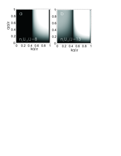
Figure 2: (a) Largest imaginary part of the eigenvalues Eq. (6) as function of $k\equiv k_{1}=k_{2}$ and $q$ for the case $n_{1}U_{11}=n_{2}U_{22}$, $n_{c}U_{12}=8J_{1}$ and $J_{2}=J_{1}$. We define $n_{c}\equiv\sqrt{n_{1}n_{2}}$. Gray scale goes from $0$ (black) to $5J_{1}$ (white). (b) Same plot with $n_{c}U_{12}=13J_{1}$ (phase separation regime).

Figures 3(a,b) compare the phase separation instability versus $n_{c}U_{12}$ for $k_{1}a=k_{2}a=0$ and $k_{1}a=k_{2}a=0.4\pi$. Generally speaking, the largest imaginary value reaches a maximum value ${\rm Im}(\omega_{q})\simeq\sqrt{8(n_{c}U_{12}-n_{1}U_{11})J_{1}}$. The dependence on the sign of $U_{11},U_{22}$ is shown in Fig. 4. We see in Fig. 4(a) that, for $n_{c}U_{12}<n_{1}U_{11}=n_{2}U_{22}$ and $\cos(k_{1}a)>0$, the instability is restricted to the attractive cases $U_{11}<0$. Fig. 4(b) demonstrates this instability switches to the repulsive case for $\cos(k_{1}a)<0$. Again these instabilities reach strengths ${\rm Im}(\omega_{q})\simeq\sqrt{16n_{1}U_{11}J_{1}}$. However, for the $\cos(k_{1}a)<0$ case there occurs also a much weaker instability for attractive interactions with strength ${\rm Im}(\omega_{q})\simeq\sqrt{8(n_{c}U_{12}-n_{1}U_{11})J_{1}}$.

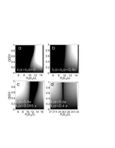
Figure 3: (a)-(b) Imaginary part of the eigenvalues versus $n_{c}U_{12}$ (again $n_{c}=\sqrt{n_{1}n_{2}}$), holding $n_{1}U_{11}=n_{2}U_{22}=10J_{1}$ for the indicated condensate velocities $k$. Here $J_{2}=J_{1}$ (c) A case with opposite signs of $\cos(k_{1}a)$ and $\cos(k_{2}a)$, showing a region of dynamical stability for all $q$. Here $n_{1}U_{11}=10J_{1}$, $n_{2}U_{22}=12J_{1}$ and $J_{2}=2J_{1}$. A similar narrow stable region exists around $n_{c}U_{12}\simeq-12J_{1}$. (d) Another case with opposite signs of $\cos(k_{1}a)$ and $\cos(k_{2}a)$. Here $n_{1}U_{11}=27J_{1}$, $n_{2}U_{22}=30J_{1}$ and $J_{2}=J_{1}$. Again another stable region in this case is located close to $n_{c}U_{12}\simeq-28.5J_{1}$. In these plots the gray scale goes from 0 to $5J_{1}$.

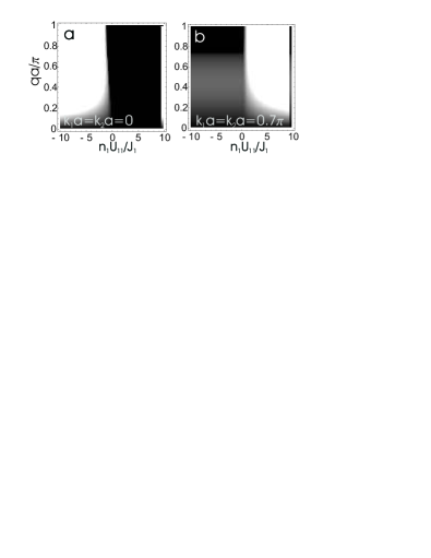
Figure 4: Imaginary part of the eigenvalues versus $q$ and varying $n_{1}U_{11}=n_{2}U_{22}$, keeping $n_{c}U_{12}=n_{1}U_{11}-J_{1}$ and with $J_{2}=J_{1}$. In this figure, the gray scale runs from 0 to $2.5J_{1}$.

II.2.3 Stability with different signs for $\cos(k_{1}a)$ and $\cos(k_{2}a)$

The case that $\cos{k_{1}a}$ and $\cos{k_{2}a}$ have different signs represents a configuration where the velocities of the two BECs are located on the opposite sides of the deflection point in the ideal, single-particle BEC excitation spectrum (8) (the effective masses of the two components exhibit different signs) and is presented in detail in Appendix B. In that situation, we also always find a dynamical instability when $\omega_{1,q}^{2}+\omega_{2,q}^{2}<0$, resulting in the relation similar to Eq. (12). In this case, however, the high velocity instability condition is highly nontrivial, depending on the values of the hopping amplitudes, the interaction strengths, atom numbers, and the velocities: One of the BECs that reaches the single-component critical velocity $k_{1}a>\pi/2$ may, or may not, destabilize the two-component BEC system, depending on the parameter values. Moreover, for $\omega_{1,q}^{2}+\omega_{2,q}^{2}\geq 0$, the dynamical stability condition due to the phase separation of the non-moving system, $U_{12}^{2}<U_{11}U_{22}$, is reversed, so that the entire dynamically stable region occurs, when $U_{12}^{2}>U_{11}U_{22}$. In particular, we find in that case the system to be dynamically stable if $U_{12}$ satisfies, depending on the value of $U_{11}$, either $U_{11}U_{22}<U_{12}^{2}<\xi_{1}$ or $U_{11}U_{22}<\xi_{2}<U_{12}^{2}<\xi_{1}$, where $\xi_{1}$ and $\xi_{2}$ are defined in Eqs. (50) and (55). Interestingly, this also represents a situation where the other condensate component can stabilize the superfluid flow of an otherwise unstable condensate (exceeding the single-component critical velocity). Moreover, the two-component system may be dynamically stable even for $U_{11}<0$ and $U_{22}>0$, since in that case $U_{11}U_{22}<U_{12}^{2}$.

Figures 3(c-d) show cases with $\cos(k_{1}a)$ and $\cos(k_{2}a)$ of different sign [but satisfying the condition $J_{1}\sin(k_{1}a)=J_{2}\sin(k_{2}a)$]. For the parameters of Fig. 3(c) there is a range of $n_{c}U_{12}$ for which the system is dynamically stable. In this case $n_{1}U_{11}$ satisfies Eq. (53) and the dynamically stable region, according to Eq. (54), is $\xi_{2}<U_{12}^{2}<\xi_{1}$. The relevant quantities are $n_{c}\sqrt{\zeta_{2}}=11.5J_{1}$ and $n_{c}\sqrt{\zeta_{1}}=12.5J_{1}$ for this example. Note that the dynamical instabilities tend to be much weaker on the large $U_{12}$ side of this stability range. In Fig. 3(c) we have different hopping amplitudes $J_{1}\not=J_{2}$. Fig. 3(d) shows a case with a smaller range of stable $n_{c}U_{12}$ but with $J_{1}=J_{2}$. In this case $n_{1}U_{11}$ satisfies Eq. (51) and the dynamically stable region, according to Eq. (52), is for $U_{11}U_{22}<U_{12}^{2}<\xi_{1}$. Here $n_{c}\sqrt{U_{11}U_{22}}=28.46J_{1}$ and $n_{c}\sqrt{\zeta_{1}}=28.50J_{1}$.

II.3 Energetic stability

The energetic stability of the superfluid flow of the homogeneous two-component mixture depends on the properties of the energy functional. The second-order variations of the energy for small perturbations in the carrier wave are determined by the matrix ${\cal M}(q)$ and the system is energetically stable if ${\cal M}(q)$ is positive definite. If any of the eigenvalues of ${\cal M}(q)$ are negative, the system may relax to a state with lower energy by means of dissipative coupling to the environment. The rate at which such relaxation happens depends on the strength of the coupling, e.g., on the number of thermal atoms interacting with the condensate.

The eigenvalues of ${\cal M}(q)$ can also be evaluated analytically but the full solutions are rather lengthy. In Fig. 5 we show the energetically unstable regions of the two-component dynamics. Note that positive definite ${\cal M}(q)$ implies real eigenvalues $\omega_{q}$ of $\sigma{\cal M}(q)$ in Eq. (6), so the dynamically unstable region always forms a subset of the energetically unstable region. Figures 5(a-b) show cases with $n_{c}U_{12}<n_{1}U_{11}$ and $n_{c}U_{12}>n_{1}U_{11}$, respectively. In the latter case there are regions of instability for some $q$ at all condensate wavenumbers $k$. In the former case, there are is a band of $k$ with all $q$ modes energetically stable, with a width proportional to $\sqrt{2J_{1}(n_{1}U_{11}-n_{c}U_{12})}$, which determines the speed of sound for the spin wave; see Eq. (9) with $n_{1}U_{11}=n_{2}U_{22}$, $J_{1}=J_{2}$. This is analogous to the single-component case WU01 where there is a band of energetically stable $k$ with a width proportional to the speed of sound $\propto\sqrt{2J_{1}n_{1}U_{11}}$. In Figs. 5(c),(d) we show the dependence on $U_{12}$. It is seen that at $k=0$ instability only occurs for $U_{12}>U_{11}$ while for finite $k$ the condition for stability becomes more stringent. For $ka>0.5\pi$ the entire region is unstable. We also calculated that the specific parameter regimes corresponding to dynamical stability with two different condensate wavenumbers $k_{1},k_{2}$ (Figs. 3(c,d)) are energetically unstable at all $q$.

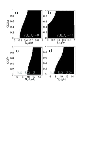
Figure 5: (a)-(b) Regions of energetic stability (white) and instability (black) versus $k_{1}$ and $q$ for the cases indicated. We choose $n_{1}U_{11}=n_{2}U_{22}=10J_{1}$, $J_{2}=J_{1}$ and $k_{2}=k_{1}$. (c)-(d) Energetic stability regions versus $n_{c}U_{12}$ for a stationary and moving condensate case.

III A spin-1 condensate in an optical lattice

III.1 Spinor Gross-Pitaevskii equations

We now consider a BEC of spin-1 atoms. In the absence of a magnetic trapping potential, the macroscopic BEC wave function is determined by a spinor wave function $\Psi$ with three complex components Pethick . The Hamiltonian density of the classical GP mean-field theory for this system reads:

$${\cal H}= \frac{\hbar^{2}}{2m}|\nabla\Psi|^{2}+V\rho+{c_{0}\over 2}\rho^{2}+{c_{2}\rho^{2}\over 2}|\langle{\bf F}\rangle|^{2}$$

$$+g_{1}\langle{\bf B}\cdot{\bf F}\rangle\rho+g_{2}\langle({\bf B}\cdot{\bf F})^{2}\rangle\rho\,,$$ (15)

In Eq. (III.1), ${\bf F}$ is the vector formed by the three components of the $3\times 3$ Pauli spin-1 matrices Pethick , $\langle{\bf F}\rangle=\Psi^{\dagger}\cdot{\bf F}\cdot\Psi/\rho$ denotes the average spin, and $\rho({\bf r})=|\Psi({\bf r})|^{2}$ the total atom density. The weak external magnetic field is denoted by ${\bf B}$ and is assumed to point along the $z$ axis. The magnetic field produces the linear and quadratic Zeeman level shifts whose effect is described by the last two terms in Eq. (III.1). As in the two-component case, the external potential $V$ is the sum of the harmonic part $V_{H}$ (in this case due to the optical dipole trap) and the optical lattice potential $V_{L}$: $V({\bf r})=V_{H}({\bf r})+V_{L}({\bf r})$. In the following we ignore the harmonic potential and, for simplicity, assume that the lattice potential is the same for all the spinor components. Thus the Wannier basis functions $\phi_{\eta}$ of our discrete basis no longer depend on the internal state $j$. Here $c_{0}$ and $c_{2}$ are the spin-independent and spin-dependent two-body interaction coefficients. In terms of the s-wave scattering lengths $a_{0}$ and $a_{2}$, for the channels with total angular momentum zero and two, they are: $c_{0}\equiv 4\pi\hbar^{2}(2a_{2}+a_{0})/3m$, and $c_{2}\equiv 4\pi\hbar^{2}(a_{2}-a_{0})/3m$. For ²³Na, $(a_{2}-a_{0})/3\simeq 2a_{B}$ and $(2a_{2}+a_{0})/3\simeq 50a_{B}$, where $a_{B}=0.0529$ nm is the Bohr radius Pethick , indicating $c_{2}/c_{0}\simeq 0.04$. In contrast to the two-component case, in which the atom number in the two-components do not mix, in the spinor case a homogenous condensate wavefunction can adjust itself by varying the relative atom populations. From Eq. (III.1) in the absence of the external magnetic field we immediately observe that, since $c_{2}>0$ for ²³Na, corresponding to the polar phase, the energy is minimized by setting $\langle{\bf F}\rangle={\bf 0}$ throughout the BEC for the case of a uniform order parameter field. Alternatively, for ⁸⁷Rb we have $c_{2}/c_{0}\simeq-0.0036$ WID06 . The parameter values for ⁸⁷Rb correspond to the ferromagnetic phase, since $c_{2}<0$, and the energy in Eq. (III.1) in the absence of the external magnetic field is minimized when $|\langle{\bf F}\rangle|=1$ throughout the BEC for the case of a uniform spin distribution.

Again using the lowest band of the Wannier state basis, the DNLSEs are written:

$$i\hbar\frac{\partial c^{(+)}_{\eta}}{\partial t} =-J(c^{(+)}_{\eta+1}+c^{(+)}_{\eta-1})+\delta_{+}c^{(+)}_{\eta}$$

$$+U_{0}\sum_{\alpha=+,0,-}|c^{(\alpha)}_{\eta}|^{2}c^{(+)}_{\eta}$$

$$+U_{2}(|c^{(+)}_{\eta}|^{2}-|c^{(-)}_{\eta}|^{2}+|c^{(0)}_{\eta}|^{2})c^{(+)}_{\eta}$$

$$+U_{2}c^{(-)}_{\eta}{}^{*}c^{(0)}_{\eta}{}^{2}$$

$$i\hbar\frac{\partial c^{(-)}_{\eta}}{\partial t} =-J(c^{(-)}_{\eta+1}+c^{(-)}_{\eta-1})+\delta_{-}c^{(-)}_{\eta}$$

$$+U_{0}\sum_{\alpha=+,0,-}|c^{(\alpha)}_{\eta}|^{2}c^{(-)}_{\eta}$$

$$+U_{2}(|c^{(-)}_{\eta}|^{2}-|c^{(+)}_{\eta}|^{2}+|c^{(0)}_{\eta}|^{2})c^{(-)}_{\eta}$$

$$+U_{2}c^{(+)}_{\eta}{}^{*}c^{(0)}_{\eta}{}^{2}$$

$$i\hbar\frac{\partial c^{(0)}_{\eta}}{\partial t} =-J(c^{(0)}_{\eta+1}+c^{(0)}_{\eta-1})$$

$$+U_{0}\sum_{\alpha=+,0,-}|c^{(\alpha)}_{\eta}|^{2}c^{(0)}_{\eta}$$

$$+U_{2}(|c^{(+)}_{\eta}|^{2}+|c^{(-)}_{\eta}|^{2})c^{(0)}_{\eta}$$

$$+2U_{2}c^{(+)}_{\eta}c^{(-)}_{\eta}c^{(0)}_{\eta}{}^{*}$$ (16)

Here $J$ is defined as before (3), but with no dependence on the internal state $j$ comment and $U_{0,2}\simeq c_{0,2}\int d^{3}r\,|\phi_{\eta}|^{4}$. The primary qualitative difference with the two-component case, seen in the last term of each of these equations, is the allowance of spin exchange collisions. The additional energy shift terms $\delta_{+},\delta_{-}$ account for Zeeman shifts (with respect to the level $m_{F}=0$) due to an external magnetic field $\mathbf{B}$. For simplicity, we ignore any effects of magnetic field gradients.

We study the stability of moving Bloch wave solutions to the DNLSEs (III.1). In order to find the low energy stationary solutions, we substitute

$$\begin{pmatrix}c^{(+)}_{\eta}\\ c^{(0)}_{\eta}\\ c^{(-)}_{\eta}\\ \end{pmatrix}=\begin{pmatrix}\zeta_{+}\\ \zeta_{0}\\ \zeta_{-}\\ \end{pmatrix}\sqrt{n}\exp{[i(ka\eta-\mu t)]}\,.$$ (17)

Here $\mu$ is the chemical potential and $n=\sum_{\alpha=+,0,-}|c^{(\alpha)}_{\eta}|^{2}$ is the total condensate density that is assumed to be constant along the lattice. The spinor wave function, $\vec{\zeta}^{\dagger}=(\zeta_{+}^{*},\zeta_{0}^{*},\zeta_{-}^{*})$, satisfies the normalization condition $\vec{\zeta}^{\dagger}\cdot\vec{\zeta}=1$. We concentrate on solutions for which $\vec{\zeta}$ is constant along the lattice.

We substitute the same Bogoliubov expansion as in Eq. (4) for the linearized fluctuations around the carrier wave solution (17) in the DNLSEs (III.1). This yields a $6\times 6$ matrix $\sigma\cal{M}$, analogous to Eq. (5) (in this case with $\sigma$ having three $\sigma_{z}$ Pauli matrices in the diagonal), governing the dynamical stability of the system. The matrix $\cal{M}$ is given explicitly by Eq. (38) in Appendix A.

As in the two-component BEC case, negative eigenvalues of the matrix $\cal{M}$ indicate the regions of energetic instability, while the eigenvalues of $\sigma\cal{M}$ yield the normal mode frequencies. The imaginary parts of these normal mode frequencies represent the strength of dynamical instabilities.

III.2 Stability in the polar case

III.2.1 Dynamical stability

In the polar case (that is energetically favored for $U_{2}>0$), we consider uniform spin profiles with the average spin value zero, and assume no Zeeman shifts for the time being $\delta_{+}=\delta_{-}=0$. All the degenerate, physically distinguishable, ground state solutions for $U_{2}>0$ may then be determined by means of the macroscopic BEC phase $\varphi$ and a real unit vector ${\bf d}$ defining the quantization axis of the spin. The spinor wavefunction reads:

$$\begin{pmatrix}\zeta_{+}\\ \zeta_{0}\\ \zeta_{-}\\ \end{pmatrix}={e^{i\varphi}\over\sqrt{2}}\begin{pmatrix}-d_{x}+id_{y}\\ \sqrt{2}d_{z}\\ d_{x}+id_{y}\end{pmatrix}\,.$$ (18)

As in the similar polar phase of superfluid ³He-A VOL90 , the states $(\mathbf{d},\varphi)$ and $(-\mathbf{d},\varphi+\pi)$ are identical. This can be conveniently taken into account by considering the $\mathbf{d}$ field to define unoriented axes rather than vectors.

The solution (17) with Eq. (18) has a chemical potential value $\mu=-2J\cos(ka)+U_{0}n$ for any choice of $(\mathbf{d},\varphi)$. Since also the excitations are the same for any values of $(\mathbf{d},\varphi)$, we may choose the simplest form of the matrix $\cal{M}$ in Eq. (38), that is obtained by choosing $\mathbf{d}$ to point along the $z$ axis and $\varphi=0$.

By calculating the eigenvalues of $\sigma\cal{M}$ with this particular choice of the BEC wavefunction we obtain analytic expressions for the normal mode energies

$$\omega_{1\pm}(q) =C_{q,k}\pm\sqrt{\epsilon_{q}\cos(ka)\big{[}\epsilon_{q}\cos(ka)+2nU_{0}\big{]}}$$

$$\omega_{2\pm}(q) =C_{q,k}\pm\sqrt{\epsilon_{q}\cos(ka)\big{[}\epsilon_{q}\cos(ka)+2nU_{2}\big{]}}$$ (19)

where $\omega_{2\pm}$ are each doubly degenerate. The physical solutions correspond to the ‘$+$’ sign in the front of the square root. Here again $\epsilon_{q}$ denotes the spectrum of an ideal, non-moving BEC

$$\epsilon_{q}=4J\sin^{2}\left({qa\over 2}\right)\,,$$ (20)

and the Doppler shift term in the energy is given by

$$C_{q,k}=2J\sin(qa)\mathrm{sin}(ka)\,.$$ (21)

It is clear from Eq. (III.2.1) that, for $U_{2}<U_{0}$ and $U_{0}>0$, $\omega_{1+}(q)$ drives the instability. The $\omega_{1+}(q)$ modes are unstable when the expression inside the square root is negative, which happens for $q$ values that satisfy:

$$\sin^{2}{\left(qa\over 2\right)}<-{nU_{0}\over 2J\cos{(ka)}}\,.$$ (22)

At least some modes are unstable whenever $ka>\pi/2$ and all the $q$ modes are unstable when $-nU_{0}/(2J)<\cos{(ka)}<0$. Figure 6(a) plots the largest imaginary part of the mode frequencies Eq. (III.2.1) versus $q$ and $k$ for the case $nU_{0}/J=100$ and $nU_{2}/J=4$ (corresponding to ²³Na). As in the two-component case, one sees the system is stable for $ka<\pi/2$, while for $ka>\pi/2$ one has an instability with a growth rate linear in $q$ in the long wavelength limit before saturating at a maximum value $\approx\sqrt{-8nU_{0}J\cos{(ka)}}\approx 27J$. Figure 6(b) plots a case with a much smaller nonlinearity ($nU_{0}/J=1$ and $nU_{2}/J=0.04$). While $ka<\pi/2$ is still the condition for stability of all the modes, one sees that for higher values of $k$ there exists only a band of low unstable modes in the lower $q$ region. This is due to the fact that the RHS of (22) becomes less than unity and thus can be exceeded by the LHS for large $q$.

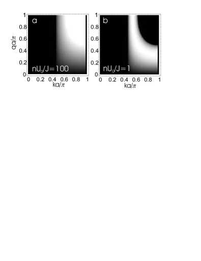
Figure 6: (a) Largest imaginary part of the eigenvalues (III.2.1) versus $k$, holding $nU_{0}=100J$, $nU_{2}=4J$. Gray scale goes from 0 to $20J$. (b) A case with a weaker nonlinearity $nU_{0}=1J$, $nU_{2}=0.04J$ Gray scale goes from 0 to $J$.

Just as we saw in the two-component case (see Fig. 4), these conditions are somewhat reversed for attractive interactions $U_{0}<0$, as then some excitations of $\omega_{1+}(q)$ are unstable whenever $ka<\pi/2$ and all the $q$ modes are unstable when $0<\cos{(ka)}<-nU_{0}/(2J)$. The dependence on the interaction coefficient $U_{0}$ is shown in Fig. 7. In these plots, we kept $U_{2}n/J=2$ constant. For $ka=0.2\pi$ (Fig. 7(a)) unstable modes occur for negative $U_{0}$, while for $ka=0.7\pi$ (Fig. 7(b)), this instability occurs for repulsive interactions $U_{0}>0$. Also, as in the two-component case, there is an additional, weaker instability in the attractive case $U_{0}<0$ with $ka>\pi/2$. This instability is driven by $\omega_{2+}(q)$ and has the same condition for instability (22) with $U_{0}$ replaced by $U_{2}$. The magnitude generally reaches $\approx\sqrt{8nU_{2}J}$ for $nU_{2}\gg J$. In the case plotted in Fig. 7(b), it has a maximum magnitude $\approx 2J$.

The equivalence of the mode energy dependence on $U_{2}$ and $U_{0}$ in Eq. (III.2.1) implies that whenever $U_{0}$ and $U_{2}$ are of opposite sign and much larger than $J$, at least one of the eigenvalues will be imaginary at any $k$. In the previous paragraph we discussed how this resulted in an instability for attractive condensates $U_{0}<0$ with polar spin-dependent scattering lengths $U_{2}>0$. Another implication of this is that polar-like condensate solutions (18) with $U_{0}>0$ are unstable for ferromagnetic spin-dependent scattering lengths $U_{2}<0$. Only when both are positive or both are negative is there a region of $k$ with dynamical stability.

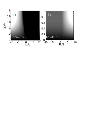
Figure 7: Imaginary part of the eigenvalues versus $nU_{0}$, for $nU_{2}=2J$ for the condensate velocities indicated. Gray scale goes from 0 to $5J$.

III.2.2 Energetic stability

Turning now to the energetic instabilities, we also obtain analytic results for the eigevalues of $\cal{M}$ and look for negative eigenvalues. We find

$$\epsilon_{1\pm}(q) =\epsilon_{q}\cos(ka)+nU_{0}\pm\sqrt{C_{q,k}^{2}+n^{2}U_{0}^{2}}$$

$$\epsilon_{2\pm}(q) =\epsilon_{q}\cos(ka)+nU_{2}\pm\sqrt{C_{q,k}^{2}+n^{2}U_{2}^{2}}.$$ (23)

For $U_{2}<U_{0}$ $\epsilon_{2-}$ drives the instability. Figure 8 plots the regions of energetic instability. There exist unstable modes for $\cos(ka)/\sin^{2}(ka)<2J/nU_{2}$. For small velocities, $ka\ll 1$, this condition is approximately equal to $\hbar k/m^{*}>\sqrt{nU_{2}/m^{*}}$, where $m^{*}=\hbar^{2}/(2Ja^{2})$ is the effective mass of a noninteracting BEC. This energetic instability threshold demonstrates the Landau criterion that the velocity becomes larger than the speed of sound (of spin waves) $a\sqrt{2JnU_{2}}/\hbar=\sqrt{nU_{2}/m^{*}}$. For $U_{2}>U_{0}$ the instability driven by $\epsilon_{1-}$ and the condition is the same, but replacing $U_{2}\rightarrow U_{0}$. When $U_{0}$ becomes negative, there is an additional instability, as shown in Fig. 8(b).

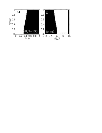
Figure 8: (a) Energetic stability (white) and instability (black) regions for $nU_{0}=100J$, $nU_{2}=4J$. (b) Dependence of the energetic stability of interaction coefficient $nU_{0}$, keeping $nU_{2}=2J$. The behavior remains qualitatively the same for non-zero $ka<\pi/2$, but with the instability region extending into the $U_{0}>0$ region.

III.3 Stability in the ferromagnetic case

III.3.1 Dynamical stability

In the ferromagnetic case (that is energetically favored for $U_{2}<0$) we consider uniform spin profiles for which the magnitude of the spin is maximized, $|\langle{\bf F}\rangle|=1$, which minimizes the mean field energy (III.1). We again assume no magnetic Zeeman shifts $\delta_{+}=\delta_{-}=0$. As in analogous states for superfluid liquid helium-3 VOL90 , the rotations of the spinor axes can be used to couple physically distinguishable ground states. Here all the degenerate states are related by spatial rotations of the atomic spin axes and we may parametrize the spin wavefunction as

$$\begin{pmatrix}\zeta_{+}\\ \zeta_{0}\\ \zeta_{-}\end{pmatrix}=e^{i\phi}\begin{pmatrix}e^{-i\alpha}\cos^{2}{(\beta/2)}\\ \sin{(\beta)}/\sqrt{2}\\ e^{i\alpha}\sin^{2}{(\beta/2)}\end{pmatrix}\,,$$ (24)

where $\alpha,\beta,\phi$ are the Euler angles. The solution (17) with Eq. (24) has a chemical potential $\mu=-2J\cos(ka)+(U_{0}+U_{2})n$ for any chosen ground state in Eq. (24). The simplest form of the Bogoliubov-de Gennes matrix $\sigma\cal{M}$ may be obtained by choosing $\beta=\alpha=\phi=0$ and substituting Eq. (24) into Eq. (38) in Appendix A.

The mode energies are found to be:

$$\omega_{1\pm}(q) =C_{q,k}\pm\epsilon_{q}\cos(ka)$$

$$\omega_{2\pm}(q) =C_{q,k}\pm\epsilon_{q}\mathrm{cos}(ka)\mp 2nU_{2}$$

$$\omega_{3\pm}(q) =C_{q,k}$$

$$\pm\sqrt{\epsilon_{q}\cos(ka)\big{[}\epsilon_{q}\cos(ka)+2n(U_{0}+U_{2})\big{]}}$$ (25)

The dynamical instabilities are driven entirely by $\omega_{3+}$ and the only difference with the polar case Eq. (III.2.1) is the replacement $U_{0}$ and $U_{2}$ individually by the sum $U_{0}+U_{2}$. This dependence can be understood from the fact that with $|\langle{\bf F}\rangle|=1$ the total nonlinearity is $\propto U_{0}+U_{2}$ and so this quantity determines the attractive or repulsive character of the condensate. Thus for $U_{0}>0$ and $|U_{2}|\ll|U_{0}|$, the instability diagrams qualitatively similar to Fig. 6.

Differences between the ferromagnetic and polar cases become clear when one examines the instability dependence on $U_{0}$. This is shown for the ferromagnetic case in Fig. 9, where we keep $nU_{2}=-2J$ constant, and should be contrasted with the polar case, Fig. 7. For $ka<\pi/2$ (the figure shows $ka=0.2\pi$), an instability occurs for $U_{0}<-U_{2}$ and increases with greater $|U_{0}|$ while for $ka>\pi/2$ (the figure shows $ka=0.7\pi$), the instability occurs for $U_{0}>-U_{2}$. An important difference from the polar case is that, for $ka>\pi/2$, there is no instability for $U_{0}<0$. In addition, the instability border occurs at $U_{0}=-U_{2}$ rather than at $U_{0}=0$. Finally, from Eq. (III.3.1), we note that a ferromagnetic BEC solution (24) with $U_{0}>0$ and a polar spin-dependent scattering length $U_{2}>0$ can be dynamically stable, in contrast to a polar solution with ferromagnetic scattering length, as discussed above.

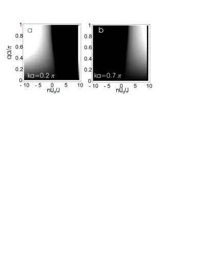
Figure 9: Imaginary part of the eigenvalues (III.2.1) versus $nU_{0}$, holding $nU_{2}=-2J$, for the two condensate velocities indicated. Gray scale goes from 0 to $5J$.

III.3.2 Energetic stability

The energy eigenvalues in the ferromagnetic case are

$$\epsilon_{1\pm}(q) = \epsilon_{q}\cos(ka)\pm C_{q,k}$$

$$\epsilon_{2\pm}(q) = \epsilon_{q}\cos(ka)-2nU_{2}\pm C_{q,k}$$

$$\epsilon_{3\pm}(q) = \epsilon_{q}\cos(ka)+n(U_{0}+U_{2})$$ (26)

$$\pm\sqrt{C_{q,k}^{2}+n^{2}(U_{0}+U_{2})^{2}}.$$

Unlike the polar case, there is one energy eigenvalue $\epsilon_{1-}$ corresponding to a pure (Doppler-shifted) kinetic energy. This gives rise to energetic instabilities for $\sin^{2}(qa/2)/\sin(qa)<\tan(ka)$, as plotted in Fig. 10(a). Though no dynamic instability exists except for much higher $k$, ferromagnetic spinor BECs are subject to this energetic instability in the presence of thermal excitation for any non-zero $k$. We note that for $ka>0.5\pi$ all $q$ modes are unstable.

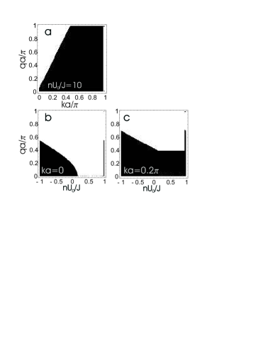
Figure 10: (a) Energetic stability regions for the ferromagnetic case with ⁸⁷Rb parameters $U_{0}=100J$, $U_{2}=-0.36J$. (b)-(c) Energetic stability versus the interaction coefficient $U_{0}$, keeping $U_{2}=-2J$.

Finally, for attractive condensates ($U_{0}+U_{2}<0$) there are additional regions of energetic instability from $\epsilon_{3-}$. Fig. 10(b-c) shows the dependence versus $U_{0}$. For $k=0$ there are unstable modes for all attractive condensate scattering length cases. A moving condensate ($ka=0.2\pi$ is shown in Fig. 10(c)), increases the region of unstable $q$ modes for attractive condensates. The band of energetic instability at low $q$ for $U_{0}>0$ in Fig. 10(c) is simply the Doppler induced energetic instability discussed above.

III.4 Effects of Zeeman splitting

When Zeeman splittings due an external magnetic field [$\delta_{\pm}$ in Eq. (III.1)] are non-zero, the symmetry of the polar and ferromagnetic solutions, Eqs. (18) and (24), breaks down and we find a new set of steady-state solutions. Here we examine these solutions and again calculate the dynamic stability of these various solutions, particularly noting how the stability varies with the linear and quadratic Zeeman shifts, which we denote, respectively, as $\tilde{\delta}=(\delta_{+}-\delta_{-})/2$ and $\bar{\delta}=(\delta_{+}+\delta_{-})/2$. The linear Zeeman shifts are $\tilde{\delta}=2g_{F}\mu_{B}B=2\big{(}(2\pi)1.4~{}\mathrm{MHz/G}\big{)}B$, where $g_{F}$ is the Land$\acute{e}$ factor, and is $-1/2$ for the ground-state $F=1$ manifold of ⁸⁷Rb and ²³Na. For Zeeman shifts substantially smaller than the hyperfine splitting, which is our interest here, the quadratic shifts $\bar{\delta}$ are typically smaller than the linear shifts and can be extracted from the Breit-Rabi formula COR77 . For alkali atoms the quadratic shift is positive, but it can generally be of either sign. The level shifts in a spin-1 BEC may also be engineered in other ways, e.g., by using off-resonant microwave fields that generate electromagnetically-induced level splittings GER06 , allowing essentially arbitrary experimentally prepared level shifts for $\tilde{\delta}$ and $\bar{\delta}$. Note that the linear Zeeman shift does not affect the energy conservation of a spin-changing collision $|m_{F}=0,m_{F}=0\rangle\leftrightarrow|m_{F}=+1,m_{F}=-1\rangle$, while the quadratic Zeeman shift does, and thus plays an important role in the stability properties.

One of the steady-state solutions in the presence of the Zeeman splitting has the chemical potential $\mu=\mu_{0}=-2J\cos{(ka)}+nU_{0}$ and reads:

$$\vec{\zeta}=e^{i\varphi}\begin{pmatrix}0\\ 1\\ 0\end{pmatrix}\,.$$ (27)

This solution forms a subset of the polar solutions (18) in the absence of the magnetic splitting, with the ${\bf d}$ pointing along the $z$ direction.

The stability is again analyzed by substituting the steady-state solution [Eq. (27)] into Eq. (38). By calculating the eigenvalues of $\sigma\cal{M}$ we obtain analytic expressions for the normal mode energies, as in Eq. (III.2.1). Here $\omega_{1\pm}(q)$ remains unchanged in the presence of the Zeeman splitting and

$$\omega_{2\pm}(q)=C_{q,k}\pm\tilde{\delta}\pm P_{q,k}$$

$$\omega_{3\pm}(q)=C_{q,k}\mp\tilde{\delta}\pm P_{q,k}$$

$$P_{q,k}=\sqrt{\big{[}\epsilon_{q}\cos(ka)+\bar{\delta}\big{]}\big{[}\epsilon_{q}\cos(ka)+2nU_{2}+\bar{\delta}\big{]}}\,,$$ (28)

The linear splitting lifts the degeneracy between $\omega_{2\pm}(q)$ and $\omega_{3\pm}(q)$ in Eq. (III.2.1) and the quadratic splitting introduces an energy gap $\bar{\delta}$ in the single-particle phonon mode spectrum $\epsilon_{q}\cos(ka)$ in $\omega_{2\pm}(q)$ and $\omega_{3\pm}(q)$.

The dynamical stability will then be governed by the sign of the square root argument of $P_{q,k}$ and is seen to be unaffected by the linear Zeeman shift. The condition for the existence of unstable modes is $-\epsilon_{q}\cos(ka)-2nU_{2}<\bar{\delta}<-\epsilon_{q}\cos(ka)$ for $U_{2}>0$, and $-\epsilon_{q}\cos(ka)<\bar{\delta}<-\epsilon_{q}\cos(ka)-2nU_{2}$ for $U_{2}<0$. If $U_{2}>0$ and $ka<\pi/2$, Eq. (III.4) predicts dynamical stability for positive quadratic shift $\bar{\delta}>0$, and instability at some $q$ for $\bar{\delta}<0$. As in previous cases, we find much larger instabilities when $ka>\pi/2$ (for $U_{0}>0$) from $\omega_{1\pm}$.

Similarly, we obtain the eigenvalues of ${\cal M}$ as in Eq. (III.2.2). Here $\epsilon_{1\pm}(q)$ is unchanged and

$$\epsilon_{2\pm}(q) =\epsilon_{q}\cos(ka)+nU_{2}+\bar{\delta}\pm\sqrt{(C_{q,k}+\tilde{\delta})^{2}+n^{2}U_{2}^{2}}$$

$$\epsilon_{3\pm}(q) =\epsilon_{q}\cos(ka)+nU_{2}+\bar{\delta}\pm\sqrt{(C_{q,k}-\tilde{\delta})^{2}+n^{2}U_{2}^{2}}\,.$$ (29)

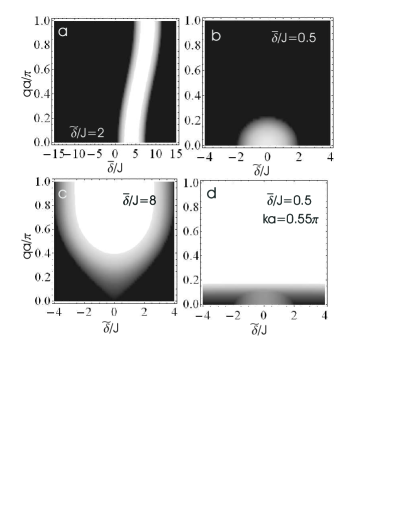
Figure 11: Largest imaginary parts of the normal mode energies for the polar-like solution Eq. (30). In all plots, $U_{0}=100J$ and $U_{2}=0.04U_{0}$ (corresponding to ²³Na). Plots are on a gray scale of 0 to $3J$. (a) Dynamic instability versus $\bar{\delta}$ for linear Zeeman shift $\tilde{\delta}=2J$ and $k=0$. (b-c) Versus linear shift $\tilde{\delta}$ for quadratic Zeeman shifts $\bar{\delta}=0.5J$ and $8J$, with $k=0$. (d) Versus $\tilde{\delta}$ with $ka=0.55\pi$.

We find another steady-state solution to the DNLSEs (III.1) with the chemical potential $\mu=\mu_{0}+\bar{\delta}$ that reads

$$\vec{\zeta}={e^{i\varphi}\over\sqrt{2}}\begin{pmatrix}e^{-i\gamma}\sqrt{1-{\tilde{\delta}/nU_{2}}}\\ 0\\ e^{i\gamma}\sqrt{1+{\tilde{\delta}/nU_{2}}}\end{pmatrix}\,.$$ (30)

This solution only exists for sufficiently small linear Zeeman shifts $|\tilde{\delta}|<|nU_{2}|$. For $\tilde{\delta}=0$, Eq. (30) coincides with the subset of solutions to Eq. (18). Although for small $\tilde{\delta}\neq 0$ the solution (30) is still close to the polar state of Eq. (18), the spin expectation value is no longer zero, $\langle{\bf F}\rangle=-\tilde{\delta}/(nU_{2}){\bf\hat{z}}$, with ${\bf d}$ restricted on the $xy$ plane and the induced $\langle{\bf F}\rangle$ pointing along the $z$ axis comment2 . At the boundary of the validity of Eq. (18), $\tilde{\delta}=\pm nU_{2}$, we obtain $\langle{\bf F}\rangle=\mp{\bf\hat{z}}$, as in a ferromagnetic state, so that Eq. (30) in fact interpolates between the polar and the ferromagnetic solutions. Moreover, we again find analytic solutions for the normal mode energies:

$$\omega_{1\pm}(q) =C_{q,k}\pm\sqrt{\epsilon_{q}\cos(ka)\big{[}\epsilon_{q}\cos(ka)+2nU_{2}-2\bar{\delta}\big{]}+\tilde{\delta}^{2}+\bar{\delta}^{2}-2nU_{2}\bar{\delta}}$$

$$\omega_{2\pm}(q) =C_{q,k}\pm\sqrt{\epsilon_{q}\cos(ka)\big{[}\epsilon_{q}\cos(ka)+n(U_{0}+U_{2})\big{]}+L_{q,k}}$$

$$\omega_{3\pm}(q) =C_{q,k}\pm\sqrt{\epsilon_{q}\cos(ka)\big{[}\epsilon_{q}\cos(ka)+n(U_{0}+U_{2})\big{]}-L_{q,k}}$$

$$L_{q,k} =\sqrt{\epsilon_{q}^{2}\cos^{2}(ka)\big{[}n^{2}(U_{0}-U_{2})^{2}+4\tilde{\delta}^{2}U_{0}/U_{2}\big{]}}\,.$$ (31)

For $U_{0},U_{2}>0$ and $ka<\pi/2$, whenever the solution (30) exists (i.e., when $|nU_{2}|\geq|\tilde{\delta}|$), the dynamical instabilities are solely driven by $\omega_{1\pm}(q)$. Moreover, under these conditions the mode $\omega_{1\pm}(q)$ is dynamically stable when Eq. (30) is energetically favorable to Eq. (27) (i.e., when $\bar{\delta}<0$). In Fig. 11 we show some stability diagrams for the parameters of ²³Na. The instability dependence on the quadratic Zeeman shift for a particular linear Zeeman shift is shown in Fig. 11(a). This diagram may be understood by noting that the mode $\omega_{1\pm}(q)$ exhibits a nonvanishing imaginary part, if

$$c_{-}<\bar{\delta}<c_{+},$$

$$c_{\pm}\equiv\epsilon_{q}\cos(ka)+nU_{2}\pm\sqrt{n^{2}U_{2}^{2}-\tilde{\delta}^{2}}\,.$$ (32)

This forms an instability stripe with a width $2(n^{2}U_{2}^{2}-\tilde{\delta}^{2})^{1/2}$ in Fig. 11(a) and for larger values of $\bar{\delta}$ the system stabilizes again. We observe the stripe position shift in $\bar{\delta}$ by $4J$ from the $qa=0$ to $qa=\pi$. We also calculated the energetic stability of Eq. (30) and found that in Fig. 11(a) the region to the left of the stripe is energetically stable, while the entire region to the right of the stripe (i.e., large $\bar{\delta}$) is energetically unstable.

While not obvious in Fig. 11(a) there is a small region of stability for positive $\bar{\delta}$. This is seen more easily by plotting the instability versus the linear Zeeman shift. In Figs. 11(b-d) we plot this for the entire range of validity of Eq. (30) ($|\tilde{\delta}|\leq|nU_{2}|$) for various $\bar{\delta}$. For small quadratic Zeeman shift, there exists a range of linear Zeeman shifts which stabilize the system, as it approaches the ferromagnetic state. For larger quadratic shifts this range shrinks, until eventually the system is unstable at all possible $\tilde{\delta}$, as in Fig. 11(b).

The effect of larger $k$ is generally simply to stretch the region of instability to larger ranges of $q$ for each case, as the effect of the $\epsilon_{q}$ shift in Eq. (32) vanishes. For $ka>0.5\pi$ (with $U_{0}>0$) the usual, and much larger, instability for large $k$, seen in previous cases, dominates the stability diagram. Such a case is plotted in Fig. 11(d).

In the absence of the Zeeman splitting the polar state (18) is always dynamically unstable for $U_{2}<0$. For the state (30), even close to the polar state, this is no longer the case. For $U_{0}>0$ and $U_{2}<0$, Eq. (32) represents the entire unstable region, provided that $4\tilde{\delta}^{2}|U_{0}/U_{2}|\leq n^{2}(U_{0}-U_{2})^{2}$ and $|U_{0}|>|U_{2}|$.

In the presence of the Zeeman splitting the ferromagnetic state (24) is modified to

$$\vec{\zeta}=e^{i\phi}\begin{pmatrix}1\\ 0\\ 0\end{pmatrix}\,,$$ (33)

with the chemical potential $\mu=\mu_{0}+nU_{2}+\delta_{+}$, or to an analogous ferromagnetic state with $(\zeta_{+},\delta_{+})$ interchanged with $(\zeta_{-},\delta_{-})$. Although Eq. (33) is a steady-state solution to the DNLSEs (III.1) for any values of $\tilde{\delta}$, we also find that the solution (30) has the limit Eq. (33) at the boundary of the validity region $\tilde{\delta}=-nU_{2}$. At the other limit of the validity of Eq. (30) (at $\tilde{\delta}=nU_{2}$) we recover the other ferromagnetic state, defined by $(\zeta_{-},\delta_{-})$. Moreover, the solution (33) is energetically favorable to Eq. (27) when $nU_{2}/2+\delta_{+}<0$ and to Eq. (30) when $nU_{2}/2+\tilde{\delta}<0$.

We find that the normal mode energies and the eigenvalues of ${\cal M}$ corresponding to Eq. (33) are obtained from the non-Zeeman shifted mode frequencies, Eqs. (III.3.1) and (III.3.2), by shifting the single-particle excitation energies: $\epsilon_{q}\cos(ka)\rightarrow\epsilon_{q}\cos(ka)-\delta_{+}$ in $\omega_{1\pm}(q)$ and $\epsilon_{1\pm}(q)$; and $\epsilon_{q}\cos(ka)\rightarrow\epsilon_{q}\cos(ka)-2\tilde{\delta}$ in $\omega_{2\pm}(q)$ and $\epsilon_{2\pm}(q)$. The energies $\omega_{3\pm}(q)$ and $\epsilon_{3\pm}(q)$ are unchanged. Because it is $\omega_{3\pm}$ which drives the dynamical instability, the stability diagram is unchanged from that of Eq. (III.3.1).

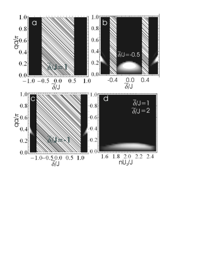
Figure 12: Largest imaginary parts of the normal mode energies for the solution Eq. (III.4). In all plots, $nU_{0}=100J$. Hatched areas represent regions where the condensate solution is not valid. (a)-(c) Dynamic instability versus linear Zeeman shift and $q$ for $U_{2}=-0.0036U_{0}$ (corresponding to ⁸⁷Rb). Gray scale runs from (a) 0 to $0.3J$, (b) 0 to $0.3J$, (c) 0 to $0.2J$. In (a) we emphasize that there is a range of $\tilde{\delta}$, on each side of the instability region, stable for all $q$. (d) Dynamic instability versus spin-dependent scattering length $U_{2}$ for $\tilde{\delta}=2J$ and $\bar{\delta}=J$. Gray scale from 0 to $0.2J$.

We find an additional ferromagnetic-like steady-state solution to the DNLSEs (III.1) with $\mu=\mu_{0}+nU_{2}+(\bar{\delta}^{2}-\tilde{\delta}^{2})/2\bar{\delta}$, that reads

$$\zeta_{\pm} =e^{i\gamma_{\pm}}\delta_{\mp}\sqrt{{2nU_{2}\bar{\delta}+\bar{\delta}^{2}-\tilde{\delta}^{2}\over 8nU_{2}\bar{\delta}^{3}}},$$

$$\zeta_{0} =e^{i(\gamma_{+}+\gamma_{-})/2}\sqrt{1-|\zeta_{+}|^{2}-|\zeta_{-}|^{2}}\,.$$ (34)

This solution only exists if the expressions inside the square roots of Eq. (III.4) are positive, i.e.,

$$0\leq{2nU_{2}\bar{\delta}+\bar{\delta}^{2}-\tilde{\delta}^{2}\over 8nU_{2}\bar{\delta}^{3}}\leq{1\over 2(\tilde{\delta}^{2}+\bar{\delta}^{2})}\,.$$ (35)

This condition gives rise to a ranges of validity for $U_{2}$ in terms of two parameters $\beta_{-}=(\tilde{\delta}^{2}-\bar{\delta}^{2})/2\bar{\delta}$ and $\beta_{+}=(\tilde{\delta}^{2}+\bar{\delta}^{2})/2\bar{\delta}$. In the most common case that the linear Zeeman shift is larger in magnitude ($|\tilde{\delta}|>|\bar{\delta}|$) these inequalities give a finite range: $\beta_{-}<nU_{2}<\beta_{+}$ for $\bar{\delta}>0$ and $\beta_{+}<nU_{2}<\beta_{-}$ for $\bar{\delta}<0$.

If $|\tilde{\delta}|<|\bar{\delta}|$, the inequalities change direction, giving instead an intermediate range of $U_{2}$ where (III.4) is not valid. In particular, the requirement for validity for $\bar{\delta}>0$ is $nU_{2}<\beta_{-}$ or $nU_{2}>\beta_{+}$, while for $\bar{\delta}<0$ it is $nU_{2}<\beta_{+}$ or $nU_{2}>\beta_{-}$.

At the lower limit of Eq. (35) ($nU_{2}=\beta_{-}$) the solution (III.4) coincides with the polar solution (27) with $\langle{\bf F}\rangle=0$, while at upper limit ($nU_{2}=\beta_{+}$) it equals Eq. (30). In general, the spin for the solution (III.4) is non-vanishing

$$|\langle{\bf F}\rangle|^{2}={2\bar{\delta}^{2}(\tilde{\delta}^{2}+2n^{2}U_{2}^{2})-\bar{\delta}^{4}-\tilde{\delta}^{4}\over 4\bar{\delta}^{2}n^{2}U_{2}^{2}}\,.$$ (36)

This condensate solution (III.4) is energetically favorable to (33) for positive quadratic shifts $\bar{\delta}>0$, the opposite relationship of solution (30) to (27).

We computed the dynamical and energetic stability of this solution. Figures 12(a)-(c) show the dynamical instability strengths as a function linear Zeeman shift for several quadratic shifts and Rb-87 scattering length ($U_{2}=-0.0036U_{0}$). The hatched areas and all $|\tilde{\delta}|$ larger than the range of these plots are regions where the condensate solution (III.4) is not valid. For $\bar{\delta}>0$ (Fig. 12(a)) we see the valid regions where the solution exists are dynamically stable. For $\bar{\delta}<0$ (Figs. 12(b)-(c)) there are always some unstable modes $q$. However note the interesting behavior that for large $|\tilde{\delta}|$, there exist only small bands of unstable $q$ and weak instability (note the range of the plots in the caption). The system is energetically unstable for $q$ in the regions overlapping and below the small dynamical instability bands.

In Fig. 12(d) we plot the instability strength versus $U_{2}$ over its range of validity, which in this case is $1.5J<nU_{2}<2.5J$. Here we see a weak band of instability for low $q$ in the range of $U_{2}$ where the solution exists.

IV Experimental considerations

In the experimental realizations of optical lattice systems, ultra-cold atoms have been trapped in a combined optical lattice and a harmonic trap. The transport properties may then be studied by suddenly displacing the harmonic trap, e.g., by using a magnetic field gradient. This excites dipolar oscillations of atoms along the lattice direction with the maximum velocity proportional to the harmonic trap displacement BUR01 ; FER05 . The other alternative is to use a moving-standing wave, so that the atoms are trapped close to the harmonic trap minimum and experience a moving optical lattice potential FAL04 ; SAR05 . The advantage of the latter technique is that the velocity of the atoms with respect to the lattice is constant. In such transport experiments the dynamical instabilities may typically be observed on much shorter time scales than the energetic ones and the rate of the energetic instability to have an observable effect can be controlled by increasing the size of the thermal atom cloud SAR05 .

A two-component ultra-cold ⁸⁷Rb vapor has also been trapped in a spin-dependent lattice using two counter-propagating laser beams with linear polarizations MAN03 . The two species experience different $\sigma_{+}$ and $\sigma_{-}$ polarized optical lattices where the separation between the lattice potentials can be controlled by changing the angle between the linear polarization vectors.

The techniques developed for investigating dynamical and energetic instabilities in a single component case could be adapted to our proposed two-component BEC studies. A spin-dependent lattice potential may be used to control the value of the intraspecies interaction strength $U_{12}$ by modifying the spatial overlap integral between the lattice site wavefunctions of the two species. Moreover, the various intra- and inter-species scattering lengths and the two species Feshbach resonances KOK07 in two-component BEC systems make them a very rich area for experimental exploration. In addition to the two-component ⁸⁷Rb vapor MAN03 , two-component BECs have been experimentally realized in optical lattices using a ⁴¹K–⁸⁷Rb mixture CAT07 .

Different superfluid velocities for the two species can be realized in such a system by moving the two lattice potentials at different speed. The disadvantage of this scheme is that it would make the intraspecies interaction strength $U_{12}$ time-dependent. Displacing the harmonic trapping potentials of the two BECs different distances, in such a way that at the end the traps are perfectly overlapping, could be used to realize two BECs undergoing dipolar oscillations in phase with different amplitudes. Perhaps the easiest method to measure the reversed phase separation instability in a two-species BEC, as discussed in Section II.2.3 and Appendix B, is to move the lattice potentials of the both species at the same speed and to use light-stimulated coherent Bragg diffraction KOZ99 to change the velocity of one of the BECs. For sufficiently small velocities of the Bragg diffracted BEC, the atomic clouds of the two BECs overlap long enough for the dynamical instabilities to have an observable effect.

Atomic ⁸⁷Rb spin-1 gases have also been loaded to optical lattices WID05 . In such a system the linear and quadratic Zeeman shifts could be modified, e.g., by using off-resonant microwave field-induced level shifts GER06 . This would allow the studies of the stability properties of different steady-state solutions presented here.

V Conclusions

We studied the transport properties of two-component and spinor atomic BECs in optical lattices using the discrete nonlinear Schrodinger equations, obtained in the tight-binding approximation to the lattice system. The classical GP theory is valid in optical lattices at low temperatures if the effective 1D nonlinearity is not too large, the atom number not too small, or the lattice potential not too deep ISE05 . In particular, we studied both the dynamical and energetic stability of homogenous Bloch wave solutions to the DNLSEs for the condensates by analyzing the linearized perturbations around the carrier wave. In the case of the dynamical instabilities this involved finding the eigenvalues (normal mode energies) of the corresponding Bogoliubov-de Gennes equations [the matrix $\sigma{\cal M}$ in Eq. (5)] and in the case of energetic instabilities finding the eigenvalues of the second order perturbations in the energy functional (the matrix ${\cal M}$). Our steady-state Bloch wave ansatz allowed for magnetic Zeeman level shifts and even for two different velocities of the condensates in the two-component case. Our study discusses a large number of cases and points out how the spin degree of freedom can affect the stability properties.

In the two-component case we analyzed and fully characterized the dynamical and energetic instabilities for the general case of the two BECs exhibiting arbitrary hopping amplitudes, interaction strengths, superfluid velocities, and spatial overlap. Simple analytic expressions for the normal mode energies [Eq. (6)] and the dynamical stability criteria were obtained in the important case of the two BECs having the same atom current (even when the velocities may differ).

For the case that $\cos(k_{1}a)$ and $\cos(k_{2}a)$ exhibit equal sign for the two BEC carrier wavenumbers $k_{1},k_{2}$ (see Sec. II.2.2), we found that the instability diagram contains contributions from: (1) the high velocity instability, determined by Eq. (12), (which is analogous to that of a single-component BEC in a lattice), and (2) a weaker phase-separation instability [Eq. (13)], which occurs when $U_{12}^{2}>U_{11}U_{22}$. However, as shown in Appendix B and in Sec. II.2.3, an interesting case arises when one allows different condensate velocities of the two-components, so that $\cos(k_{1}a)$ and $\cos(k_{2}a)$ exhibit different sign (the effective masses of the two components exhibit different signs). Firstly, the high velocity instability conditions (which depends on the velocities, hopping amplitudes, atom numbers, and interaction strengths of the two BECs) indicate that the presence of the other condensate component can stabilize the superfluid flow of an otherwise unstable condensate (that exceeds the critical velocity of a single-component BEC). Secondly, the phase separation stability criteria can be reversed for particular sets of parameters and the entire dynamically stable regime exists for $U_{12}^{2}>U_{11}U_{22}$; see Appendix B and Figs. 3(c-d).

For the spin-1 BEC case, we also obtained analytic expressions for the dynamical and energetic instabilities in several cases of interest. In the absence of the Zeeman level shifts the normal mode energies in the polar and ferromagnetic ground state manifolds are simplified and the two cases differ when $U_{0}<0$ and for relatively large spin-dependent interactions $|U_{2}|\sim|U_{0}|$. In particular, the polar case tends to exhibit more regions of instability as $U_{0}$ and $U_{2}$ separately contribute [see Eq. (III.2.1)], while in the ferromagnetic case, it is the sum $U_{0}+U_{2}$ which is important; see Eq. (III.3.1). This allows for dynamical stability of ferromagnetic solutions for $U_{0}<0$, and even for polar spin-dependent scattering lengths ($U_{2}>0$). Also, we found that, unlike the polar case, the ferromagnetic solution will have some energetic instability for any finite BEC velocity due to the existence of a pure kinetic energy eigenvalue $\epsilon_{1\pm}$ [Eq. (III.3.2)].

In the presence of the linear and quadratic Zeeman level shifts we find a new set of steady-state Bloch wave solutions, describing the superfluid flow in spin-1 BECs. While the polar-like solution (27) and the ferromagnetic-like solution (33) form subsets of the corresponding solutions in the absence of the Zeeman splitting, this is not the case for the steady-state solutions (30) and (III.4). The solution (30) exhibits a nonvanishing spin vector $\langle{\bf F}\rangle$ pointing along the magnetic field and interpolates between the polar and the ferromagnetic solutions. The solution (III.4) only exists in the presence of sufficiently large Zeeman shifts and in this sense represents an entirely novel state.

We analyzed the stability conditions for all spin-1 Bloch wave states. For condensate solutions unique to the presence of Zeeman shift, Eqs. (30) and (III.4), the stability diagrams were presented in Figs. 11 and 12, respectively. For the parameters of ²³Na at low velocities we found the solution Eq. (30) to be dynamically stable for negative quadratic shifts. Even for positive quadratic shift, a sufficiently large linear shift can stabilize it. Moreover, the solution (30) can be stable for ferromagnetic scattering coefficients ($U_{2}<0$), even close to the polar state. For the parameters of ⁸⁷Rb the solution Eq. (III.4) can be energetically and dynamically stable for positive quadratic Zeeman shifts and sufficiently large linear Zeeman shifts.

The phenomena discussed in this paper should be applicable to current and future experiments with multiple-component BECs in optical lattices, and we discussed some of the important considerations for the experimental realization. We concentrated on the stability studies of moving Bloch wave solutions in the lattice. An interesting theoretical extension of this work is to consider inhomogenous condensate solutions, such as soliton-like structures in spinor BECs DAB07 . One could also investigate the effect of spin-dependent lattice potentials with spatially inhomogeneous profiles for the hopping amplitude, for instance dimerization, along the lattice RUO02 .

Appendix A Bogoliubov-de Gennes matrices

In the two-component case, the Bogoliubov-de Gennes equation, upon substitution of the the ansatz (4) into (2), we get (5) with:

$$\cal{M}=\left(\begin{array}[]{cccc}K_{1+}+\bar{U}_{1}&-\bar{U_{1}}&\bar{U}_{12}&-\bar{U}_{12}\\ -\bar{U}_{1}&K_{1-}+\bar{U}_{1}&-\bar{U}_{12}&\bar{U}_{12}\\ \bar{U}_{12}&-\bar{U}_{12}&K_{2+}+\bar{U}_{2}&-\bar{U}_{2}\\ -\bar{U}_{12}&\bar{U}_{12}&-\bar{U}_{2}&K_{2-}+\bar{U}_{2}\\ \end{array}\right)$$ (37)

where $K_{j\pm}=(4J_{j}/\hbar)\sin^{2}(qa/2)\cos(k_{j}a)\pm(2J_{j}/\hbar)\sin(qa)\sin(k_{j}a)$, $\bar{U}_{j}=U_{j}n_{j}/\hbar$, and $\bar{U}_{12}=U_{12}\sqrt{n_{1}n_{2}}/\hbar$.

In the general spinor case, we obtain the $\cal{M}$ for the spinor wavefunction and the Bogoliubov expansion (4), into the DNLSEs (III.1):

$$\cal{M}=\left(\begin{array}[]{cccccc}M_{-}^{(+)}&w_{++}&f_{0+}^{0-}&w_{0+}&r_{-+}&g_{-+}^{0}\\ (w_{++})^{*}&M_{+}^{(+)}&(w_{0+})^{*}&(f_{0+}^{0-})^{*}&(g_{-+}^{0})^{*}&(r_{-+})^{*}\\ (f_{0+}^{0-})^{*}&w_{0+}&M_{-}^{(0)}&h^{-+}_{0}&(f_{0-}^{0+})^{*}&w_{0-}\\ (w_{0+})^{*}&f_{0+}^{0-}&(h^{-+}_{0})^{*}&M_{+}^{(0)}&(w_{0-})^{*}&f_{0-}^{0+}\\ (r_{-+})^{*}&g_{-+}^{0}&f_{0-}^{0+}&w_{0-}&M_{-}^{(-)}&w_{--}\\ (g_{-+}^{0})^{*}&r_{-+}&(w_{0-})^{*}&(f_{0-}^{0+})^{*}&(w_{--})^{*}&M_{+}^{(-)}\\ \end{array}\right)$$ (38)

$$M_{\pm}^{(+)} =K_{\pm}+\bar{U}(1+|\zeta_{+}|^{2})+\tilde{U}(2|\zeta_{+}|^{2}+|\zeta_{0}|^{2}-|\zeta_{-}|^{2})+\delta_{+},$$ (39)

$$M_{\pm}^{(0)} =K_{\pm}+\bar{U}(1+|\zeta_{0}|^{2})+\tilde{U}(|\zeta_{+}|^{2}+|\zeta_{-}|^{2}),$$ (40)

$$M_{\pm}^{(-)} =K_{\pm}+\bar{U}(1+|\zeta_{-}|^{2})+\tilde{U}(-|\zeta_{+}|^{2}+|\zeta_{0}|^{2}+2|\zeta_{-}|^{2})+\delta_{-},$$ (41)

$$f_{kl}^{mn} =(\bar{U}+\tilde{U})\zeta_{k}^{*}\zeta_{l}+2\tilde{U}\zeta_{m}\zeta_{n}^{*},$$ (42)

$$g_{kl}^{m} =(\tilde{U}-\bar{U})\zeta_{k}\zeta_{l}-\tilde{U}\zeta_{m}^{2},$$ (43)

$$h^{lm}_{k} =-\bar{U}\zeta_{k}^{2}-2\tilde{U}\zeta_{l}\zeta_{m},$$ (44)

$$w_{kl} =-(\bar{U}+\tilde{U})\zeta_{k}\zeta_{l},$$ (45)

$$r_{kl} =(\bar{U}-\tilde{U})\zeta_{k}^{*}\zeta_{l}\,.$$ (46)

Here $\bar{U}=nU_{0}/\hbar$, $\tilde{U}=nU_{2}/\hbar$, and

$$K_{\pm}=-2(J/\hbar)\cos(ka)+(4J/\hbar)\sin^{2}(qa/2)\cos(ka)\pm(2J/\hbar)\sin(qa)\sin(ka)-\mu\,.$$ (47)

Appendix B Dynamical stability for $k_{1}a>\pi/2$, $k_{2}a<\pi/2$

In this section we analyze the dynamical stability of the two-component BEC system with equal atom currents $J_{1}\sin(k_{1}a)=J_{2}\sin(k_{2}a)$, when $\cos{(k_{1}a)}$ and $\cos{(k_{2}a)}$ exhibit different signs. Setting the atom currents to be equal allows us to obtain simple analytic expressions for the stability conditions. The different signs of $\cos{(k_{1}a)}$ and $\cos{(k_{2}a)}$ represent the situation where the velocities of the two BECs are located on the opposite sides of the deflection point in the ideal, single-particle BEC excitation spectrum (8) (the effective masses of the two components exhibit different signs). Without loss of generality we assume in the following that $\cos{(k_{1}a)}<0$ and $\cos{(k_{2}a)}>0$. The situation where when $\cos{(k_{1}a)}$ and $\cos{(k_{2}a)}$ have the equal sign is covered in Sec II.2.

The analytic result for the normal mode energies is given by Eq. (6). Similarly to the case when $\cos{(k_{1}a)}$ and $\cos{(k_{2}a)}$ have the same sign, the system is always dynamically unstable if $\omega_{1,q}^{2}+\omega_{2,q}^{2}<0$ and we have the same condition as in Eq. (12):

$$D_{11}+D_{22}<0\,,$$ (48)

where $D_{ij}$ is defined in Eq. (11). Since $k_{1}a>\pi/2$ and $k_{2}a<\pi/2$ and $J_{1},J_{2}>0$, the inequality may even be satisfied for some values for which $U_{11},U_{22}>0$. In this case only one of the BECs reaches the (single-component) critical velocity $ka=\pi/2$, destabilizing the entire two-component BEC system.

Next we assume $\omega_{1,q}^{2}+\omega_{2,q}^{2}\geq 0$ and find the additional unstable regions of the parameter space. When $\cos{(k_{1}a)}$ and $\cos{(k_{2}a)}$ have different signs, the expression inside the inner square root in Eq. (6) may become negative, resulting in a dynamical instability. In particular, this happens at least for some values of $q$, if

$$U_{12}^{2}>\xi_{1}\,,$$ (49)

where

$$\xi_{1}=-{(D_{11}-D_{22})^{2}\over 4n_{1}n_{2}J_{1}\cos{(k_{1}a)}J_{2}\cos{(k_{2}a)}}\,,$$ (50)

where $D_{ij}$ is defined in Eq. (11).

Also the expression inside the outer square root may become negative. If

$$n_{1}U_{11}<n_{2}U_{22}\,{\rm min}\left(\left|{J_{2}\cos(k_{2}a)\over J_{1}\cos(k_{1}a)}\right|,\left|{J_{1}\cos(k_{1}a)\over J_{2}\cos(k_{2}a)}\right|\right)\,,$$ (51)

this happens at least for some values of $q$, if $U_{11}U_{22}>U_{12}^{2}$. Combining this with Eq. (49) we find that the system is stable for the values of $U_{11}$ that satisfy Eq. (51), if

$$U_{11}U_{22}<U_{12}^{2}<\xi_{1}\,.$$ (52)

Similarly, for the values of $U_{11}$ satisfying

$$n_{1}U_{11}>n_{2}U_{22}\left|{J_{1}\cos(k_{1}a)\over J_{2}\cos(k_{2}a)}\right|-4J_{1}\cos(k_{1}a)$$

$$n_{1}U_{11}<n_{2}U_{22}\left|{J_{2}\cos(k_{2}a)\over J_{1}\cos(k_{1}a)}\right|\,,$$ (53)

we find that a dynamically stable system exists if

$$\xi_{2}<U_{12}^{2}<\xi_{1}\,,$$ (54)

where

$$\xi_{2}= U_{11}U_{22}+4J_{1}\cos{(k_{1}a)}J_{2}\cos{(k_{2}a)}/(n_{1}n_{2})$$

$$+2[J_{1}\cos(k_{1}a)U_{22}/n_{1}+J_{2}\cos(k_{2}a)U_{11}/n_{2}]\,.$$ (55)

When $U_{11}$ satisfies Eq. (53), $\xi_{2}$ is always larger than $U_{11}U_{22}$ and for the dynamically stable region we have $U_{11}U_{22}<\xi_{2}<U_{12}^{2}<\xi_{1}$. If $\xi_{2}>\xi_{1}$, no stable region exists.

Note that the entire stable region in both Eqs. (52) and (54) correspond to the values of the nonlinearities satisfying $U_{11}U_{22}<U_{12}^{2}$ that is normally associated with the dynamically unstable phase separation condition.

The two-component system is therefore dynamically stable if $D_{11}+D_{22}>0$ and $U_{12}$ satisfies either Eq. (52) or Eq. (54), for $U_{11}$ defined by Eq. (51) or Eq. (53), respectively. Interestingly, we find a regime where the other condensate component can stabilize the superfluid flow of an otherwise unstable condensate. The inequalities (51) or (53) can be satisfied for $U_{11},U_{22}>0$ when the component $\psi_{1}$ exceeds the critical velocity of the single-component BEC, with $k_{1}a>\pi/2$, so that $\omega_{1,q}^{2}<0$ in Eq. (7). The two-component BEC dynamics, nevertheless, is stable if $U_{12}$ satisfies either Eq. (52) or Eq. (54), respectively.

Note also that we may have, e.g., $U_{11}<0$, $U_{22}>0$, but $\omega_{1,q}^{2}+\omega_{2,q}^{2}>0$ (i.e., $D_{11}+D_{22}>0$). Such a two-component system can be dynamically stable since $U_{12}^{2}>U_{11}U_{22}$.

References

- (1) B.P. Anderson and M.A. Kasevich, Science 282, 1686 (1998).
- (2) S. Burger, F.S. Cataliotti, C. Fort, F. Minardi, M. Inguscio, M.L. Chiofalo, and M.P. Tosi, Phys. Rev. Lett. 86, 4447 (2001).
- (3) O. Morsch, J.H. Müller, M. Cristiani, D. Ciampini, and E. Arimondo, Phys. Rev. Lett. 87, 140402 (2001).
- (4) F.S. Cataliotti, S. Burger, C. Fort, P. Maddaloni, F. Minardi, A. Trombettoni, A. Smerzi, and M. Inguscio, Science 293, 843 (2001).
- (5) F.S. Cataliotti, L. Fallani, F. Ferlaino, C. Fort, P. Maddaloni, and M. Inguscio, New J. Phys. 5, 71 (2003).
- (6) M. Cristiani, O. Morsch, M. Malossi, M. Jona-Lasinio, M. Anderlini, E. Courtade, and E. Arimondo, Opt. Express 12, 4 (2004).
- (7) L. Fallani, L. De Sarlo, J.E. Lye, M. Modugno, R. Saers, C. Fort, and M. Inguscio, Phys. Rev. Lett. 93, 140406 (2004).
- (8) L. De Sarlo, L. Fallani, J.E. Lye, M. Modugno, R. Saers, C. Fort, and M. Inguscio, Phys. Rev. A72, 013603 (2005).
- (9) C.D. Fertig, K.M. O’Hara, J.H. Huckans, S.L. Rolston, W.D. Phillips, and J.V. Porto, Phys. Rev. Lett. 94, 120403 (2005).
- (10) A.K. Tuchman, W. Li, H. Chien, S. Dettmer, and M.A. Kasevich, New J. Phys. 8, 311 (2006).
- (11) A.J. Ferris, M.J. Davis, R.W. Geursen, P.B. Blakie, and A.C. Wilson, e-print arXiv:0706.2744.
- (12) B. Wu and Q. Niu, Phys. Rev. A64, 061603 (2001).
- (13) A. Smerzi, A. Trombettoni, P.G. Kevrekidis, and A.R. Bishop, Phys. Rev. Lett. 89, 170402 (2002).
- (14) B. Wu and Q. Niu, New J. Phys. 5, 104 (2003).
- (15) Y. Zheng, M. Kostrun, and J. Javanainen, Phys. Rev. Lett. 93, 230401 (2004).
- (16) M. Modugno, C. Tozzo, and F. Dalfovo, Phys. Rev. A70, 043625 (2004).
- (17) A. Polkovnikov and D.-W. Wang, Phys. Rev. Lett. 93, 070401 (2004).
- (18) J. Ruostekoski and L. Isella, Phys. Rev. Lett. 95, 110403 (2005).
- (19) J. Gea-Banacloche, A.M. Rey, G. Pupillo, C.J. Williams, and C.W. Clark , Phys. Rev. A 73, 013605 (2006).
- (20) Note also that, at least in deep lattices, the dissipative atom current may manifest itself in the formation of phase slips, as studied by A. Polkovnikov, E. Altman, E. Demler, B. Halperin, and M.D. Lukin, Phys. Rev. A71, 063613 (2005).
- (21) J.M. Vogels, R.S. Freeland, C.C. Tsai, B.J. Verhaar, and D. J. Heinzen, Phys. Rev. A 61 043407 (2000).
- (22) D.S. Hall, M.R. Matthews, J.R. Ensher, C.E. Wieman, and E.A. Cornell, Phys. Rev. Lett. 81, 1539 (1998).
- (23) Z. Dutton, M. Budde, C. Slowe, and L.V. Hau, Science 293, 663 (2001).
- (24) H. J. Lewandowski, D. M. Harber, D. L. Whitaker, and E. A. Cornell, 88, 070403 (2002).
- (25) T. Nikuni and J. E. Williams, J. of Low Temp. Phys. 133, 323 (2003).
- (26) G. Modugno, M. Modugno, F. Riboli, G. Roati, and M. Inguscio, Phys. Rev. Lett. 89, 190404 (2002).
- (27) A. Sorensen, L.-M. Duan, J. I. Cirac, and P. Zoller, Nature 409 63 (2001).
- (28) J. Ruostekoski and J.R. Anglin, Phys. Rev. Lett. 86, 3934 (2001).
- (29) Th. Busch and J. R. Anglin, Phys. Rev. Lett. 87, 010401 (2001).
- (30) C.M. Savage and J. Ruostekoski, Phys. Rev. Lett. 91, 010403 (2003).
- (31) O. Mandel, M. Greiner, A. Widera, T. Rom, T.W. Hänsch, and I. Bloch, Nature 425, 937 (2003).
- (32) J. Catani, L. De Sarlo, G. Barontini, F. Minardi, and M. Inguscio, arXiv:0706.2781.
- (33) J. Stenger, S. Inouye, D.M. Stamper-Kurn, H.J. Miesner, A.P. Chikkatur, and W. Ketterle, Nature (London) 396, 345 (1998).
- (34) H.-J. Miesner, D.M. Stamper-Kurn, J. Stenger, S. Inouye, A.P. Chikkatur, and W. Ketterle, Phys. Rev. Lett. 82, 2228 (1999).
- (35) A.E. Leanhardt, Y. Shin, D. Kielpinski, D.E. Pritchard, and W. Ketterle, Phys. Rev. Lett. 90, 140403 (2003).
- (36) F. Zhou, Int. J. Mod. Phys. B 17, 2643 (2003).
- (37) J. Ruostekoski and J.R. Anglin, Phys. Rev. Lett. 91 190402 (2003).
- (38) E.J. Mueller, Phys. Rev. A69, 033606 (2004).
- (39) J.W. Reijnders, F.J.M. van Lankvelt, K. Schoutens, N. Read, Phys. Rev. A69, 023612 (2004).
- (40) H. Schmaljohann, M. Erhard, J. Kronjäger, M. Kottke, S. van Staa, L. Cacciapuoti, J.J. Arlt, K. Bongs, and K. Sengstock, Phys. Rev. Lett. 92, 040402 (2004).
- (41) M.-S. Chang, C.D. Hamley, M.D. Barrett, J.A. Sauer, K.M. Fortier, W. Zhang, L. You, and M.S. Chapman, Phys. Rev. Lett. 92, 140403 (2004).
- (42) J. Kronjäger, et al., Phys. Rev. A 72, 063619 (2005).
- (43) A.T. Black, E. Gomez, L. D. Turner, S. Jung, and P. D. Lett, arXiv:0704.0925.
- (44) A. Widera, F. Gerbier, S. Fölling, T. Gericke, O. Mandel, and I. Bloch, Phys. Rev. Lett. 95, 190405 (2005).
- (45) M. Vengalattore, et al., Phys. Rev. Lett. 98, 200801 (2007).
- (46) S. Hooley and K.A. Benedict, e-print cond-mat/0610364.
- (47) B. J. Da̧browska-Wüster, E. A. Ostrovskaya, T. J. Alexander, and Y. S. Kivshar, Phys. Rev. A75, 023617 (2007).
- (48) D.M. Harber, H.J. Lewandowski, J.M. McGuirk, and E.A. Cornell, Phys. Rev. A66, 053616 (2002).
- (49) D. Jaksch, C. Bruder, J.I. Cirac, C.W. Gardiner, and P. Zoller, Phys. Rev. Lett. 81, 3108 (1998).
- (50) C. Pethick and H. Smith, Bose-Einstein condensation in dilute gases (Cambridge University Press, Cambridge, 2002).
- (51) A. Widera, F. Gerbier, S. Fölling, T. Gericke, O. Mandel, and I. Bloch, New J. of Phys. 8, 152 (2006).
- (52) In principle, an external magnetic field may also induce a different hopping amplitude for different internal levels, but in the present study we ignore such effects.
- (53) D. Vollhardt and P. Wölfle,The Superfluid Phases of Helium 3 (Taylor and Francis, 1990).
- (54) A. Corney, Atomic and Laser Spectroscopy (Oxford, 1977).
- (55) F. Gerbier, A. Widera, S. Fölling, O. Mandel, and I. Bloch, Phys. Rev. A73, 041602 (2006).
- (56) The symmetry of the ground state manifold of the polar state Eq. (18) in the absence of the magnetic splitting, (where denotes a two-element group), is reduced in Eq. (30) to .
- (57) 87Rb–85Rb mixture exhibits a particularly rich system of interspecies Feshbach resonances, S.J.J.M.F. Kokkelmans, private communication.
- (58) M. Kozuma, L. Deng, E.W. Hagley, J. Wen, R. Lutwak, K. Helmerson, S.L. Rolston, W.D. Phillips, Phys. Rev. Lett. 82, 871 (1999).
- (59) L. Isella and J. Ruostekoski, Phys. Rev. A72, 011601 (2005); Phys. Rev. A74, 063625 (2006).
- (60) J. Ruostekoski, G. V. Dunne, and J. Javanainen, Phys. Rev. Lett. 88, 180401 (2002).