It has been theorized that if heavy nuclei (e.g. Au, Pb) are collided at sufficiently high energies, we might be to recreate the conditions that existed in the universe a few microseconds after the Big Bang: a phase transition into a new state of matter in which quarks and gluons are deconfined (Quark-Gluon Plasma or QGP). However, we never directly get to see the QGP because as the matter cools it recombines (hadronizes) into ordinary subatomic particles. In this dissertation we attempt to shed some light on:

1. Properties of the final state of produced matter in Au+Au collisions at $\sqrt{s_{NN}}=200$ GeV. As the hot, dense system of particles from the collision zone cools and expands, light nuclei like deuterons and anti-deuterons can be formed, with a probability proportional to the product of the phase space densities of its constituent nucleons. Thus, invariant yield of deuterons, compared to the protons and neutrons from which they coalesce, provides information about the size of the emitting system and its space-time evolution.

   The transverse momentum spectra of $d$ and $\bar{d}$ in the range $1.1<p_{T}<4.3$ GeV/$c$ were measured at mid-rapidity and were found to be less steeply falling than proton (and antiproton) spectra. A coalescence analysis comparing the deuteron and antideuteron spectra with that of proton and antiproton was performed and the extracted coalescence parameter $B_{2}$ was found to increase with $p_{T}$, indicating an expanding source.

2. The initial conditions can be probed by looking at the nuclear modification factor $R_{cp}$ from particle production in forward and backward directions in a “control” experiment using d+Au collisions at $\sqrt{s_{NN}}=200$ GeV. This can allow us to distinguish between effects that could potentially be due to deconfinement, versus effects of cold nuclear matter.

   We found hadron $R_{cp}$ to be suppressed at forward rapidities (d going direction). This is qualitatively consistent with shadowing/saturation type effects in the small-$x$ region being probed at forward rapidities. $R_{cp}$ was enhanced at backward rapidities (Au going region).

Chapter 1 Introduction

A few microseconds [1] after the Big Bang, the universe consisted of a hot and dense plasma of deconfined quarks and gluons. As the universe expanded and cooled, this deconfined plasma coalesced into protons and neutrons (hadronization), followed by the formation of bound nuclei (nucleosynthesis). Finally atoms and molecules were formed after a few thousand years. A sketch of this timeline is shown in Figure 1.1.

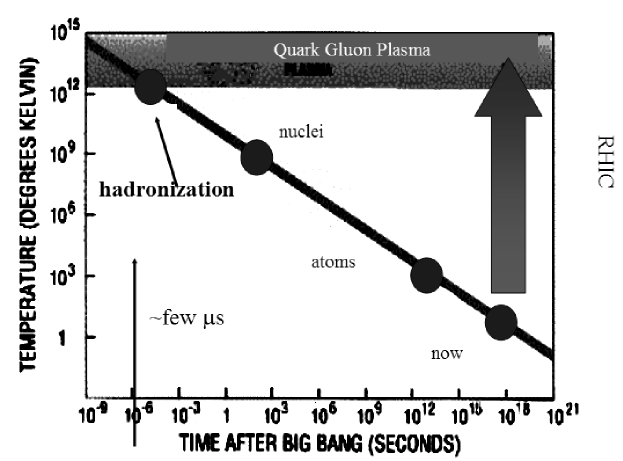
Figure 1.1: Big Bang timeline and Quark-Gluon-Plasma (QGP).

1.1 Ultrarelatvistic Heavy Ion Collisions and QGP

It has been theorised that if heavy nuclei are smashed together at very high energies (Ultrarelativistic heavy ion collisions) by means of particle accelerators, we might be to recreate the conditions that existed in the universe in that early epoch, in the lab. At sufficiently high energies, it is expected that the kinetic energy of the colliding nuclei gets converted into heat, leading to a phase transition into a new state of matter: the Quark-Gluon Plasma (QGP), in which quarks and gluons are deconfined. Quantum Chromodynamics (QCD), the theory of the Strong Interaction predicts [2] that at a well determined temperature ($T_{c}\simeq 150-180$ MeV for zero net baryon density) ordinary hadronic matter undergoes a phase transition from color singlet hadrons to a deconfined medium consisting of colored quarks and gluons. Lattice QCD calculations predict that the energy density at this transition point: $\epsilon(T_{c})\simeq 0.7-1.0$ GeV/fm³, almost 10 times the density of nuclear matter. A phase diagram of nuclear matter in equilibrium is shown in Figure 1.2.

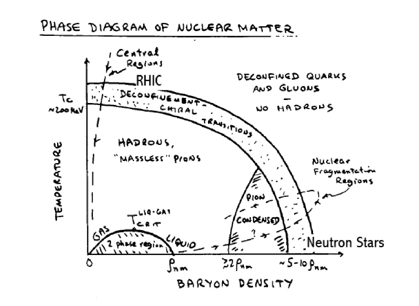
Figure 1.2: A phase diagram of nuclear matter (nuclear density along $x$-axis and temperature along $y$-axis) shows how deconfinement can occur extreme conditions of temperature (Big Bang, RHIC) and density (dense stellar matter like neutron stars). This figure is taken from 1983 NSAC Long Range Plan [3].

The holy grail of ultrarelativistic heavy ion collisions is the discovery and characterisation of the Quark-Gluon Plasma (QGP). Discovering the QGP is not an easy task, because we never see the bare quarks and gluons. Even if QGP is produced in an experiment, it subsequently hadronizes into the usual menagerie of hadrons. So we never get to directly see the QGP, and can only hope to infer it’s existence from indirect means. Some of the traditional QGP signatures are briefly outlined below:

1. Dilepton production: A quark and an anti-quark can interact via a virtual photon $\gamma^{*}$ to produce a lepton and an anti-lepton $l^{+}l^{-}$ (often called dilepton). Since the leptons interact only via electromagnetic means, they usually reach the detectors with no interactions, after production. As a result dilepton momentum distribution contains information about the thermodynamical state of the medium (For reviews see [4]).

2. Thermal Radiation: Similar to dilepton production, a photon and a gluon can be produced via $q+\bar{q}\rightarrow\gamma+g$. Since the electromagnetic interaction isn’t very strong, the produced photon usually passes to the detectors without any interactions after production. And just like dileptons, the momentum distribution of photons can yield valuable information about the momentum distributions of the quarks and gluons that make up the plasma, giving us a window into it’s thermodynamical properties (for a review see [5]).

3. Strangeness Enhancement: Production of strange quarks requires a larger amount of energy compared to ordinary u and d quarks. The high energy densities in QGP are conducive for $s\bar{s}$ production, leading to an enhancement in the number of strange particles as compared to the strangeness production in p+p collisions [6].

4. $J/\psi$ suppression: In a Quark-Gluon-Plasma (QGP), color screening due the presence of free quarks and gluons (similar to Debye screening seen in QED), the $J/\psi$ particle — a bound state of charm and anti-charm quarks $c\bar{c}$ — can dissociate. This leads to a suppression of $J/\psi$ production, a classic signature first predicted by Matsui and Satz [7].

5. HBT: The Hanbury-Brown-Twiss effect — first used to measure the diameter of a star [8] — is also used to in high energy nuclear experiments, by measuring the space-time(or energy-momentum) correlation of identical particles emitted from an extended source. In ultrarelativistic heavy ion collisions, an HBT measurement can yield information about size and the matter distribution of the source.

6. Jet suppression: In nucleon collisions, energetic partons (jets) can be produced via hard scatterings. In presence of deconfined matter, they interact strongly, leading to energy loss $\simeq$ GeV/fm, mostly due to gluon bremmstrahlung processes. This results in a decrease in the yield of high energy particles or jet suppression [9].

Discovery of QGP is beyond the scope of this dissertation, instead we shall have to satisfy ourselves by studying the behavior of nuclear matter at extreme conditions of temperature and density, via ultrarelativistic heavy ion collisions and trying to shed some light on a) properties of the final state of produced matter, and b) the initial conditions that led to this. As a result this dissertation will have two main thrusts:

1. Exploration of the final state effects of the produced matter from Au+Au collisions at $\sqrt{s_{NN}}=200$ GeV, by studying the production of the simplest nuclei: deuterons and anti-deuterons.

2. Study the effect of cold nuclear matter in d+Au collisions at $\sqrt{s_{NN}}=200$ GeV, by looking at particle production in forward and backward directions.

1.2 Deuterons and anti-deuterons as probes of final state effects

Previous measurements indicate that high particle multiplicities [10, 11] and large $\bar{p}/p$ ratios prevail at RHIC, which is expected for a nearly net baryon free region [12, 13, 14]. As the hot, dense system of particles cools, it expands and the mean free path increases until the particles cease interacting (“freezeout”). At this point, light nuclei like deuterons and antideuterons ($d$ and $\bar{d}$) can be formed, with a probability proportional to the product of the phase space densities of it’s constituent nucleons [15, 16]. Thus, invariant yield of deuterons, compared to the protons [17, 18] from which they coalesce, provides information about the size of the emitting system and its space-time evolution. We use the PHENIX Time-Of-Flight (TOF) detector along with the central arm tracking chambers: Drift Chamber (DC) and Pad Chambers (PC3) to detect deuterons. We measure momentum and time of flight and use it to obtain the mass, which is used for particle identification (PID). Corrections are then applied to account for limited acceptance, detector efficiencies and myraid other minutae that are the bane of experimentalists all over the world. We eventually obtain the corrected invariant yields $Ed^{3}N/dp^{3}$ and look really really hard at them, paying special attention to the shapes of the spectra and compare them with proton yields to glean some information about the spacetime evolution of the collision zone.

1.3 Particle multiplicities at forward and backward rapidities as probes of initial state effects

Particle multiplicities have yielded some of the most interesting insights at RHIC (Relativistic Heavy Ion Collider). Data from the Au + Au collisions at $\sqrt{s_{NN}}=200$ GeV at mid-rapidity indicated a suppression [19, 20, 21, 22] of particle yields as compared to the expectation from naive scaling of p+p collisions. This was consistent either with a) jet suppression i.e, suppression of high $p_{T}$ particles due to energy loss in the deconfined medium or b) due to the depletion of low-$x$ partons due to gluon saturation processes as predicted by the Color-Glass Condensate (CGC) hypothesis. In order to figure out whether this suppression in Au+Au collisions was due to final state effects (the Quark-Gluon-Plasma (QGP)) or due to initial state effects (gluon saturation effects), a control experiment was done by colliding deuteron and gold nuclei at the same energy. The Run 3 data with d + Au collisions at $\sqrt{s_{NN}}=200$ GeV, showed an enhancement at mid-rapidity [23, 24]. Similar effects have been seen at lower energies and go by the name of Cronin effect and are usually attributed to multiple scattering of partons in the initial state. Obviously this was inconsistent with the CGC (gluon saturation) hypothesis, which predicted a suppression in particle multiplicities [25, 26, 27] for d+Au collisions. However, all hope wasn’t lost: the scale at which the gluon saturation effects occur, provided an escape hatch and it turns out that although particle multiplicities are not suppressed at mid-rapidity, if we look at forward rapidity (in the deuteron going direction) we can explore the low-$x$ region of the Au nucleus. And depending upon the saturation scale, we might be able to see suppression. In the second half of this dissertation, we seek to measure charged hadron multiplicities at forward rapidity (approximate pseudorapidity range $1.2<\eta<2.0$) using the PHENIX Muon Arms (which b.t.w weren’t supposed to detect hadrons). By looking at the particle multiplicities scaled with those at peripheral collisions, which is the lazy man’s way of getting around the need to use p+p data, at forward and backward rapidities and their variation with centrality (or impact parameter) we hope to shed some light on the issue of initial conditions.

1.4 Some jargon

The field of the relativistic heavy ion physics is saturated with jargon, a minefield for the uninitiated. Before we embark on the rest of this dissertation, here is a brief description of some of the commonly used terms:

• Center of mass energy: a.k.a. $\sqrt{s}$, this is the Lorentz invariant quantity:

  $$s=(p_{1}+p_{2})_{\mu}(p_{1}+p_{2})^{\mu}$$ (1.1)

  For nuclei with energy $E_{i}$ and 3-momentum $\mathbf{p_{i}}$, it reduces to:

  $$\sqrt{s}=\sqrt{m_{1}^{2}+2E_{1}E_{2}-2\mathbf{p_{1}\cdot p_{2}}+\mathbf{m_{2}^{2}}}$$ (1.2)

  For instance at RHIC (Run 2 and 3), the center-of-mass energy per nucleon is $\sqrt{s_{NN}}=200$ GeV.

  

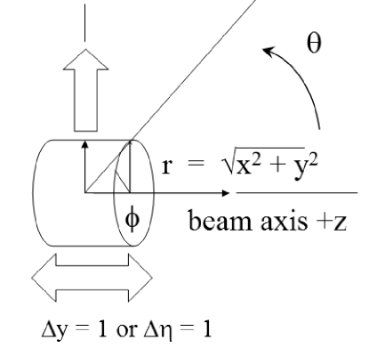
  Figure 1.3: Beam axis, transverse momentum $p_{T}$ and rapidity $y$.

• Tranverse momentum $p_{T}$: this is simply the projection of a particle’s momentum perpendicular to the collision axis: $z$ (see Figure 1.3).

  $$p_{T}=p\sin\theta$$ (1.3)

  where $\theta$ is the polar angle along the $z$-axis. A common variable derived from this is the transverse energy (or mass) $m_{T}=\sqrt{p_{T}^{2}+m_{0}^{2}}$.

• Rapidity $y$: this defines the longitudinal motion scale for a particle of mass $m_{0}$ moving along $z$-axis (see Figure 1.3):

  $$y=\frac{1}{2}\log\left(\frac{E+p_{z}}{E-p_{z}}\right)$$ (1.4)

  Since there is cylindrical symmetry around the collision axis, this allows us to describe the 4-momentum of particle in terms of its transverse momentum $p_{T}$, rapidity $y$ and the transverse energy $m_{T}$ as:

  $$p^{\mu}=(m_{T}\cosh y,p_{T}\cos\phi_{0},m_{T}\sinh y)$$ (1.5)

• Pseudorapidity $\eta$: derived from rapidity (Eq. 1.4), this variable is used when the particle in question is unidentified i.e., $m_{0}$ is not known:

  $$\eta=-\log\left(\tan\frac{\theta}{2}\right)$$ (1.6)

  Where $\theta$ is the angle w.r.t. the beam axis. $\eta$ is often used to describe geometrical acceptances of detectors.

• Invariant yield: the invariant differential cross section of a particle is the probability of obtaining $d^{3}N$ particles in the phase space volume $dp^{3}/E$ in a given number of events $N_{event}$:

  $$\frac{1}{N_{event}}E\frac{d^{3}N}{dp^{3}}=\frac{d^{3}N}{N_{event}p_{T}dp_{T}dy}$$ (1.7)

  In cylindrical coordinates $dp^{3}=dp_{x}dp_{y}dp_{z}$ reduces to $p_{T}dp_{T}d\phi m_{t}\cosh ydy$. Due to azimuthal symmetry we get a factor of $1/2\pi$, resulting in the form:

  $$\frac{1}{N_{event}}E\frac{d^{2}N}{dp^{2}}=\frac{d^{2}N}{2\pi N_{event}p_{T}dp_{T}dy}$$ (1.8)

  Using $dN/p_{T}dp_{T}=dN/m_{T}dm_{T}$, we get our final form:

  $$\frac{1}{N_{event}}E\frac{d^{2}N}{dp^{2}}=\frac{d^{2}N}{2\pi N_{event}m_{T}dm_{T}dy}$$ (1.9)

• Centrality: when the two nuclei collide, there can be range of impact parameters. Events with a small impact parameter are known as central events whereas events with a large impact parameter are called peripheral (see Figure 1.4), and the variation in impact parameters is called centrality.

  

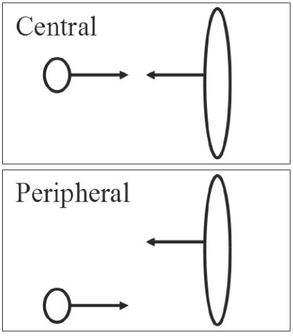
  Figure 1.4: Centrality is related to impact parameter: large impact parameter events are called peripheral and small impact parameter events are called central.

• Minimum Bias: this is the collection of events containing all possible ranges of impact parameters. This is important so that our data does not have any bias due to events that might be triggered by specific signals e.g. presence of a high $p_{T}$ particle.

1.5 Organization of thesis

This work is organised as follows: in Chapter 2 we describe the experimental setup at PHENIX. Our measurements of deuterons and anti-deuterons are described in Chapters 3 and 4. Chapters 5 discusses the background for the nuclear modification factor, while Chapters 6 and 7 are devoted to the measurement of particle multiplicities at forward (and backward) rapidities. Finally Chapter 8 summarizes all our results. Bon Voyage!

Chapter 2 Experimental Facilities and Setup

In this chapter we shall give an overview of the Relativistic Heavy Ion Collider (RHIC) and the PHENIX detector [28] alongwith the subsystems that were used for deuteron/anti-deuteron measurement.

2.1 RHIC facility

In order to have any hope of discovering the Quark-Gluon-Plasma, experimentalists have tried to collide heavy nuclei at the highest possible energies obtainable subject to the usual constraints of technology and funding. Most of the past experiments have been fixed target experiments, in which a beam of a given species, e.g. proton (p) or lead (Pb) at CERN Super Proton Synchrotron (SPS), is incident on a fixed target of the appropriate material e.g. Pb at SPS. Since the lab frame is not same as the beam frame, for a given beam energy, the actual center-of-mass energy is lesser as compared to a colliding beam accelerator like RHIC. Typical center-of-mass energies at the Alternating Gradient Synchrotron (AGS) at BNL were in the range 2.5 – 4.5 GeV, and at SPS typical $\sqrt{s}$ = 17 GeV (for Pb+Pb).

RHIC consists of 2 counter-circulating rings capable of accelerating any nucleus on any other, with a top energy (each beam) of 100 GeV/nucleon Au+Au and 250 GeV polarized p+p. The tunnel is 3.8 km in circumference and contains powerful superconducting dipole magnets to guide the beams at these energies.

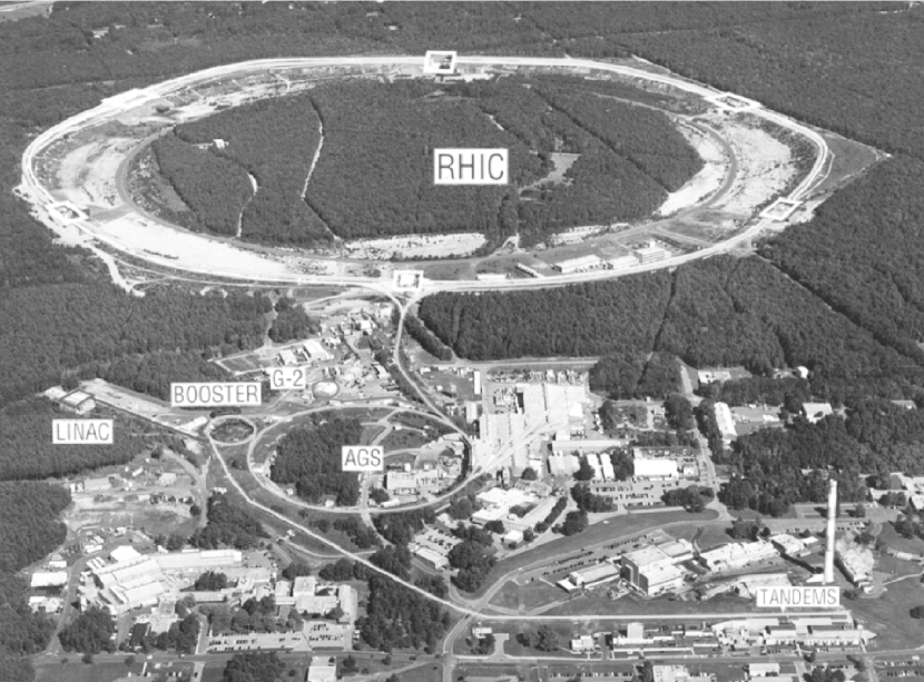
Figure 2.1: A picture of the Relativistic Heavy Ion Collider (RHIC) complex at Brookhaven National Lab (BNL) in Long Island, NY. The RHIC ring with associated systems: Tandems and AGS booster can also be seen.

Before the high energy heavy ion collisions can occur, the ions undergo several steps:

1. After removing some of the electrons from the atom, the Tandem Van de Graaff uses static electricity to accelerate the resulting ions into the the Tandem-to-Booster line (TTB). For p+p collisions, the Linear Accelerator (Linac) is used to provide energetic protons ($\approx$ 200 MeV).

2. The Booster synchrotron is a compact, powerful circular accelerator that propels the ions closer to the speed of light ($\approx$ 37%) and feeds them into the Alternating Gradient Synchrotron (AGS).

3. The AGS further accelerates the ions to 99.7% of the speed of light and injects them into the AGS-To-RHIC (ATR) transfer line, where a switching magnet directs the ion bunches to either the clockwise RHIC ring or the anti-clockwise RHIC ring.

4. Once in the RHIC rings, the ions are accelerated by radio waves (RF) to $\gamma$ = 70 or equivalently 99.995% the speed of light. Finally they are collided at the six interaction points where the four experiments reside: BRAHMS, PHENIX, PHOBOS and STAR. A typical central Au+Au event as taken in the PHENIX detector is shown in Figure 2.2.

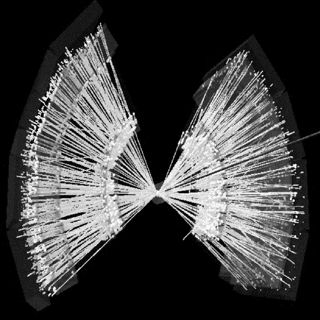
Figure 2.2: View of a central Au+Au event in PHENIX as taken in Run 2 (2002).

2.2 PHENIX detector overview

PHENIX [28] (Pioneering High Energy Nuclear Interaction eXperiment) is a versatile detector designed to study a maximal set of observables including the production of leptons, photons and hadrons over a wide momentum range. It is capable of taking events at a high rate and do selective triggering for rare processes. A detailed overview of PHENIX and its subsystems is given in Reference [28].

PHENIX consists of four spectrometers: Central Arms (East and West) at midrapidity ($|\eta|<0.35$) and the Muon Arms (North and South) at forward and backward rapidities. The detector layout in front and side view can be seen in Figure 2.3). The information from the PHENIX Beam-Beam Counters (BBC) and Zero-Degree Calorimeters (ZDC) is used for triggering and event selection. The BBCs are Čerenkov-counters surrounding the beam pipe in the pseudorapidity interval $3.0<|\eta|<3.9$, and provide the start timing signal. The ZDCs are hadronic calorimeters 18 m downstream of the interaction region and detect spectator neutrons in a narrow forward cone.

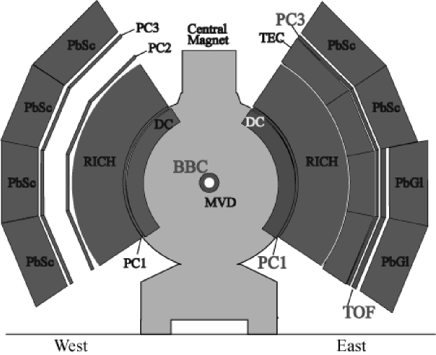
Figure 2.3: Top panel shows Front view of PHENIX (beam going into the page) showing the Central Arm with the Time-Of-Flight (TOF) detector as in Run 2 (2002). The bottom panel shows the PHENIX Muon Arms at forward and backward rapidities as set up in Run 3 (2003).

2.3 Central Arms

The Central Arm Detectors are placed radially around the beam axis extending from 2.5 m to 5 m. See top panel in Figure 2.3 for a schematic drawing the PHENIX Central Arms. They contain the following subsystems:

1. Central Magnets (CM) create an axial field around the interaction vertex with a field integral $\approx$ 0.78 T.m. perpendicular to the beam axis, with a uniformity of 2 parts in $10^{3}$. This field bends the tracks into the detector acceptance and helps the tracking detectors in momentum determination.

2. Charged tracking chambers: there are two Drift Chambers (DC), three Pad Chambers (PC) and one Time Expansion Chamber (TEC). The DC determines $p_{T}$ by measuring the charged particle trajectories in $r-\phi$ plane, as they curve in the axial magnetic field produced by the Central Magnets. The PCs aid measurement of longitudinal momentum and get 3D hits for pattern recognition by providing spatial resolution ($\simeq$ few mm) along $r-\phi$ and $z$ directions. The TEC uses differential energy loss of a traversing particle to improve $e,\pi$ seperation and can help in track reconstruction using drift times of ionization products in a gas mixture in a manner similar to DC.

3. Ring Imaging Cherenkov Detector (RICH) (one in each arm) uses photomultiplier tubes (PMTs) to detect electrons via their characteristic Cherenkov emissions. Since electrons have a low mass, they emit Cherenkov light at lower momenta as compared to other “contaminants” like pions.

4. Time-Of-Flight system (TOF) gives accurate measurement of the time of flight of a particle from vertex, aiding in particle identification (PID).

5. Electromagnetic Calorimeters measure energy deposition from e.m. showers , using two methods: Lead Glass (PbGl) and Lead Scintillator (PbSc). They are unique in being able to detect $\gamma$s (photons) and $\pi^{0}$s.

In our first analysis ($d$, $\bar{d}$ measurement) we primarily used the Drift Chamber and the Time-Of-Flight subsystems. These will be discussed in more detail in subsequent sections. The Muon Arms — used in the second analysis (hadron multiplicities in forward and backward rapidities) will be discussed in Chapter 5.

2.3.1 Drift Chambers

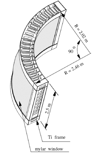
Figure 2.4: Geometry of the DC, showing the titanium frame and 20 keystones.

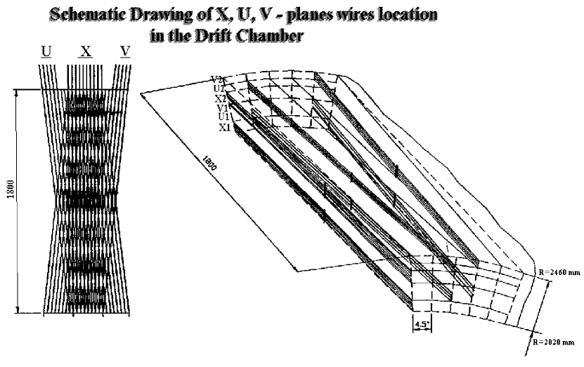
Figure 2.5: Arrangement of the X, U and V wires in the DC.

The PHENIX Drift Chambers are wire chambers and reconstruct the trajectory of a particle by using the time difference of the primary ionization (when the particle first passes through the detector) and the time the charge signal arrives on the sense wire. They are cylindrically shaped and located radially 2 to 2.4 m from the $z$-axis, and 2 m transversally along the beam direction, and each have an azimuthal acceptane of 90^o. They consist of two independent gas volumes in East and West Arms, enclosed by 5 mil Al mylar windows in a cylindrical titanium frame. Each chamber is subdivided into 20 equal sectors (called keystone) of 4.5^o in $\phi$ each of which contains 6 wire modules stacked radially: X1, U1, V1, X2, U2 and V2. Figure 2.4 shows the geometry of the DC frame. Each module has 4 sense (anode) planes and 4 cathode planes forming cells wth 2-2.5 cm drift space in $\phi$ direction. The X wires run along $z$-axis and can only reconstruct $x-y$ information, whereas the U and V layers are tilted $\approx\pm 6^{o}$ to the $z$-axis and are called stereo layers as they can be used to obtain $z$ information. A schematic diagram showing the relative arrangement of the U, V and X layers in DC is shown in Figure 2.5. In addition to the cathode and the sense (anode) wires, the DC has potential and gate wires to shape the field and remove front back ambiguity. In total the DC has 6500 anode wires and about 13, 000 readout channels. A 50/50 mixture of argon and ethane is used as the working gas in the chambers. An angular deflection $\alpha$ in the magnetic field alongwith the measured hits in the DC are used to reconstruct the momentum of the particle. The DC was designed with a single wire resolution of 150 $\mu$m and single wire efficiency greater than 99% for good tracking efficiency for high multiplicities at RHIC.

2.3.2 Time-Of-Flight

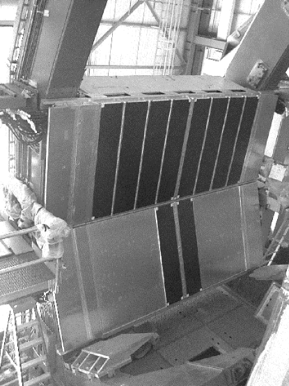
Figure 2.6: The TOF with 8 panels in the upper sector and 2 panels in the lower sector, as mounted in the East Arm.

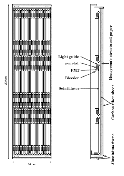
Figure 2.7: Diagram of a single TOF panel showing the plastic scintillator with PMTs at each end with corresponding light guides and supports.

The Time-Of-Flight subsystem, used as a particle identification device for hadrons, is present only in the East Arm and covers $\pi/4$ in azimuth. A picture of the TOF detector mounted in the East Arm is shown in Figure 2.6. It is located 5.0 m away from the vertex and consists of 1000 elements of plastic scintillation counters with photomultiplier tube (PMT) readouts. It consists of two sectors: top sector has 8 panels and the lower sector has 2 panels. Each panel has 960 scintillator counters along $r-\phi$ direction with 1920 PMTs readouts collectively called slats. A schematic diagram showing a TOF panel with PMTs is shown in Figure 2.7. Each slat provides time and longitudinal position information of the particles that hit the slat. The timing information, alongwith the momentum from the DC enables us to determine the mass (see Eq. 3.2), thus giving us a powerful method of particle identification. More details on this are given in the next chapter.

2.4 Centrality determination

The event centrality is measured in PHENIX using the Zero Degree Calorimeters (ZDC) and the Beam Beam Counters (BBC) in conjunction. ZDCs are small hadronic calorimeters positioned 18 m upstream and downstream of the interaction point and detect the energy deposited by the spectator neutrons during the collisions. ZDCs are so postioned so that the spectator neutrons, which do not get bent by the magnets, hit them directly allowing them to be used as event triggers in each RHIC experiment. The BBCs are positioned radially around the $z$-axis at 1.44 m from the interaction point and measure charged particle multiplicities in $3.0<\eta<3.9$. The correlation between the BBC charge sum and the ZDC energy deposit enables us to determine event centrality, because the more peripheral the collision (large impact parameter) greater is number of spectator neutrons in the ZDC, whereas the more central the collision (small impact parameter) the greater is charged particle multiplicity in the BBC and correspondingly fewer spectator neutrons make it into the ZDC. Figure 2.8 shows a scatter plot of the BBC vs ZDC response.

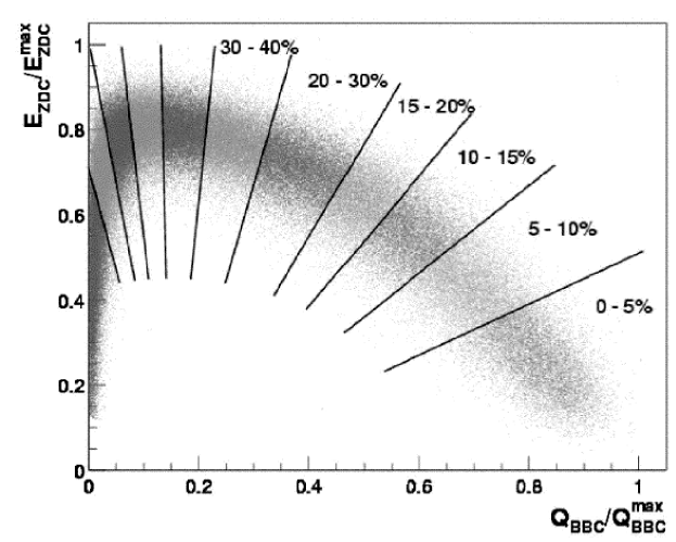
Figure 2.8: BBC vs ZDC scatter plot shows how centrality is determined in PHENIX.

2.5 Event reconstruction and data stream

At RHIC, the Au beams cross at a frequency of 9.4 MHz, which is the master clock frequency for all PHENIX subsystems. The ZDC and BBCs are used for triggering and setting the start time for an event. Whenever the vertex or the trigger subsystems are triggered (Level 1 triggers) data is sent from each of the detector subsystems by optical fiber in a raw digitized format. These Level 1 triggers allow data taking even at high collision rates by selecting interesting events e.g. an event in which a high $p_{T}$ electron was detected in the RICH. After passing the quality checks from the Online Monitoring Systems, the data is stored on tape. This raw data is now ready for calibration and reconstruction. After it is reconstructed, it saved in an easily digestible format: the nanoDSTs(nDSTs). nDSTs come in various flavors depending upon the analysis and the detector subsystem being used. For example, data from the PHENIX Central Arms is saved in Central Track Nanodsts (CNTs), which we use for the first analysis. Further details on the PHENIX data acquisition and reconstruction can be found in Reference [28].

Chapter 3 Data reduction for $d,\bar{d}$ measurement

In this Chapter, we discuss how deuterons and anti-deuterons are identified and seperated based on mass squared distributions. We obtain raw momentum distributions which are then corrected for detector acceptances, efficiency, occupancy effects. There is also a section on sources of systematical uncertainties.

3.1 Event and track selection cuts

In the Year-2 of running (2001-2002), events are selected in PHENIX using the Beam Beam Counters (BBCs), which measure the event vertex position along $z$ and also set the start time for other detectors including the Drift Chamber (DC). In conjunction with the Zero Degree Calorimeters (ZDCs), as described in the previous Chapter, BBCs are also used to determine the event centrality. For this analysis, we used Minimum Bias (MB) events, which are essentially minimally triggered events in which the BBC and the ZDC fired and are as unbiased as can be made. Event vertex was restricted to $|z|<35$ cm of the collision vertex, primarily for reasons to do with detector acceptances.

In addition we selected runs based on quality (QA), by excluding runs in which there were known subsystem problems e.g. too many dead channels in the DC, or timing problems in the Time Of Flight hodoscopes (TOFs). Bad runs were also flagged by looking at quantities like the average particle multiplicities and average momentum. In total we analysed 21.6 million minimum bias events, after excluding events rejected by our global cuts. The minimum bias cross section corresponds to $92.2^{+2.5}_{-3}$% of the total inelastic Au+Au cross section (6.8 b) [29]. In addition, tracks were selected to optimize signal and reduce background, by using the following cuts:

• DC track quality=31 or 63. These quality bit numbers give detail regarding matching the hits from the Drift Chamber UV stereo layers (in addition to the X1, X2 layers) to the Pad Chamber 1 (PC1) hits. Quality 63 is the best and indicates a unique PC1 and a unique UV hit, whereas quality 31 means an ambiguous PC1 hit and a best choice UV hit.

• $|\sigma_{\phi}(TOF,PC3)|<2.5$ and $|\sigma_{z}(TOF,PC3)|<2.5$ detector matching cuts for TOF and PC3. We look at the residual between the track projection from the vertex and actual hit, both along azimuthal $\phi$ direction and the $z$ direction. After normalizing these to account for change with momentum, we have a set of residuals in $\sigma$.

• Momentum $p>0.5$ GeV. Low momentum particles aren’t well reconstructed due to acceptance of charged particles as they bend too much, as well as energy loss effects.

• TOF $E_{loss}>0.0014\beta^{-5/3}$ GeV. The energy deposited in the TOF scintillator: $E_{TOF}$ is plotted in a scatter plot vs $\beta$ in Fig. 3.1. Using a form motivated by the Bethe-Bloch formula [30], we can exclude tracks that did not deposit the minimum ionizing particle energy, thus allowing us to reject background.

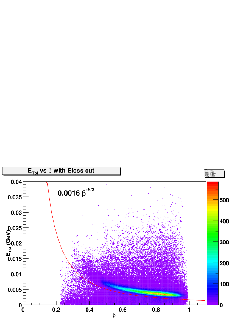
Figure 3.1: $\beta$ dependent energy loss cut for TOF to reduce background.

In addition to above cuts we excluded the low gain sector E0 of TOF (this can lead to a $z$ dependence of the mass widths) by requiring TOF Slat $<767$.

3.2 Detector resolutions

Particle identification was done by measuring the momentum $p$ using the Drift Chamber and the time-of-flight $t$ using the TOF counter. Using the standard relativistic relationship between mass and momentum:

$$p=m\frac{\beta}{\sqrt{1-\beta^{2}}}$$ (3.1)

we can obtain an expression for $m^{2}$ using momentum $p$ (from DC), the time-of-flight $t$ (from TOF), the pathlength $d$ traversed by the particle from the collision vertex to the TOF detector:

$$m^{2}=p^{2}(\frac{t^{2}c^{2}}{d^{2}}-1)$$ (3.2)

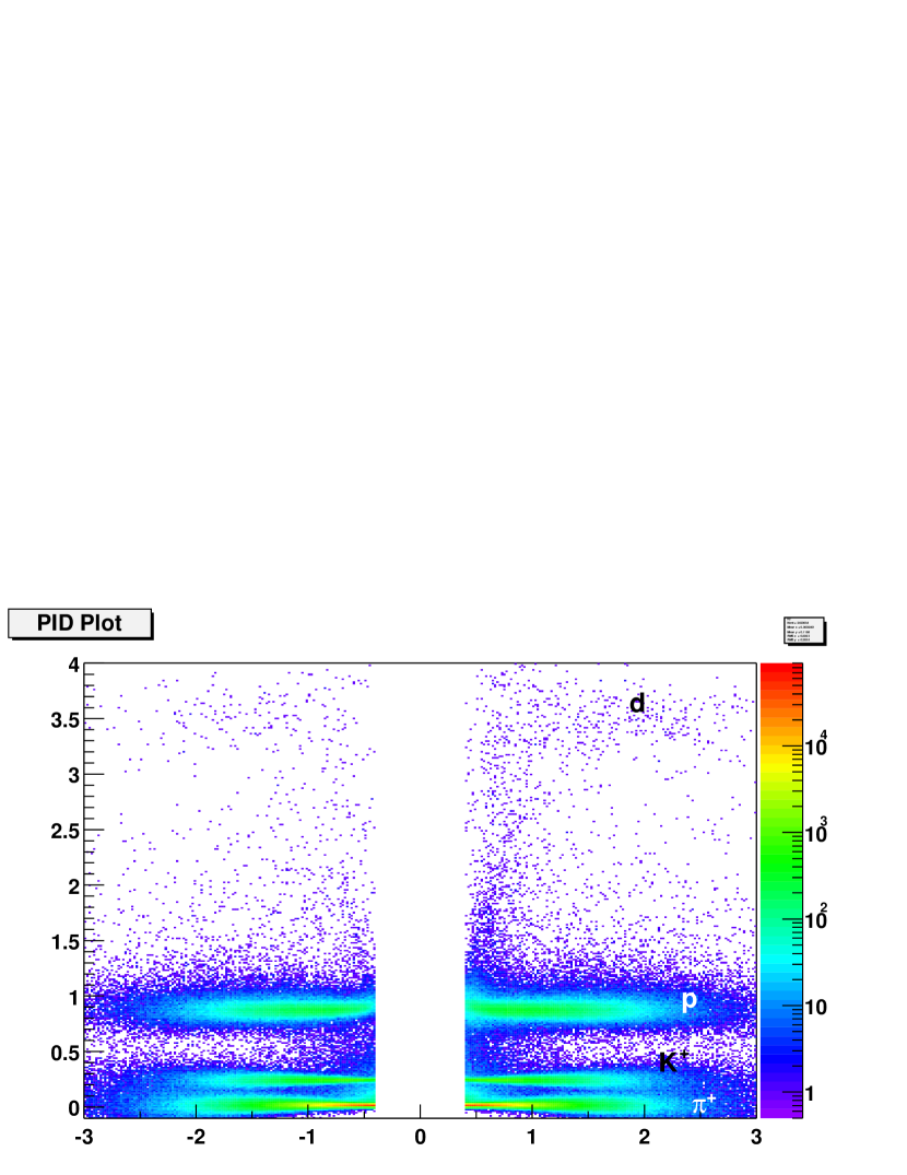
Figure 3.2: PID scatter plot with signed momentum (negatives on left and positives on right) along $x$-axis and $m^{2}$ (calculated using Eq. 3.2) along $y$-axis.

A typical PID scatter plot with $p$ along $x$-axis and $m^{2}$ along the $y$-axis is shown in Fig. 3.2. Particles are on right side (along positive $p$) and anti-particles are on the left. We can clearly see bands of different particle species like pions, kaons and protons. A faint deuteron band can also be seen.

Our ability to discriminate between different particle species depends on the resolutions of detectors being used. For example, better DC resolution enables us to go to higher values of tranverse momentum $p_{T}$ by better signal to noise ratio. Similarly improved TOF resolution will give a better seperation between particle species. One way to estimate the detector resolutions for DC and TOF is by measuring the width of the $m^{2}$ bands of particles. Since the DC determines momentum by measuring the angle by which a track bends in the magnetic field, it’s momentum resolution depends upon it’s intrinsic angular resolution $\sigma_{\alpha}$. In addition other factors like the multiple scattering of a charged particle as it travels up to the drift chamber due to the intervening matter (MVD cladding, air, DC mylar window, He-bag mylar window etc.) also play a role at different ranges. The momentum (in GeV) determined by DC is related to the angle of bending $\alpha$ (in mrad) by:

$$p=\frac{87}{\alpha}$$ (3.3)

Where, 87 mrad GeV is simply the field integral:

$$K_{1}=\int_{0.3/R_{DC}}lBdl$$ (3.4)

This gives us the momentum resolution as:

$$\left(\frac{\delta p}{p}\right)^{2}=\left(\frac{\sigma_{\alpha}}{K_{1}}p\right)^{2}+\left(\frac{\sigma_{ms}}{K_{1}\beta}\right)^{2}$$ (3.5)

where $\sigma_{\alpha}$ is the angular resolution of the DC, $\sigma_{ms}$ is the multiple scattering term and $\sigma{tof}$ is the timing resolution of the TOF. Using above equation (Eq. 3.5 we can derive a relation between the width of the $m^{2}$ bands and the DC angular resolution ($\sigma_{\alpha}$), multiple scattering ($\sigma_{ms}$) and TOF resolution ($\sigma_{tof}$):

$$\sigma_{m^{2}}^{2}=\frac{\sigma_{\alpha}^{2}}{K_{1}^{2}}\left(4m^{4}p^{2}\right)+\frac{\sigma_{ms}^{2}}{K_{1}^{2}}\left[4m^{4}\left(1+\frac{m^{2}}{p^{2}}\right)\right]+\frac{\sigma_{tof}^{2}c^{2}}{L^{2}}\left[4p^{2}\left(m^{2}+p^{2}\right)\right]$$ (3.6)

Hence by looking at the width of the $m^{2}$ distributions of various particle species we can estimate various resolution terms. In order to determine the contributions due to multiple scattering and angular resolution, we calculated the $m^{2}$ using CNTs from certain selected runs 29531, 29999, 30015 and 30069 from Run 2 Au+Au (about 2.5 million events). After making some standard cuts as before we used the measured $p$ and $t$ to make histograms of the mass squared distribution. A $m^{2}$ histogram in a given momentum range is shown in Fig. 3.3. We can see sharp pion and kaon peaks around the expected Particle Data Group [31] values, followed by a broader proton peak. And finally there is a little deuteron peak on the extreme right. As a first order estimate for particle identification, we made simple straight line cuts by assuming that all particles in the $m^{2}$ range [-0.15, 0.15] are pions, all particles in [0.15, 0.35] range are kaons and all particles in the [0.5, 1.25] range are protons. We fitted gaussians and double gaussians to the resulting $m^{2}$ histograms to each particle species. Some of these fits, for the momentum range $1.0<p<1.2$ GeV are shown for positive particles in Fig. 3.4 for pions, in Fig. 3.5 for kaons and Fig. 3.6 for protons. Systematic uncertainties in fits were obtained from the difference between the gaussian and the digaussian fits. Thus, we obtained the mean and the sigma of the $m^{2}$ bands for different momentum bins.

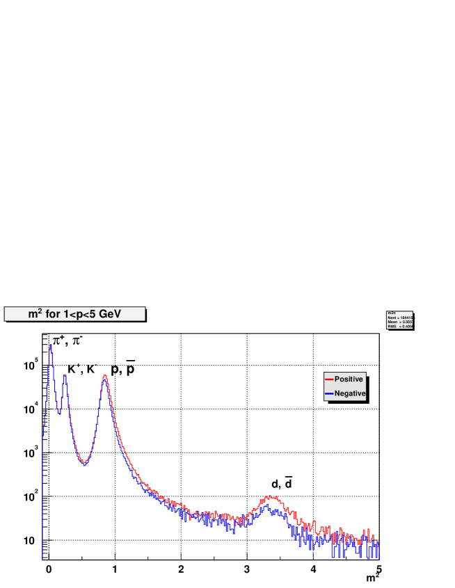
Figure 3.3: $m^{2}$ histogram showing peaks for different (anti)particle species.

Figure 3.4: Digaussian fits to $m^{2}$ histograms for pions in the momentum range $1.0<p<1.2$ GeV

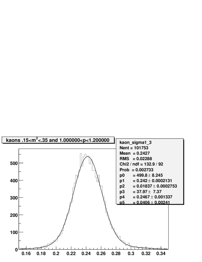
Figure 3.5: Digaussian fits to $m^{2}$ histograms for kaons in the momentum range $1.0<p<1.2$ GeV

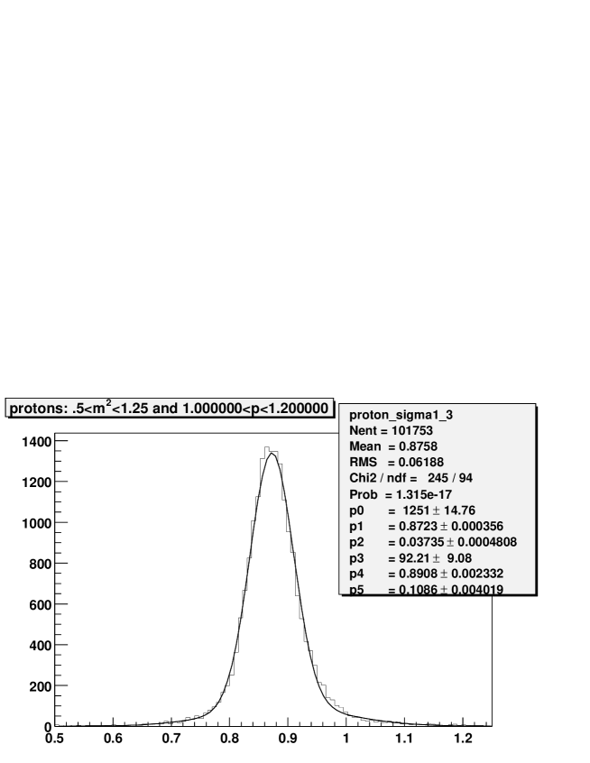
Figure 3.6: Digaussian fits to $m^{2}$ histograms for protons in the momentum range $1.0<p<1.2$ GeV

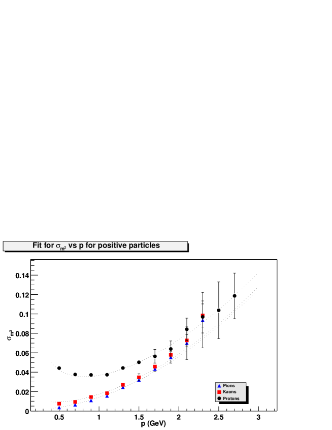
Figure 3.7: Fit for parameters for positive particles (see Table 3.1).

We made a simultaneous three parameter fit to pions, kaons and protons with $\sigma_{\alpha}$, $\sigma_{ms}$ and $\sigma_{tof}$ as the parameters, first for positive particles and then for negative particles. The fit for $m^{2}$ bands is shown in Fig 3.7 (for positive particles). From these fits we obtained $\sigma_{\alpha}$ = 0.83 mrad, $\sigma_{ms}$ = 0.92 mrad/GeV, and $\sigma_{tof}$ = 120 ps. Values of the fit parameters for Au+Au data (Run 2) are tabulated in Table 3.1.

Table 3.1: Momentum resolution parameters for Au+Au data (Run 2).

Type	$\sigma_{\alpha}$ (mrad)	$\sigma_{ms}$ (mrad GeV)	$\sigma_{tof}$ (ps)
Positives	$0.83\pm 0.09$	$0.92\pm 0.03$	$120\pm 2$
Negatives	$0.89\pm 0.07$	$0.75\pm 0.02$	$119\pm 2$

The contribution to the $m^{2}$ width of protons from each of these terms is shown in Fig. 3.8. Multiple scattering $\sigma_{ms}$ is important at low momenta and for more massive particles like protons and deuterons as it varies primarily as a function of speed $\beta$. This term alongwith acceptance effects is the main reason why our deuteron and anti-deuteron spectra are limited at the lower end of momentum around 1.1 GeV/c. At high values of momenta, our $m^{2}$ width is limited by the timing resolution $\sigma_{tof}$. Obviously the better our resolution, narrower are the $m^{2}$ bands and better is our particle identification (PID).

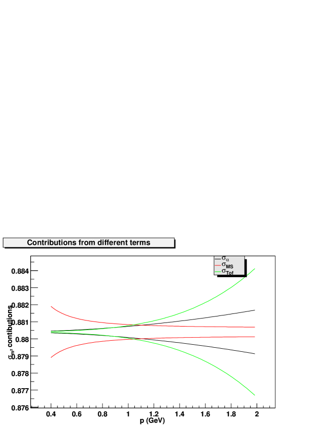
Figure 3.8: Contribution to the PID cuts for protons from different terms

We also put in new calibrations for drift velocity $v_{d}$, by looking at the variation of proton mass width as a function of change in drift velocity $\Delta v_{d}$, (see Fig. 3.9) and taking the value of $v_{d}$ which leads to the narrowest mass width for protons. If we assume an angular resolution of 0.83 mrad, then at low momenta momentum resolution is limited by multiple scattering to $\delta p/p\approx 0.7$% and at high momenta it is limited by the angular resolution of the DC to $\delta p/p^{2}\approx 1.0\pm 0.1$ %. This is often represented as: $\delta p/p\approx 0.7\%\oplus 1\%p$ GeV/$c$. A plot of the momentum resolution as a function of $p_{T}$ is shown in Fig 3.10. We also checked that the momentum resolution does not vary as a function of centrality.

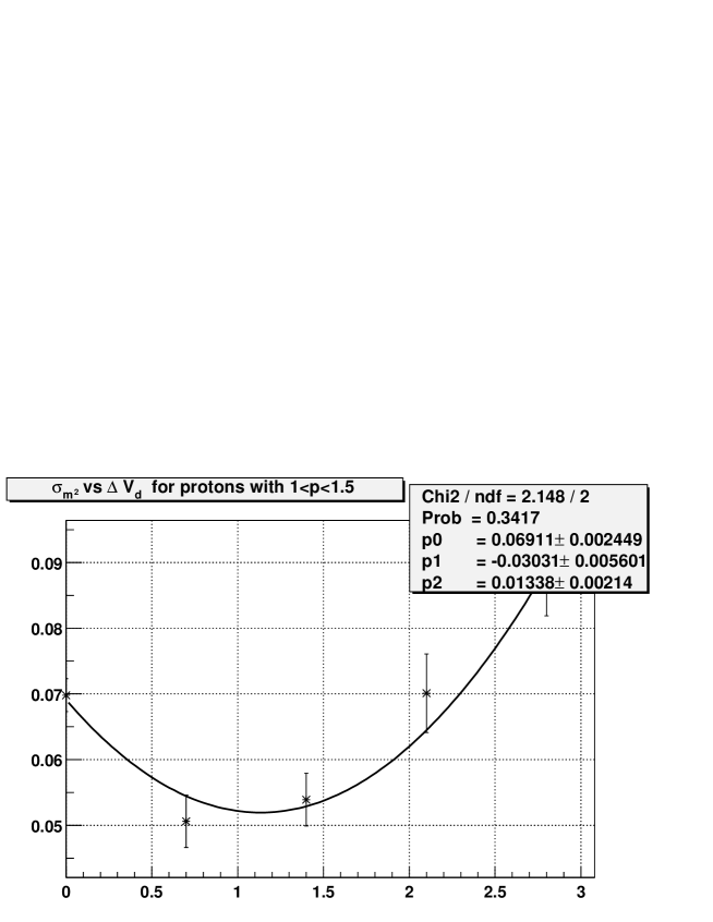
Figure 3.9: Width of proton $m^{2}$ vs change in drift velocity $v_{d}$.

A comparision of the $m^{2}$ values of particles with those from the Particle Data Book [31] indicated a 4% discrepancy. And these values changed with momentum. This is commonly seen if there is an offset in the momentum scale as well as offset in TOF timing. A correction of about 2% $\pm$ 0.7% for the momentum scale was applied to remove these offsets.

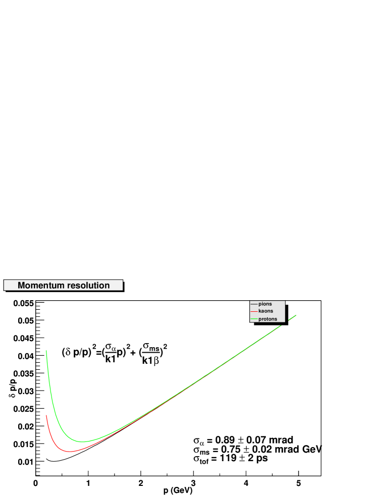
Figure 3.10: Momentum resolution

3.3 Signal Extraction

Finally after all these cross checks on resolutions we are now ready to start extract (anti)deuteron signal from our $m^{2}$ histograms. As mentioned before, in Fig. 3.3, we can see sharp pion and kaon peaks around followed by a broader proton peak. And finally there is a little deuteron peak on the extreme right. Our simplistic PID technique of using just straight line cuts by taking all particles in a given $m^{2}$ range as a particular particle species (e.g., pions in $m^{2}$ range of [-0.15, 0.15]) is not good enough. As we can see there is background under the $d$, $\bar{d}$ peak from various sources like mismatched momenta and tail from proton peaks. A simple straight line cut will include too much background, so we fit a gaussian with a background function (either $e^{-x}$ or $1/x$) and extract the number of deuterons under the gaussian.

We made several $m^{2}$ histograms around the expected mass squared value of deuterons in different momentum bins of 400 MeV/c widths (except last bin, which is 800 MeV/c wide to increase statistics) from 1.1 to 4.3 GeV/c. For the minimum bias data, the fits for deuterons are shown in Fig. 3.13 and for anti-deuterons in Fig. 3.16. This was repeated for two other centrality classes — 0-20% and 20-92% — in Figs.  3.11,  3.12,  3.14 and  3.15.

Using the gaussian fits, we can calculate the raw count of deuterons by:

$$N_{d}=\sqrt{2\pi}A_{d}\sigma_{d}$$ (3.7)

where $A_{d}$ is the amplitude and $\sigma_{d}$ is the sigma of the gaussian. We used $N_{d}$ as a fit parameter instead of amplitude, by inverting the above relation to obtain $A_{d}$ in terms of $N_{d}$. In this case the area under the gaussian is written as:

$$\frac{N_{d}}{\sqrt{2\pi}\sigma}\exp\left({-\frac{x^{2}}{2\sigma^{2}}}\right)$$ (3.8)

The width of the gaussian was restricted within a narrow range using our knowledge of the momentum resolution parameters as determined before 3.6. A plot showing the variation of mean and the sigma of the peak obtained by this method is shown in Fig. 3.17.

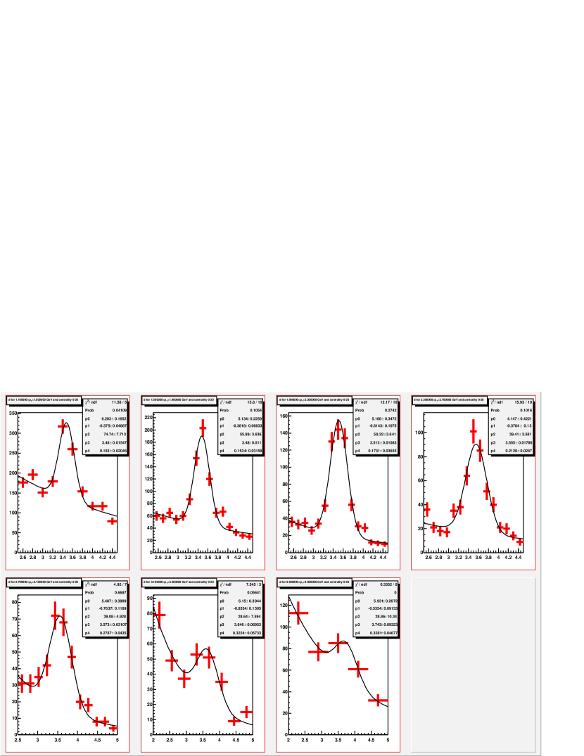
Figure 3.11: Gaussian fit with $e^{-x}$ background for d in 0-20% centrality for $p_{T}$ ranges 1.1-1.5, 1.5-1.9, 1.9-2.3, 2.3-2.7, 2.7-3.1, 3.1-3.5, 3.5-4.3 GeV/c (starting from top left).

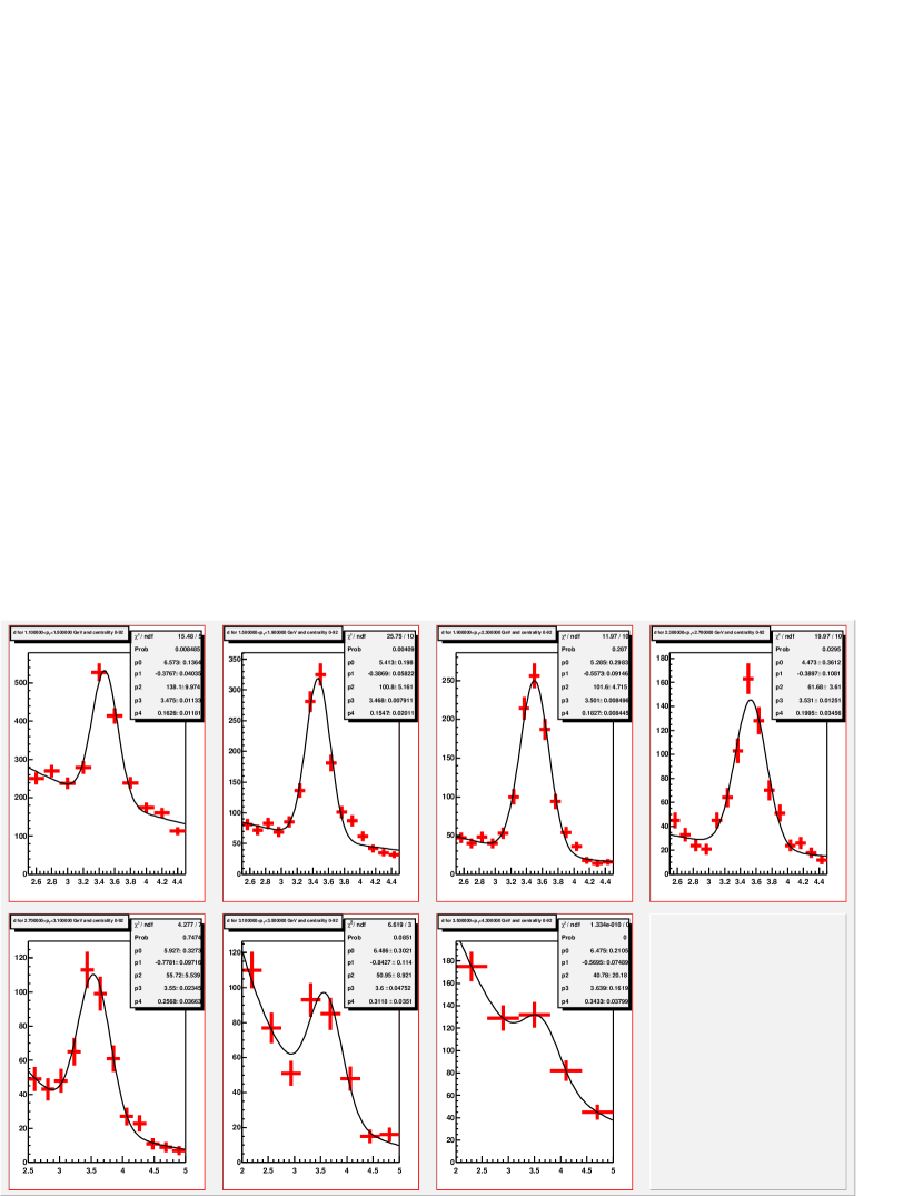
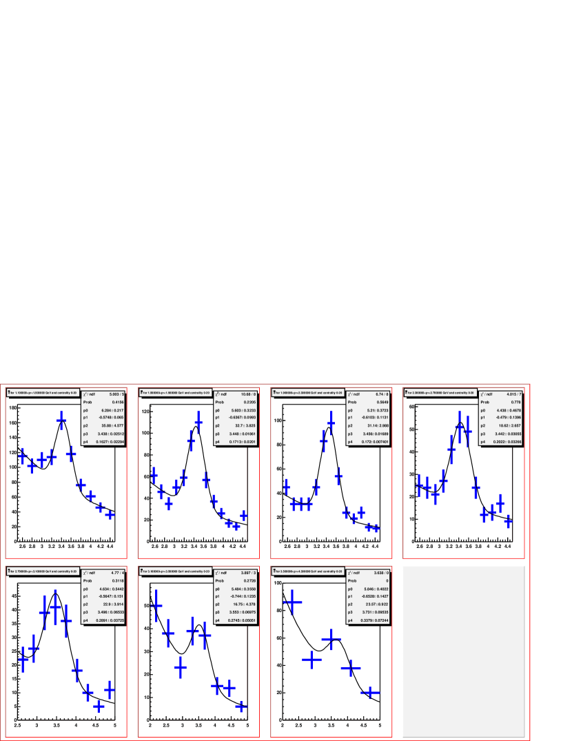
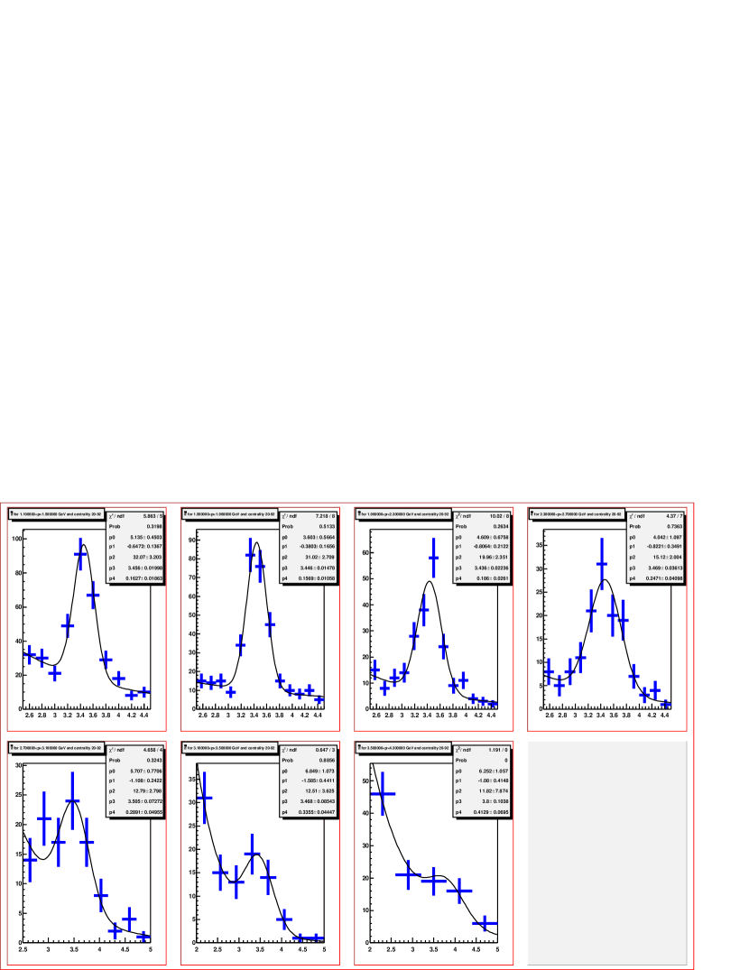
Figure 3.12: Gaussian fit with $e^{-x}$ background for d in 20-92% centrality for $p_{T}$ ranges 1.1-1.5, 1.5-1.9, 1.9-2.3, 2.3-2.7, 2.7-3.1, 3.1-3.5, 3.5-4.3 GeV/c (starting from top left).

Figure 3.13: Gaussian fit with $e^{-x}$ background for d in 0-92% centrality for $p_{T}$ ranges 1.1-1.5, 1.5-1.9, 1.9-2.3, 2.3-2.7, 2.7-3.1, 3.1-3.5, 3.5-4.3 GeV/c (starting from top left).

Figure 3.14: Gaussian fit with $e^{-x}$ background for dbar in 0-20% centrality for $p_{T}$ ranges 1.1-1.5, 1.5-1.9, 1.9-2.3, 2.3-2.7, 2.7-3.1, 3.1-3.5, 3.5-4.3 GeV/c (starting from top left).

Figure 3.15: Gaussian fit with $e^{-x}$ background for dbar in 20-92% centrality for $p_{T}$ ranges 1.1-1.5, 1.5-1.9, 1.9-2.3, 2.3-2.7, 2.7-3.1, 3.1-3.5, 3.5-4.3 GeV/c (starting from top left).

Figure 3.16: Gaussian fit with $e^{-x}$ background for dbar in 0-92% centrality for $p_{T}$ ranges 1.1-1.5, 1.5-1.9, 1.9-2.3, 2.3-2.7, 2.7-3.1, 3.1-3.5, 3.5-4.3 GeV/c (starting from top left).

The raw spectra deuteron (anti-deuteron) spectra are shown in Fig  3.18 and the raw counts (for 21.6 M events) as extracted from the fitting procedure are listed in Table 3.2. We notice that the raw spectra fall off at low $p_{T}$. This is primarily because of the heavy mass of deuterons, which leads to a smaller acceptance. A plot showing the PHENIX acceptance for different particle species as a function of momentum and rapidity is shown in Fig. 3.19.

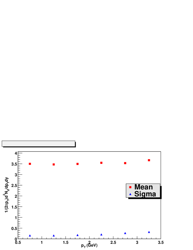
Figure 3.17: Variation of the mean and sigma of $m^{2}$ centroid for anti-deuterons

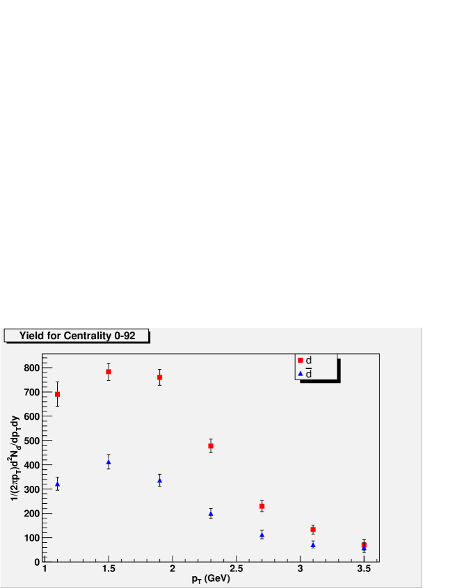
Figure 3.18: Raw spectra for deuterons and anti-deuterons (min. bias)

Table 3.2: Raw Yields vs $p_{T}$ (mid-point) for different centralities

Centrality	$p_{T}$ GeV	Raw counts for $d$	Raw counts for $\bar{d}$
	1.3	690.712 $\pm$ 49.868	322.114 $\pm$ 26.9392
	1.7	782.783 $\pm$ 35.6892	412.272 $\pm$ 29.811
	2.1	760.001 $\pm$ 32.999	336.306 $\pm$ 24.556
Min. Bias	2.5	477.309 $\pm$ 27.9426	199.812 $\pm$ 20.3159
	2.9	229.359 $\pm$ 23.4378	112.669 $\pm$ 17.5777
	3.3	133.208 $\pm$ 18.8056	71.6043 $\pm$ 14.913
	3.9	69.7416 $\pm$ 21.3508	58.9473 $\pm$ 20.2146
	1.3	378.291 $\pm$ 31.4306	171.522 $\pm$ 21.9933
	1.7	443.66 $\pm$ 28.3072	210.57 $\pm$ 20.5607
	2.1	449.276 $\pm$ 26.1366	207.874$\pm$ 20.1791
0-20%	2.5	308.455 $\pm$ 23.2434	116.245 $\pm$ 16.7561
	2.9	145.113 $\pm$ 19.6931	75.9248 $\pm$ 14.242
	3.3	72.1734 $\pm$ 14.8395	46.3732 $\pm$ 12.3767
	3.9	50.032 $\pm$ 18.0059	40.9745 $\pm$ 15.8305
	1.3	314.905 $\pm$ 24.9601	153.976 $\pm$ 15.5005
	1.7	338.779 $\pm$ 21.5489	203.035 $\pm$ 16.7537
	2.1	313.051 $\pm$ 20.1975	129.831 $\pm$ 13.8321
20-92%	2.5	177.778 $\pm$ 16.5595	76.1233 $\pm$ 11.838
	2.9	87.5999 $\pm$ 13.9707	39.7836 $\pm$ 10.2824
	3.3	70.3182 $\pm$ 13.1204	31.136 $\pm$ 8.79026
	3.9	31.368 $\pm$ 13.1671	17.3637 $\pm$ 11.5297

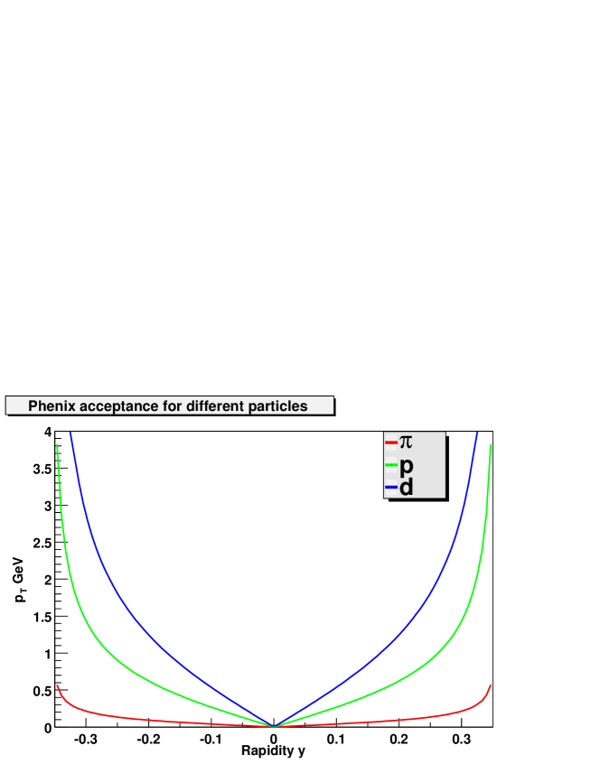
Figure 3.19: Phenix acceptance for deuterons and anti-deuterons with other particles ($\pi,K,p$).

3.4 Corrections

Before we can obtain our final spectra from the raw particle counts, we need to correct for factors like:

• Detector acceptance: limited PHENIX acceptance means our raw counts need to be corrected up.

• Detector efficiency: Detectors can be fickle, sometimes certain channels have to be switched off, at other times low voltages can lead to lower detection capabilities. This has to be corrected for.

• Track reconstruction: the algorithms that do event reconstruction and determine tracks from hits aren’t always 100% efficient. This reconstruction efficiency can also depend on event centrality. E.g. there are more tracks in central events, leading to a greater probability of error and misidentification of a track.

• Hadronic annihilation factors: the GEANT package [32], which is used to simulate how a particle tracks through a given detector does not implement hadronic interactions for clusters like deuterons. In addition, anti-deuterons also have a probability to annihilate before they are fully tracked and identified causing us to undercount them. This has be to be corrected.

• Detector occupancy effects: detector and track reconstruction efficiencies are often affected by high multiplicity events. E.g. before a slower particle like deuteron hits a detector channel, a faster particle might have hit and so the slower particle might not register. This effect is greater for heavier and slower particles like deuterons. Since this varies with particle multiplicities, it leads to a centrality dependent correction.

• Momentum bins: since particle counts are not flat over a given momentum bin putting the data points at the bin center would be incorrect. E.g. in the $p_{T}$ range 1.1 to 1.5 GeV/c the raw counts increase, as a result the midpoint of the $p_{T}$ bin is too low. This can be rectified by taking the mean $p_{T}$ of each bin using the following expression:

  $$p_{Bin}=\frac{\int_{p_{1}}^{p_{2}}p_{T}f(p_{T})dp_{T}}{\int_{p_{1}}^{p_{2}}f(p_{T})dp_{T}}$$ (3.9)

  where $f(p_{T})$ is a function (gaussian) used to fit the raw yields 3.18. Due to shape of the raw spectra, a polynomial or a gaussian give similar results.

3.4.1 Single particle efficiency

In order to correct our raw spectra due to limitations of detector acceptance, efficiencies and track reconstruction, we use Monte Carlo (MC) simulation techniques. Single particle tracks are generated and then reconstructed using PHENIX simulation package. One million deuteron (anti-deuteron) events were generated using the package EXODUS over full azimuthal coverage and rapidity $|y|<0.6$. The output files in OSCAR format were run through the PHENIX simulation package PISA. These packages try to reflect the detector characteristics as accurately as possible. The single particle tracks thus generated were reconstructed to obtain the correction factors by taking the ratio of the reconstructed $p_{T}$ distributions with the input EXODUS $p_{T}$ distributions (restricted to $|y|<0.5$ in order to get corrections for unit rapidity interval). This gives us the acceptance, efficiency of reconstruction, matching cuts and so on.

$$\frac{dN_{gen}/dp_{T}}{dN_{reco}/dp_{T}}=\epsilon_{acc}\times\epsilon_{eff}$$ (3.10)

where

$$\epsilon_{eff}=\epsilon_{track}\times\epsilon_{match}\times\epsilon_{PID}\times\epsilon_{active\ area}$$ (3.11)

In order to account for the finite momentum resolution effects the input $p_{T}$ distribution was weighted with the weight function:

$$W(p_{T})=\frac{e^{-m_{t}/T_{eff}}}{f(p_{T})}$$ (3.12)

where

$$f(p_{T})=1+10e^{-2p_{t}}$$ (3.13)

is the EXODUS low $p_{T}$ enhanced distribution. The input distribution was enhanced at low $p_{T}$ to increase our statistics since we lose low momentum particles due to acceptance effects. Since the inverse slope parameter $T_{eff}$ (used for the fit to spectra) is known to be different for different centralities, we changed it’s value to check if this has any effect on the MC for different centralities. We found no change in the correction function for different centralities.

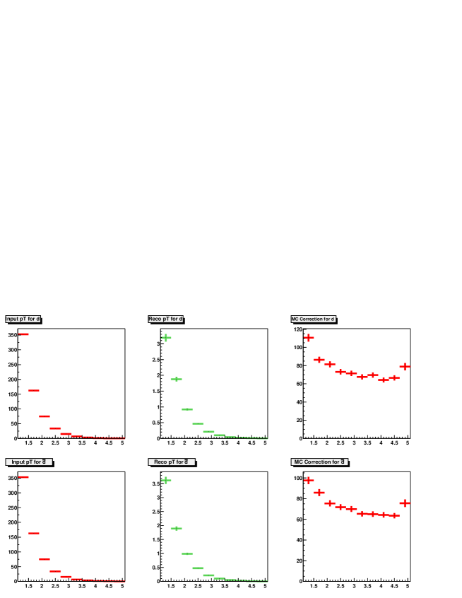
Figure 3.20: Top left panel shows input EXODUS distribution, middle panel shows the reconstructed output distribution and right panel shows the single particle MC correction as a function of $p_{T}$ for deuterons (top panels) and anti-deuterons (bottom panels) for min. bias data.

We also need to check that our MC simulations match each detector’s characteristics as accurately as possible. To cross check this, we look at track and hit distributions for each of our track cuts (like matching cuts) both in MC and data. Some comparisions for acceptances between data and MC are shown in in Appendix A. We also need to ensure that our matching cuts (or track residuals): $\sigma_{\phi}(TOF,PC3)$ and $\sigma_{z}(TOF,PC3)$ are well matched between data and MC. Matching cuts kept too wide lead to too much background, whereas if they are kept too narrow then we lose signal. If the matching cuts are not well matched between data and MC then the corrections can have errors. In order to avoid this, we plot the matching cuts $\sigma_{\phi}(TOF,PC3)$ and $\sigma_{z}(TOF,PC3)$ against variables like $z$, centrality, $p_{T}$ and so on and look for differences between data and MC. These plots are also available in Appendix A.

This finally gives us a set of bin by bin corrections for deuterons (anti-deuterons) as shown in Fig. 3.20 for minbias data. The values of the bin-by-bin corrections are tabulated in Table 3.3. This is then fit to a polynomial and used to interpolate to get corrections (see Fig. 3.21). This interpolation is necessary even though we have generated bin-by-bin corrections, because values for raw counts are being plotted at mean $p_{T}$ of each bin, instead of the midpoint of the bin.

Table 3.3: Single particle Monte Carlo corrections

$p_{T}$ GeV	Deuteron	Anti-deuteron
1.3	110.513 $\pm$ 4.2204	97.615 $\pm$ 3.50381
1.7	86.3182 $\pm$ 3.3729	85.8968 $\pm$ 3.35731
2.1	81.4226 $\pm$ 3.34997	75.51 $\pm$ 2.98608
2.5	73.1532 $\pm$ 2.98991	71.8395 $\pm$ 2.89169
2.9	71.4168 $\pm$ 2.92981	70.0016 $\pm$ 2.81757
3.3	67.5995 $\pm$ 2.78592	65.4321 $\pm$ 2.59155
3.7	69.5334 $\pm$ 2.95599	65.0881 $\pm$ 2.64015
4.1	64.1365 $\pm$ 2.69051	64.347 $\pm$ 2.613
4.5	66.524 $\pm$ 2.92311	63.553 $\pm$ 2.62167

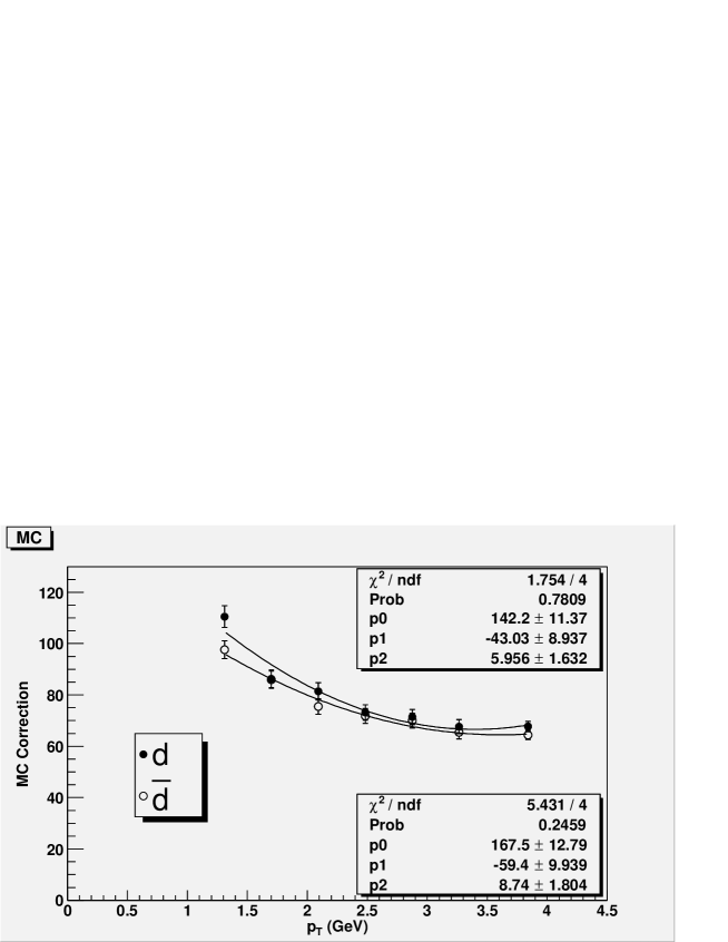
Figure 3.21: Final single particle Monte Carlo (MC) corrections with fits for interpolation

3.4.2 Loss of tracks due to occupancy effects

In high multiplicity events, tracks can be lost. Sometimes, the track reconstruction algorithms can misidentify tracks in the presence of a large number of hits. At other times the track of slower particle like a deuteron might not register at a detector, because it has already been hit by a fast particle like electron or pion. This effect is greater for heavier particles as they are slower. It also depends on the event centrality because more tracks can get misidentified in high multiplicity events. In order to correct for this, we embed a simulated single particle MC track in a real event. We then see if this simulated track gets reconstructed. We generated these corrections using code developed by Jiangyong Jia [33]. The embedding correction as a function of $p_{T}$ for different centralities is shown in Figs. 3.22,  3.23,  3.24 for the min. bias, 0-20% centrality and 20-92% centrality data respectively. The embedding correction is flat with $p_{T}$ within errors. The final values are calculated by intergrating over the entire $p_{T}$ range and are tabulated in Table 3.4.

Figure 3.22: Top left panel shows input distribution, middle panel shows the output distribution (after embedding) and right panel shows the embedding correction as a function of $p_{T}$ for deuterons (top panels) and anti-deuterons (bottom panels) for min. bias data.

Figure 3.23: Top left panel shows input distribution, middle panel shows the output distribution (after embedding) and right panel shows the embedding correction as a function of $p_{T}$ for deuterons (top panels) and anti-deuterons (bottom panels) for 0-20% centrality data.

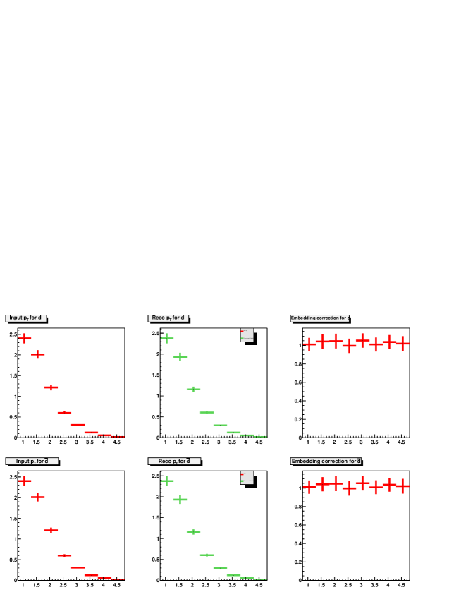
Figure 3.24: Top left panel shows input distribution, middle panel shows the output distribution (after embedding) and right panel shows the embedding correction as a function of $p_{T}$ for deuterons (top panels) and anti-deuterons (bottom panels) for 20-92% centrality data.

Table 3.4: Embedding correction

Centrality	Correction factor
Min Bias: 0-92%	1.0691 $\pm$ 0.0274
Most Central: 0-20%	1.1979 $\pm$ 0.0711
Mid-Central 20-92%	1.0224 $\pm$ 0.0310

The (anti-) proton spectra used for comparision were also corrected for feed-down from $\Lambda$ and $\bar{\Lambda}$ decays by using a simulation tuned to reproduce the particle composition: $\Lambda/p$ and $\bar{\Lambda}/\bar{p}$ measured by PHENIX at 130 GeV [34]. The systematic error in proton yields from the feed down corrections is estimated at 6 %.

3.4.3 Hadronic absorption of $d$/$\overline{d}$

Since the hadronic interactions of nuclei are not treated by GEANT, a correction needs to be applied to account for the hadronic absorption of $d$ and $\bar{d}$ (including annihilation). The $d$- and $\bar{d}$-nucleus cross sections are calculated from parameterizations of the nucleon and anti-nucleon cross sections [35]:

$$\sigma_{d/\bar{d},A}=[\sqrt{\sigma_{N/\bar{N},A}}+\Delta_{d}]^{2}$$ (3.14)

The limited data available on deuteron induced interactions [36, 37] indicate that the term $\Delta_{d}$ is independent of the nuclear mass number $A$ and that $\Delta_{d}=3.51\pm 0.25$ mb^1/2. The hadronic absorption varies only slightly over the applicable $p_{T}$ range and is $\approx$ 10% for $d$ and $\approx$ 15% for $\bar{d}$. A plot of the (anti)deuteron survival correction is shown in Fig. 3.25. Special thanks goes to Joakim Nystrand for determination of this correction. The background contribution from deuterons knocked out due to the interaction of the beam with the beam pipe is estimated using simulation and found to be negligible in the momentum range of our measurement.

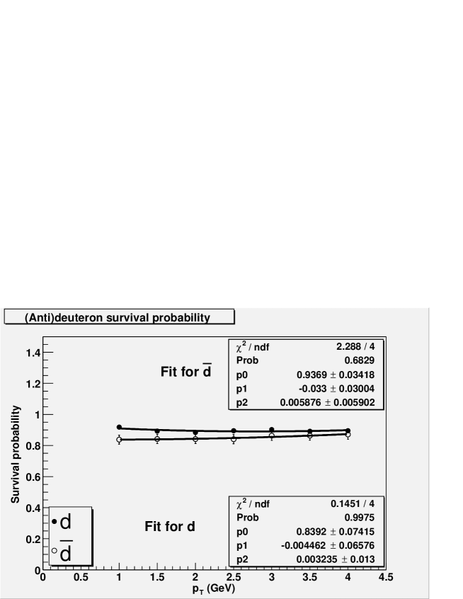
Figure 3.25: Correction for (anti-)deuteron survival vs $p_{T}$ [38].

The total error is dominated by the systematic errors in the correction factors, and we estimate these to be 1.5% (3.5%) for deuterons (anti-deuterons).

Chapter 4 $d,\bar{d}$ yields and implications

The hadrons produced in the collision zone carry information about the nature of the collision, as well its size and composition. In particular, the $p_{T}$ behaviour of the spectra can yield information about the dynamics of the collision, while the particle yields and abundances can help us to determine the chemical composition.

4.1 Spectra

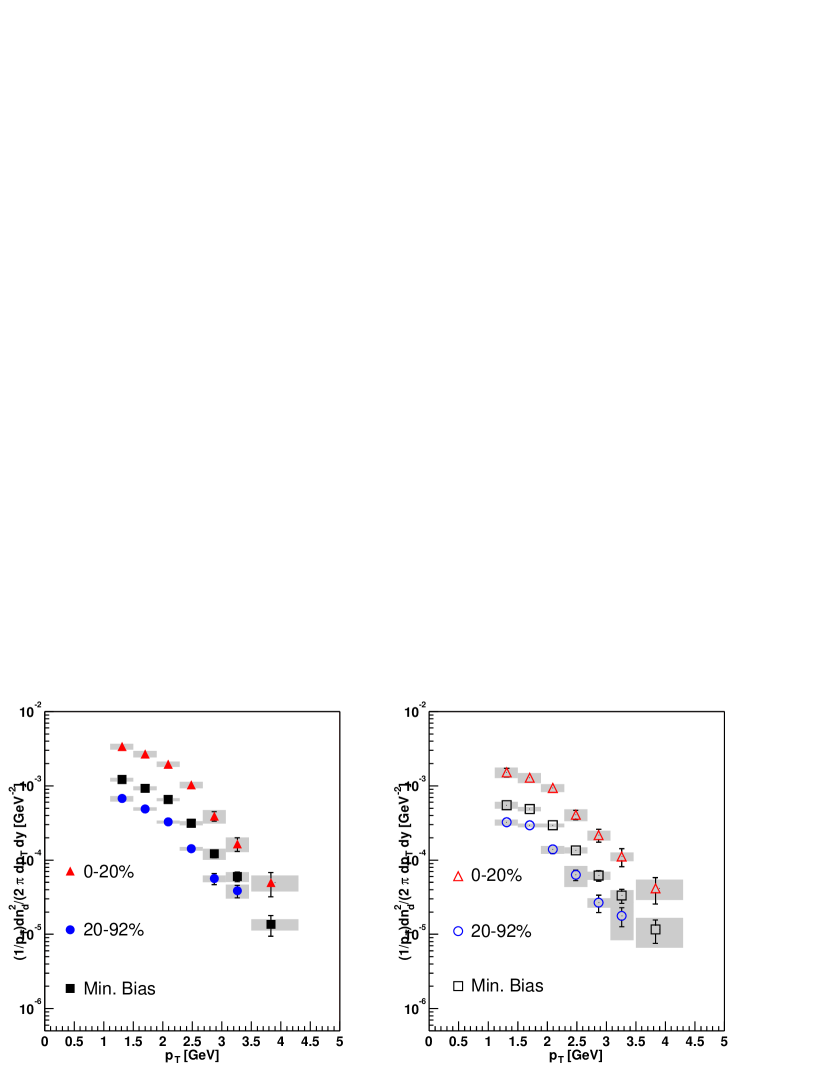
Figure 4.1: Corrected $\bar{d},d$ yields vs $p_{T}$ for different centralities.

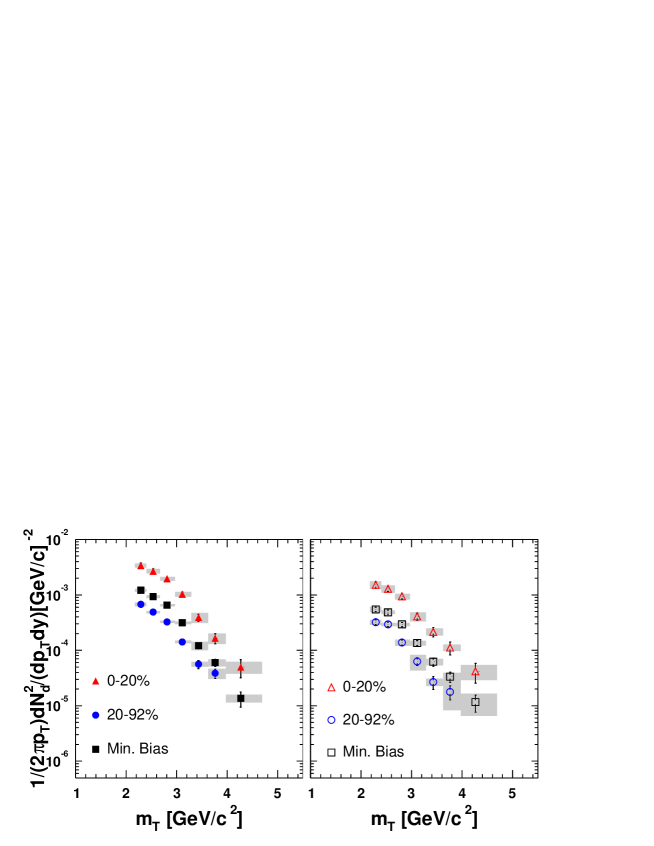
Figure 4.2: Corrected $\bar{d},d$ yields vs $m_{T}$ for different centralities.

After applying the corrections described previously, we obtain the (anti-)deuteron spectra in the momentum range $1.1<p_{T}<4.3$ GeV/c for two centrality classes: 0-20% (most central), 20-92% (mid-central) and for minimum bias events. The spectra are shown in Figure 4.2. The $x$-axis has the transverse mass $m_{T}=\sqrt{m^{2}+p_{T}^{2}}$, while the $y$-axis has the invariant yield. We immediately notice that the $d$, $\bar{d}$ spectra have a shoulder arm shape and do not fall in a straight line, but show curvature in the region of lower $m_{T}$. This is indicative of hydrodynamic flow, which pushes heavier particles to higher $p_{T}$ as a result of interactions. Another consequence of is that deuteron spectra are flatter compared to the proton spectra. Final corrected invariant yields are given in Table 4.1.

Table 4.1: Corrected Yields at the mean of each $p_{T}$ bin for different centralities

Centrality	$p_{T}$ [GeV]	$Ed^{3}N/dp^{3}$ (deuterons)	$Ed^{3}N/dp^{3}$ (anti-deuterons)
	1.31193	0.00338179 $\pm$ 0.000364594	0.00151508 $\pm$ 0.000203537
	1.70166	0.00268111 $\pm$ 0.000254032	0.0012878 $\pm$ 0.000135466
	2.09137	0.00196259 $\pm$ 0.000139802	0.00093872 $\pm$ 0.000103305
0-20%	2.48116	0.00103001 $\pm$ 8.88E-05	0.000407605 $\pm$ 6.10E-05
	2.87113	0.00039078 $\pm$ 5.72E-05	0.000216166 $\pm$ 4.22E-05
	3.26136	0.000165438 $\pm$ 3.48E-05	0.00011187 $\pm$ 3.02E-05
	3.83075	4.99E-05 $\pm$ 1.80E-05	4.18E-05 $\pm$ 1.62E-05
	1.31193	0.000671812 $\pm$ 7.05E-05	0.000321646 $\pm$ 3.49E-05
	1.70166	0.000488571 $\pm$ 4.62E-05	0.000293652 $\pm$ 2.68E-05
	2.09137	0.000326346 $\pm$ 2.50E-05	0.000138651 $\pm$ 1.64E-05
20-90%	2.48116	0.000141669 $\pm$ 1.45E-05	6.31E-05 $\pm$ 1.01E-05
	2.87113	5.63E-05 $\pm$ 9.50E-06	2.68E-05 $\pm$ 7.07E-06
	3.26136	3.85E-05 $\pm$ 7.37E-06	1.78E-05 $\pm$ 5.06E-06
	3.83075	7.46E-06 $\pm$ 3.14E-06	4.19E-06 $\pm$ 2.78E-06
	1.31193	0.00121155 $\pm$ 0.000120745	0.000548677 $\pm$ 5.09E-05
	1.70166	0.000928171 $\pm$ 7.76E-05	0.000486214 $\pm$ 4.00E-05
	2.09137	0.000651407 $\pm$ 3.89E-05	0.000292861 $\pm$ 2.62E-05
Min. Bias.	2.48116	0.000312731 $\pm$ 2.25E-05	0.000135107 $\pm$ 1.48E-05
	2.87113	0.000121189 $\pm$ 1.41E-05	6.19E-05 $\pm$ 1.02E-05
	3.26136	5.99E-05 $\pm$ 8.85E-06	3.33E-05 $\pm$ 7.06E-06
	3.83075	1.36E-05 $\pm$ 4.20E-06	1.16E-05 $\pm$ 3.99E-06

4.2 Systematical uncertainties

Our systematic uncertainties fall in two categories:

1. Errors that vary point to point as a function of $p_{T}$. Most errors fall in this category and include detector matching in both $\phi$ and $z$, energy losse cut in TOF, momentum scale, PID error etc. We calculate the $p_{T}$ dependent errors, by varying our cuts to generate spectra and then looking at the difference between the new yields and the final yield. The combined point to point value of these systematic errors is listed in Table 4.2.

2. Errors that are constant as a function of $p_{T}$, for example embedding, absolute normalisation, annihilation/hadronic interaction correction, feeddown correction (for proton yields). These systematic uncertainties are tabulated in Table 4.3 and are explained below:

Table 4.2: $p_{T}$ dependent absolute systematic errors from different sources (matching, eloss and PID) are added in quadrature

Centrality	$p_{T}$	deuterons	anti-deuterons
	1.31193	0.000179042	0.000165652
	1.70166	0.000189072	0.000134881
	2.09137	8.09E-05	4.04E-05
0-20%	2.48116	7.30E-05	5.31E-05
	2.87113	7.55E-05	2.31E-05
	3.26136	3.47E-05	1.09E-05
	3.83075	1.14E-05	1.23E-05
	1.31193	5.06E-05	2.67E-05
	1.70166	1.80E-05	1.11E-05
	2.09137	9.92E-06	1.54E-05
20-90%	2.48116	7.20E-06	1.97E-05
	2.87113	5.61E-06	3.74E-06
	3.26136	7.97E-06	9.45E-06
	3.83075	3.05E-06	3.35E-06
	1.31193	5.91E-05	5.30E-05
	1.70166	5.14E-05	2.36E-05
	2.09137	2.30E-05	1.02E-05
Min.Bias	2.48116	1.69E-05	1.12E-05
	2.87113	2.08E-05	7.57E-06
	3.26136	8.73E-06	6.01E-06
	3.83075	2.26E-06	5.00E-06

4.2.1 $p_{T}$ dependent systematic uncertainties

Sources of the systematic uncertainties of type I, which vary with $p_{T}$ are briefly described below:

1. Matching Systematics: As mentioned in the previous chapter, in order to reduce our background, we made detector matching cuts, by tracking the particle from the collision vertex to the detector and looking at the difference between the expected hit in the detector to the actual hit in both $\phi$ and $z$ directions. We looked at the mean and sigma of our detector matching variables $\sigma_{\phi}(TOF)$, $\sigma_{z}(TOF)$, $\sigma_{\phi}(PC3)$ and $\sigma_{z}(PC3)$ vs various variables of interest like $z$, $p_{T}$ and centrality. These plots are shown in Appendix A. Some variation of these quantities is seen upto a variation of 0.5 $\sigma$. In order to determine our systematic uncertainty we generate new increase the matching cut from 2.5 $\sigma$ to 3 $\sigma$ (in both data and MC) and take the ratio. See Figure 4.3.

   

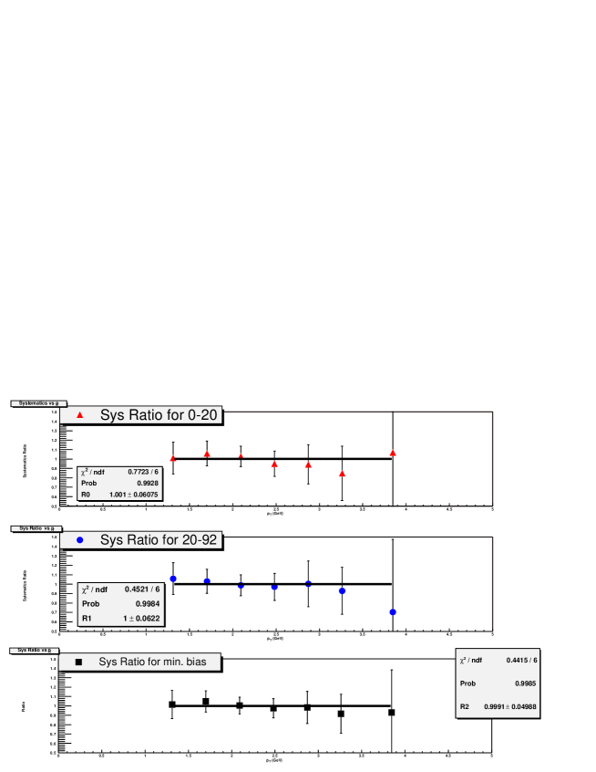
   Figure 4.3: Systematic error estimate for matching cut

2. TOF $E_{loss}$ Systematics: We shifted the $E_{loss}$ cut in the TOF scintillator from $E_{loss}>0.0014\beta^{-5/3}$ GeV to $E_{loss}>0.0016\beta^{-5/3}$ GeV (see Fig. 4.4) to obtain the systematic uncertainty.

   

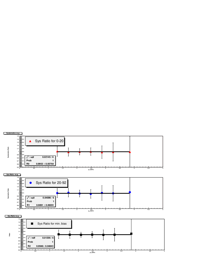
   Figure 4.4: Systematic error estimate for TOF $E_{loss}$ cut

3. PID Systematics:

   In order to estimate the uncertainty in our particle identification (PID) we used three different methods:

   1. The systematic error due to fitting is estimated by comparing the yields from two different functional forms ($1/x$ and $e^{-x}$for the background (see Fig. 4.7).

   2. The binning of the $m^{2}$ histograms is changed to see how it affects the fits (see Fig. 4.5).

   3. The momentum resolution parameters are changed in the fitting routine, to see how it affects the width of $m^{2}$ histograms and hence the fits (see Fig. 4.6).

   

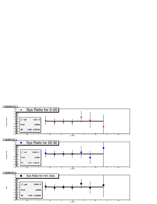
   Figure 4.5: Systematic uncertainty for PID (binning)

   

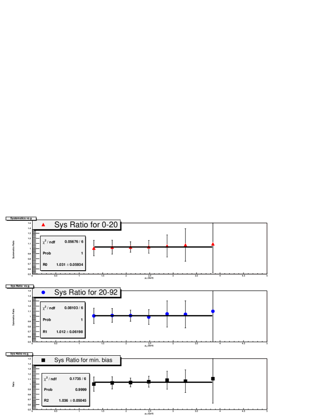
   Figure 4.6: Systematic uncertainty for PID (varying momentum resolution parameters)

   

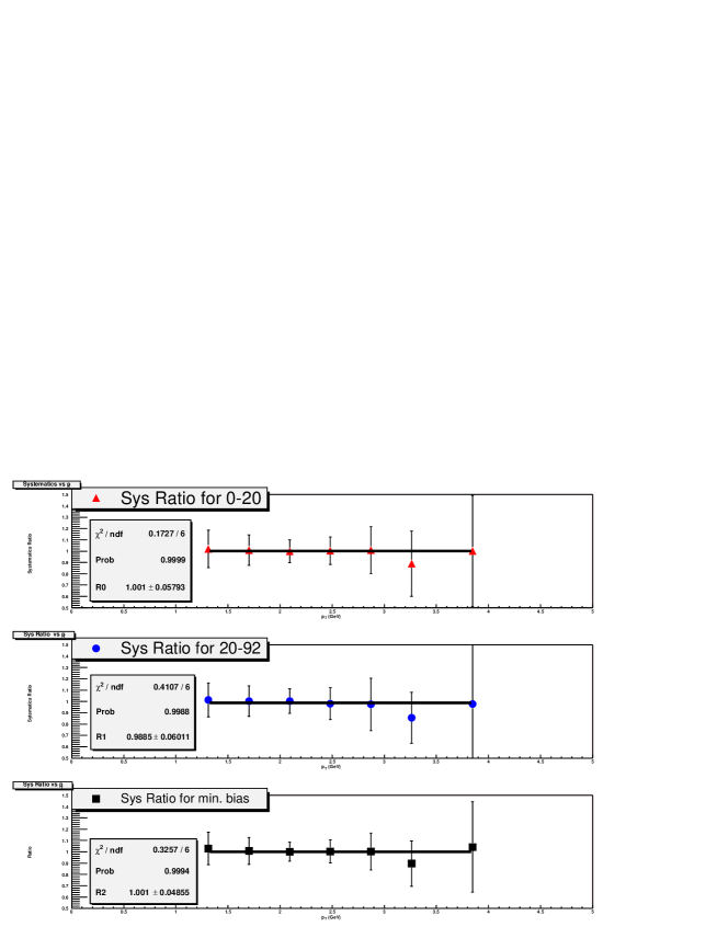
   Figure 4.7: Systematic uncertainty for PID (using $1/x$ function for background instead of $e^{-x}$)

4. Momentum Scale Systematics: The error in our estimate for the momentum scale was found to be 0.71%. This can lead to a systematic uncertainty in our yields that varies as a function of $p_{T}$ reaching $\approx$ 3% at 4.0 GeV (see Fig. 4.8). This was generated by doing a simple Monte Carlo, by generating yields assuming the momentum scale to vary by $\pm$ 0.71%.

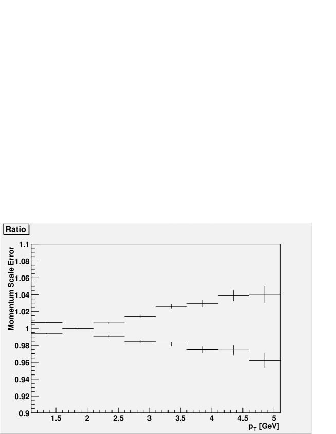
Figure 4.8: Systematic uncertainity due to momentum scale

4.2.2 $p_{T}$ independent systematic uncertainties

Sources of the systematic uncertainties of type II, which are independent of $p_{T}$ are briefly described below:

Table 4.3: $p_{T}$ independent systematic uncertainties from different sources

Centrality	Annihilation $d(\bar{d})$	Embedding	Absolute Normalisation
Min Bias: 0-92%	1.5% (3.5%)	2.74%	2.5%
Most Central: 0-20%	1.5% (3.5%)	7.11%	2.5%
Mid-Central 20-92%	1.5% (3.5%)	3.1%	2.5%

1. Annihilation correction systematics: Systematic uncertainty due to survival (annihilation) correction for deuterons is 1.5% and for anti-deuterons is 3.5%.

2. Embedding correction systematics: As mentioned in the previous chapter, in high multiplicity events, we can lose tracks due to less efficient track reconstruction as well multiple hits in a given detector element. This was corrected for by embedding a simulated event in a real event and running the reconstruction software on it. The uncertainty in this correction is tabulated in Table 3.4.

3. Vertex Dependence: We varied the BBC $z$-vertex from 35 cm to 30 cm and found no change in yields.

4. Absolute normalisation systematics: Small variations in efficiencies of detectors from run to run, can lead to an uncertainty in our absolute normalisation. To determine this we look at the average number of tracks in the TOF (Fig. 4.9), Drift Chamber(Fig. 4.10) and PC3 (Fig. 4.11) from run to run. The variance of this number gives our systematic uncertainty in absolute normalisation ($\approx$ 2.5%).

   

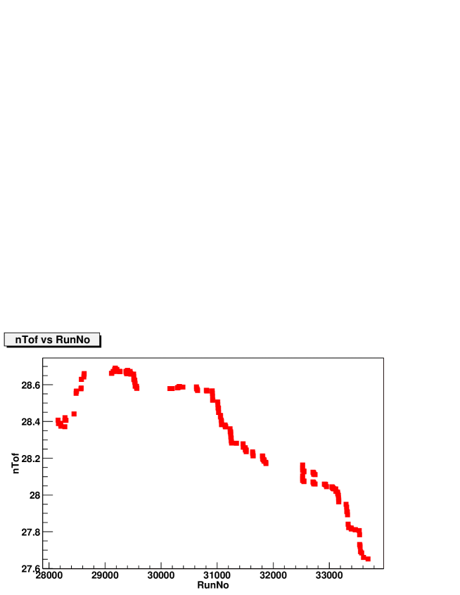
   Figure 4.9: Run by run variation in average number of TOF tracks

   

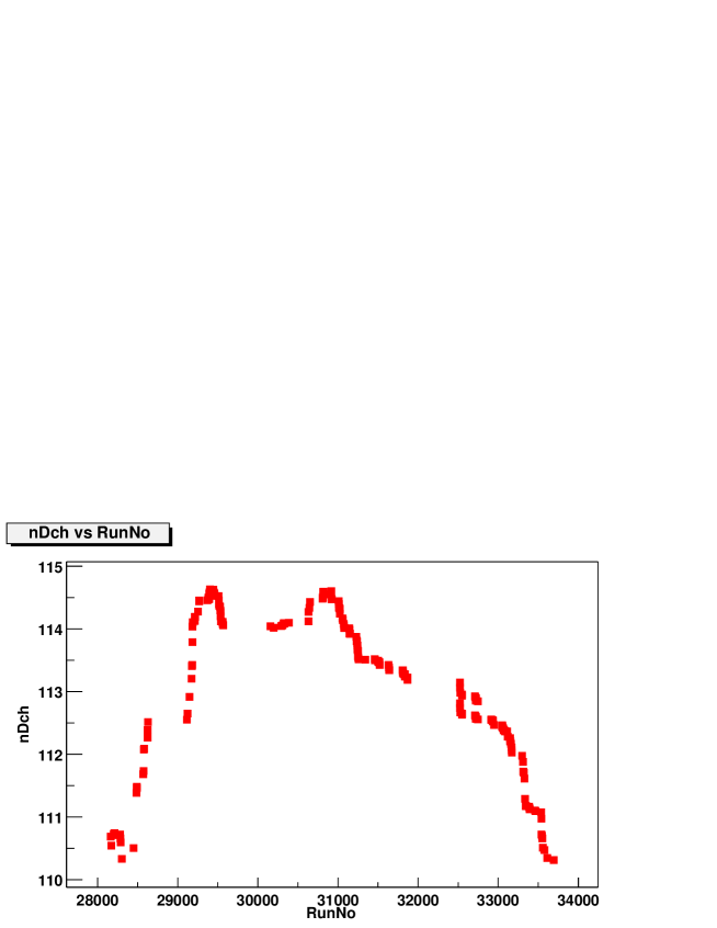
   Figure 4.10: Run by run variation in average number of Drift Chamber tracks

   

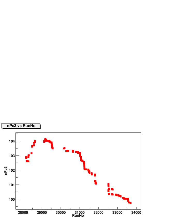
   Figure 4.11: Run by run variation in average number of PC3 tracks

4.3 $\bar{d}/d$ ratios and implications for $\bar{n}/n$ ratio

The $\bar{d}/d$ ratios vs $p_{T}$ are shown in Figures 4.12,  4.13 and 4.14 for different centralities, and the values are listed in Table4.4. The $\bar{d}/d$ ratio does not change as we go from one centrality to the other. We find that $\bar{d}/d=$ 0.47 $\pm$ 0.03 for minbias data. This is consistent with the square of the $\bar{p}/p=0.73\pm 0.01$ [18], within the statistical and the systematic errors, as expected if (anti-)deuterons are formed by coalescence of comoving (anti-)nucleons.

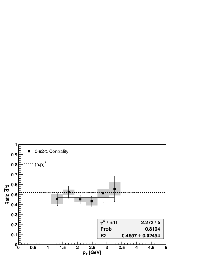
Figure 4.12: $\bar{d}/d$ vs $p_{T}$ for min. bias (grey bars depict systematic uncertainties)

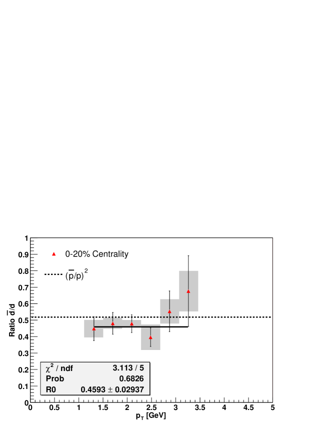
Figure 4.13: $\bar{d}/d$ vs $p_{T}$ for 0-20% most central (grey bars depict systematic uncertainties)

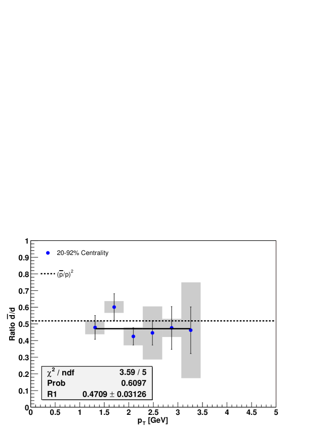
Figure 4.14: $\bar{d}/d$ vs $p_{T}$ for 20-92% mid-central (grey bars depict systematic uncertainties)

The systematic uncertainties were calculated by making same cuts as for the spectra as outlined in previous section, and then taking the $\bar{d}/d$ ratio. For details see Figures 4.15,  4.16, 4.17, 4.18 and 4.19.

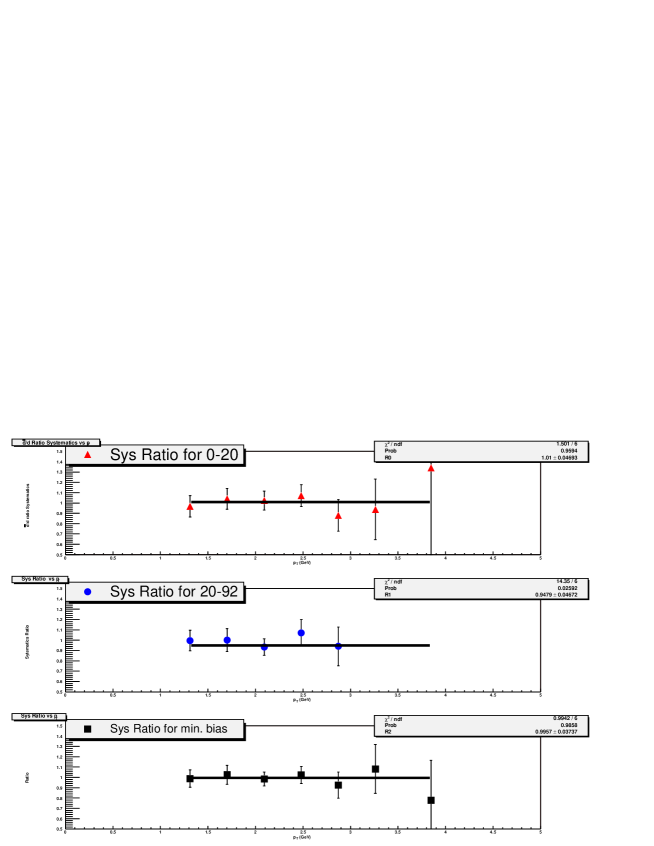
Figure 4.15: $\bar{d}/d$ ratio systematic uncertainty for PID (binning)

Figure 4.16: $\bar{d}/d$ ratio systematic uncertainty for PID (varying momentum resolution parameters)

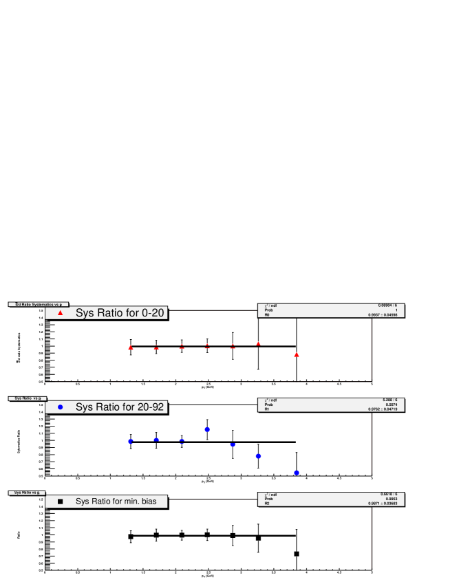
Figure 4.17: $\bar{d}/d$ ratio systematic uncertainty for PID (using $1/x$ function for background instead of $e^{-x}$)

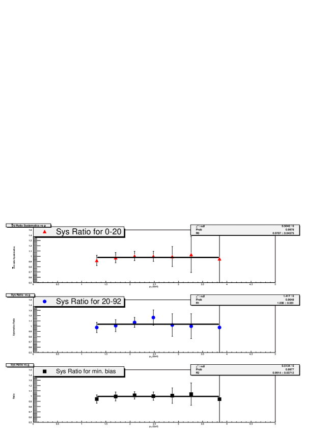
Figure 4.18: $\bar{d}/d$ ratio systematic uncertainty due to Etof cut.

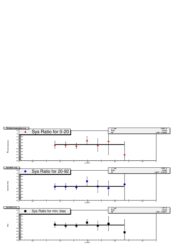
Figure 4.19: $\bar{d}/d$ ratio systematic uncertainty due to matching cuts.

Table 4.4: Values of $\bar{d}/d$ ratio at the mean of each $p_{T}$ bin for different centralities

Centrality	$p_{T}$ [GeV]	$\bar{d}/d$ Ratio	Stat. Errors	Sys. Errors
	1.31193	0.448011	0.0723876	0.0501816
	1.70166	0.480323	0.0661106	0.0284824
	2.09137	0.478307	0.0543533	0.0118666
0-20%	2.48116	0.395729	0.0564264	0.0759096
	2.87113	0.553165	0.123666	0.0709565
	3.26136	0.676205	0.214811	0.120164
	3.83075	0.837902	0.435682	0.389956
	1.31193	0.478774	0.0716046	0.0366907
	1.70166	0.601043	0.0797217	0.0267981
	2.09137	0.424859	0.0518895	0.0511881
20-90%	2.48116	0.44557	0.0729878	0.158388
	2.87113	0.475816	0.128523	0.0509976
	3.26136	0.461791	0.139587	0.286625
	3.83075	0.561234	0.379337	0.448365
	1.31193	0.452872	0.0627106	0.0441257
	1.70166	0.523841	0.0616634	0.0168406
	2.09137	0.449582	0.0424838	0.012414
Min. Bias	2.48116	0.432023	0.0493521	0.0386692
	2.87113	0.510429	0.0921352	0.0406558
	3.26136	0.555987	0.128219	0.0620898
	3.83075	0.849898	0.380574	0.365119

The ratio $\bar{n}/n$ can be estimated from the data based on the thermal chemical model. Assuming thermal and chemical equilibrium, the chemical fugacities are determined from the particle/anti-particle ratios [39]:

$$\frac{E_{A}(d^{3}N_{A}/d^{3}p_{A})}{E_{\bar{A}}(d^{3}N_{\bar{A}}/d^{3}p_{\bar{A}})}=\exp\left(\frac{2\mu_{A}}{T}\right)=\lambda_{A}^{2}$$ (4.1)

Using the ratio $p/\bar{p}$, the extracted proton fugacity is $\lambda_{p}=\exp(\mu_{p}/T)$ = 1.17 $\pm$ 0.01. Similarly, using the $d/\bar{d}$ ratio, the extracted deuteron fugacity is $\lambda_{d}=\exp[(\mu_{p}+\mu_{n})/T]$ = 1.46 $\pm$ 0.05. From this, the neutron fugacity can be estimated to be $\lambda_{n}=\exp(\mu_{n}/T)$ = 1.25 $\pm$ 0.04, which results in $\bar{n}/n$ = 0.64 $\pm$ 0.04. These estimates, along with equality of the coalescence parameter $B_{2}$ (to be discussed in detail in later sections) for $d$ and $\bar{d}$ indicate that, within errors, $\mu_{n}\geq\mu_{p}$. This is expected since the entrance Au+Au channel has larger net neutron density than net proton density. This effect is also seen in the kaon ratio: $K^{-}/K^{+}=0.933\pm 0.007$ [18], which is slightly less than unity. Most particle ratios compare well with the thermal model predictions [41].

4.4 $T_{eff}$, $dN/dy$ and $<p_{T}>$

The $p_{T}$ shapes of the particle spectra an be quantified by looking at the spectral slopes. It has been observed at lower beam energies, that particle invariant yields often exhibit an exponential slope in the transverse mass $m_{T}$. This is parameterized in terms of the inverse slope parameter $T_{eff}$ as follows:

$$\frac{d^{2}N}{2\pi N_{evt}m_{t}dm_{t}dy}=Ae^{-m_{t}/T_{eff}}$$ (4.2)

We fitted the above function to the (anti-)deuteron spectra in the range $1.1<p_{T}<3.5$ GeV/$c$ for different centralities. The fits can be seen Figures 4.20, 4.21, and  4.22. Deuterons are depicted by red squares, whereas anti-deuterons are depicted by blue triangles and the line overlaid on the spectra is the fit. The spectra have a shoulder arm shape characteristic of hydrodynamic flow, which pushes heavier particles to higher $p_{T}$ as a result of interactions. The inverse slopes ($T_{eff}$) of the spectra are tabulated in Table 4.5. The deuteron inverse slopes of $T_{eff}$ = 500–520 MeV are considerably higher than the $T_{eff}$ = 300–350 MeV observed for protons [17, 18]. However, we also observe that our spectra curve downwards at low $p_{T}$ and are not very well described by a simple $m_{T}$. This is indicates that source in the collision zone is not static, but expanding. A more sophisticated treatment incorporating hydrodynamical flow effects was developed by R. Scheibl and U. Heinz  [39].

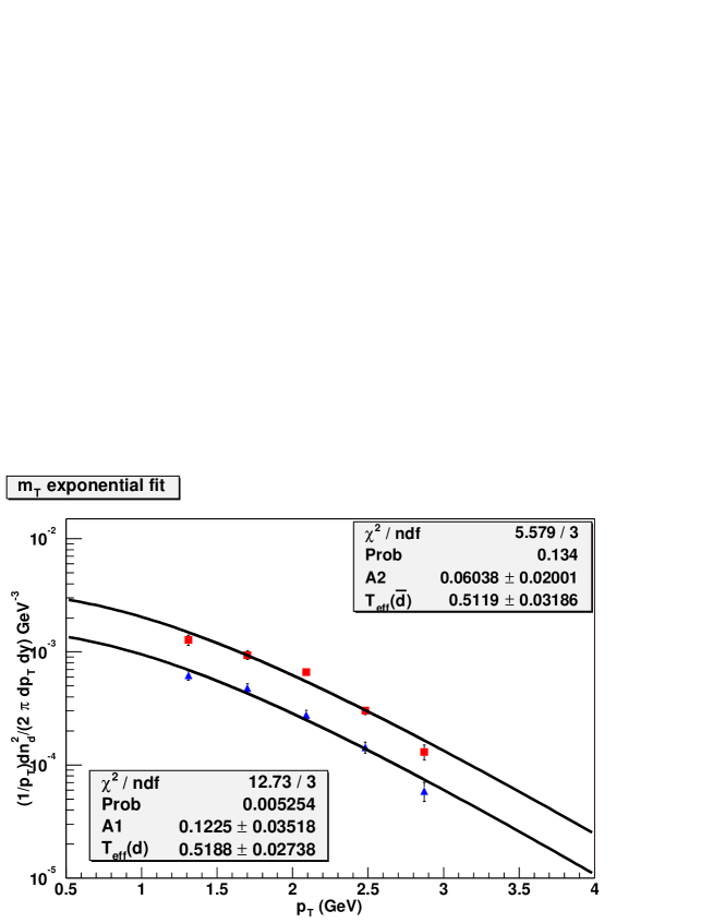
Figure 4.20: $T_{eff}$ fits using a $m_{T}$ exponential for min. bias data.

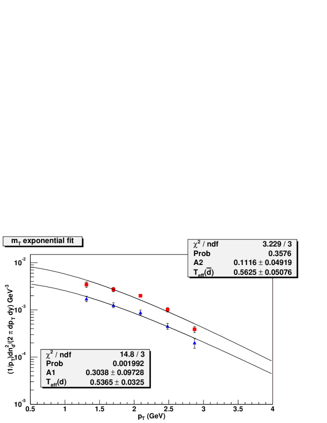
Figure 4.21: $T_{eff}$ fits using a $m_{T}$ exponential for 0-20% centrality.

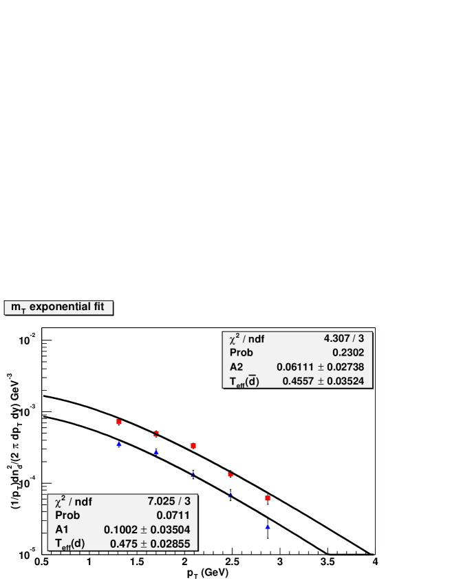
Figure 4.22: $T_{eff}$ fits using a $m_{T}$ exponential for 20-92% centrality.

The invariant yields $dN/dy$ and the average transverse momenta $\langle p_{T}\rangle$ are obtained by summing the data over $p_{T}$ and using a functional form to extrapolate to low $m_{T}$ regions where we have no data. $dN/dy$ was calculated as follows:

$$\frac{dN_{d}}{dy}=\int_{0}^{\infty}2\pi p_{T}f(p_{T})dp_{T}$$ (4.3)

where $f(p_{T})$ is the function that gives us the yield as a function of $p_{T}$:

$$\frac{d^{2}N_{d}}{2\pi dp_{T}dy}=f(p_{T})$$ (4.4)

In order to minimise our errors, we subdivided this integral into three regions:

1. $p_{T}$ in the range 0 – 1.1 GeV (the beginning of our experimental data), where we used an extrapolated function. For the extrapolation function we used a Boltzmann distribution of the form:

   $$\frac{d^{2}n}{2\pi m_{t}dm_{t}dy}=Am_{T}e^{-m_{t}/T_{eff}}$$ (4.5)

   for the extrapolation fit as it gives a slightly better $\chi^{2}/n.d.f.=4.8/3$ vs. $\chi^{2}/n.d.f.=5.6/3$ for $m_{T}$ exponential. The fits are shown in Figures  4.23,  4.24, 4.25).

2. $p_{T}$ in the range 1.1 – 4.3 GeV, for which we numerically integrated our data.

3. $p_{T}$ in the range 4.3 – $\infty$ GeV, where we again extrapolated.

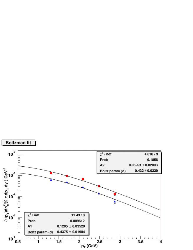
Figure 4.23: Fits using a Boltzmann Distribution for min. bias data.

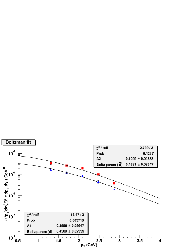
Figure 4.24: Fits using a Boltzmann Distribution for 0-20% centrality.

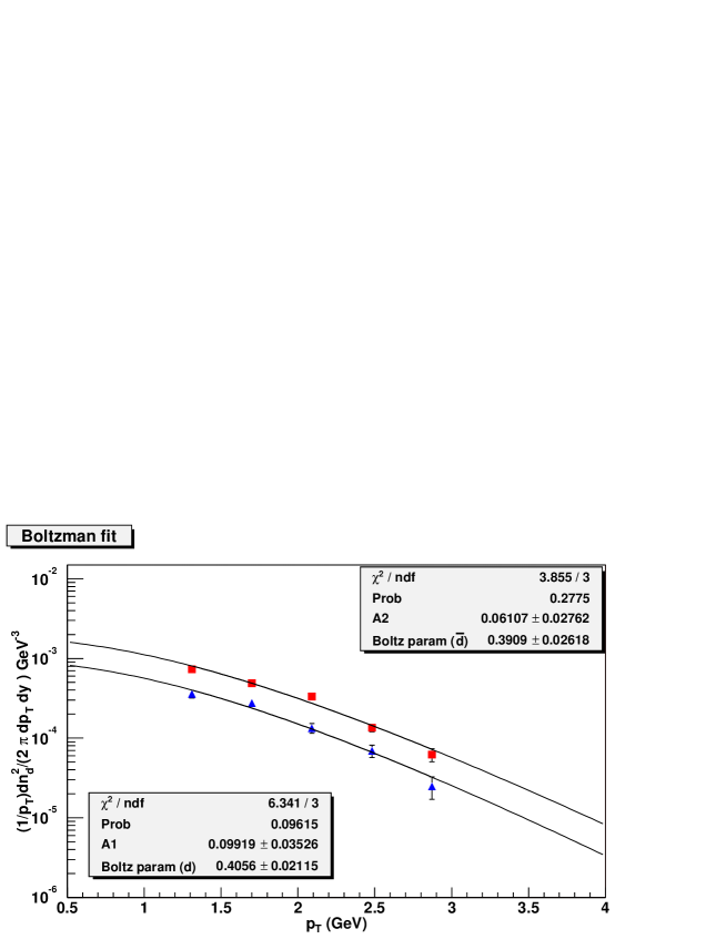
Figure 4.25: Fits using a Boltzmann Distribution for 20-92% centrality.

Table 4.5: The inverse slope parameter $T_{eff}$ obtained from a $m_{T}$ exponential fit to the spectra along with multiplicity $dN/dy$ and mean transverse momentum $\langle p_{T}\rangle$ obtained from a Boltzman distribution for different centralities:

$T_{eff}$ [MeV]	Deuterons	Anti-deuterons
Minimum Bias	519 $\pm$ 27	512 $\pm$ 32
0-20%	536 $\pm$ 32	562 $\pm$ 51
20-92%	475 $\pm$ 29	456 $\pm$ 35
$dN/dy$
Minimum Bias	0.0250 $\pm^{0.0006(stat.)}_{0.005(sys.)}$	0.0117 $\pm^{0.0003(stat.)}_{0.002(sys.)}$
0-20%	0.0727 $\pm^{0.0022(stat.)}_{0.0141(sys.)}$	0.0336 $\pm^{0.0013(stat.)}_{0.0057(sys.)}$
20-92%	0.0133 $\pm^{0.0004(stat.)}_{0.0029(sys.)}$	0.0066 $\pm^{0.0002(stat.)}_{0.0015(sys.)}$
$\langle p_{T}\rangle$ [GeV/$c$]
Minimum Bias	1.54 $\pm^{0.04(stat.)}_{0.13(sys.)}$	1.52 $\pm^{0.05(stat.)}_{0.12(sys.)}$
0-20%	1.58 $\pm^{0.05(stat.)}_{0.13(sys.)}$	1.62 $\pm^{0.07(stat.)}_{0.1(sys.)}$
20-92%	1.45 $\pm^{0.05(stat.)}_{0.15(sys.)}$	1.41 $\pm^{0.06(stat.)}_{0.15(sys.)}$

The extrapolated yields constitute $\approx$ 42% of our total yields. $<p_{T}>$ was obtained in a similar manner, by taking the ratio of integrals:

$$<p_{T}>=\frac{\int_{0}^{\infty}p_{T}^{2}f(p_{T})dp_{T}}{\int_{0}^{\infty}p_{T}f(p_{T})dp_{T}}$$ (4.6)

Systematic uncertainties on $dN/dy$ and $\langle p_{T}\rangle$ are estimated by using an exponential in $p_{T}$ (instead of in $m_{T}$) and a “truncated” Boltzman distribution (assumed flat for $p_{T}<1.1$ GeV/$c$) for alternative extrapolations. Systematic uncertaintiess on $dN/dy$ and $<p_{T}>$ were estimated by using two different functional forms:

1. $p_{T}$ exponential fit, of the form:

   $$\frac{d^{2}n}{2\pi m_{t}dm_{t}dy}=Ae^{-p_{t}/T_{const.}}$$ (4.7)

   The $p_{T}$ exponential fits are shown in Figures 4.26, 4.27, 4.28.

   

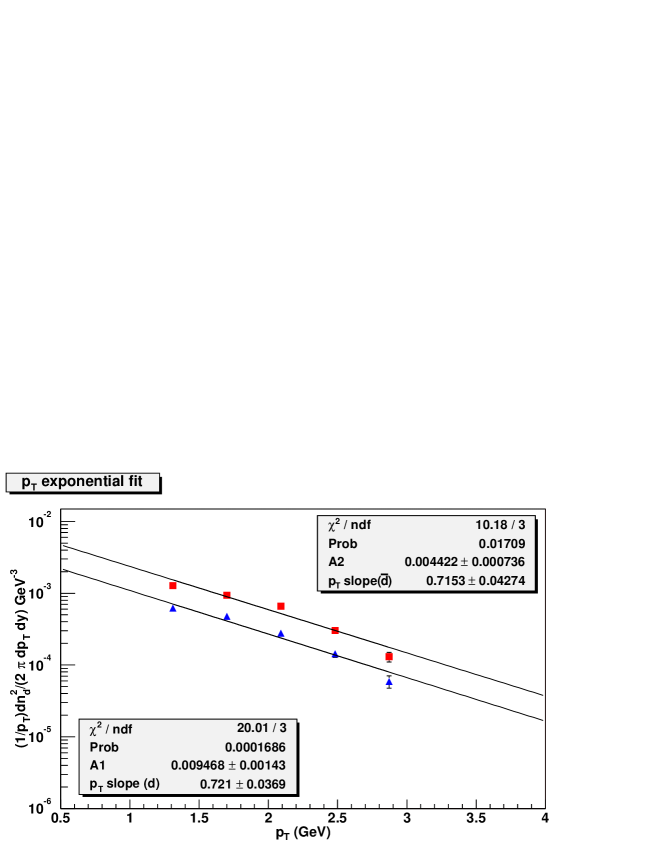
   Figure 4.26: Fits using a $p_{T}$ exponential for min. bias data.

   

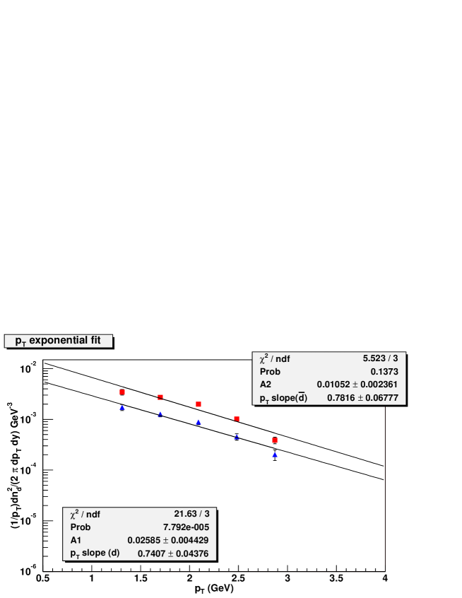
   Figure 4.27: Fits using a $p_{T}$ exponential for 0-20% centrality.

   

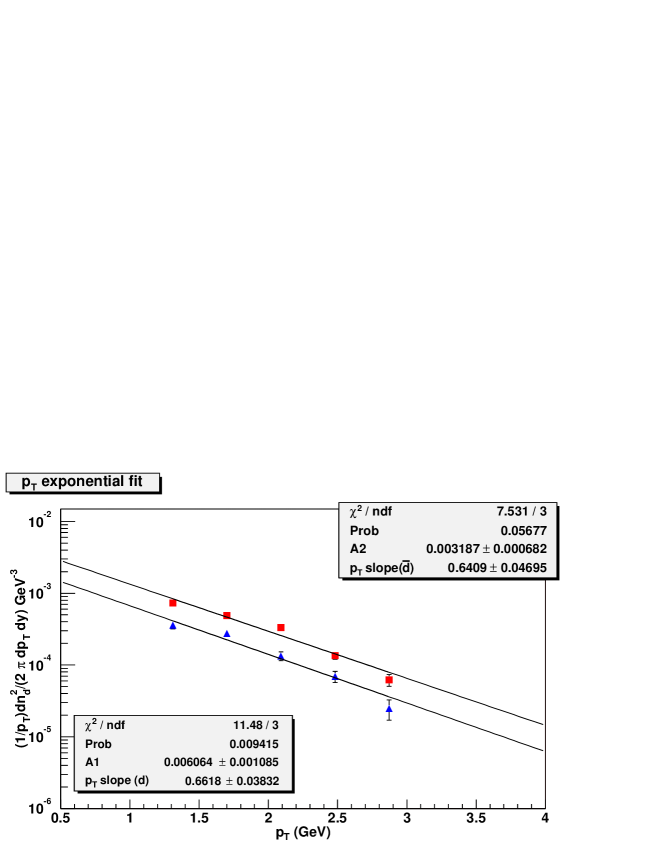
   Figure 4.28: Fits using a $p_{T}$ exponential for 20-92% centrality.

2. Truncated Boltzmann fit, in which we assume a flat distribution for $p_{T}<1.1$ GeV (see Figures 4.29, 4.30,  4.31):

   

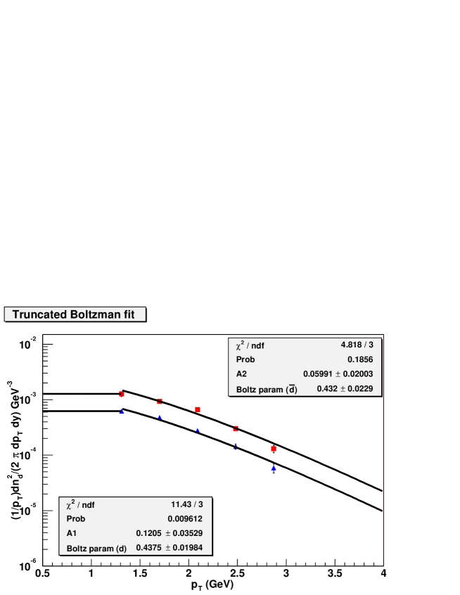
   Figure 4.29: Fits using a Truncated Boltzmann Distribution for min. bias data.

   

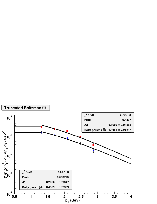
   Figure 4.30: Fits using a Truncated Boltzmann Distribution for 0-20% centrality.

   

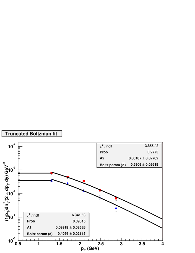
   Figure 4.31: Fits using a Truncated Boltzmann Distribution for 20-92% centrality.

The inverse slope parameter $T_{eff}$, rapidity distributions $dN/dy$, and the mean transverse momenta $\langle p_{T}\rangle$, are compiled in Table 4.5 for three different centrality bins.

4.5 Coalescence parameter $B_{2}$

With a binding energy of 2.24 MeV, the deuteron is a very loosely bound state. Thus, it is formed only at a later stage in the collision, most likely after elastic hadronic interactions have ceased; the proton and neutron must be close in space and tightly correlated in velocity to coalesce. As a result, $d$ and $\bar{d}$ yields are a sensitive measure of correlations in phase space and can provide information about the space-time evolution of the system. If deuterons are formed by coalescence of protons and neutrons, the invariant deuteron yield can be related [42] to the primordial nucleon yields by:

$$E_{d}\frac{d^{3}N_{d}}{d^{3}p_{d}}\biggr{|}_{p_{d}=2p_{p}}=B_{2}\left(E_{p}\frac{d^{3}N_{p}}{d^{3}p_{p}}\right)^{2}$$ (4.8)

where $B_{2}$ is the coalescence parameter, with the subscript implying that two nucleons are involved in the coalescence. The above equation includes an implicit assumption that the ratio of neutrons to protons is unity. The proton and antiproton spectra [18] are corrected for feed-down from $\Lambda$ and $\bar{\Lambda}$ decays by using a MC simulation tuned to reproduce the particle ratios: ($\Lambda/p$ and $\bar{\Lambda}/\bar{p}$) measured by PHENIX at 130 GeV [34].

We calculated $B_{2}$ by taking the scaled ratio of the deuteron and anti-deuteron spectra with the square of the spectra of the proton and anti-proton spectra, for each $p_{T}$ bin in comparable centralities. The data for the proton and anti-proton spectra was taken from published PHENIX papers [18]. Systematical uncertainties are mostly same as for the $d$, $\bar{d}$ spectra, except that the $p$, $\bar{p}$ spectra have an additional uncertainty due to feeding down from $\Lambda$, $\bar{\Lambda}$ decays, which leads to an uncertainty of 10.2% in $B_{2}$.

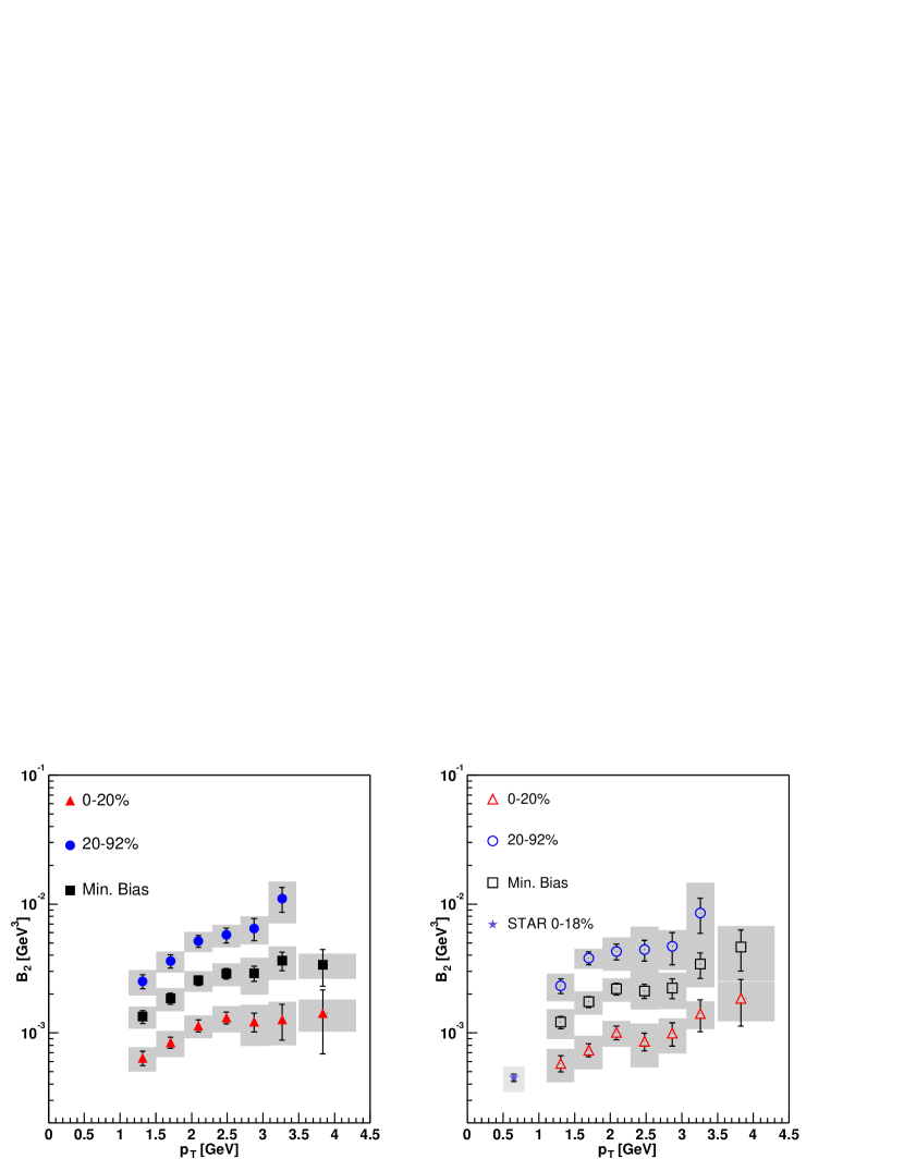
Figure 4.32: Coalescence parameter $B_{2}$ vs $p_{T}$ for deuterons (left panel) and anti-deuterons (right panel). Grey bands indicate the systematic errors. Values are plotted at the “true” mean value of $p_{T}$ of each bin, the extent of which is indicated by the width of the grey bars along x-axis.

Figure 4.32 displays the coalescence parameter $B_{2}$ as a function of $p_{T}$ for different centralities (the values are given in Table 4.6). We notice some important trends:

Table 4.6: Coalescence parameter $B_{2}$ for different centralities

Centrality	$p_{T}$ [GeV]	$B_{2}$ [GeV2/c3] (deuterons)	$\bar{B_{2}}$ [GeV2/c3] (anti-deuterons)
	1.31193	0.000639055 $\pm$ 7.50E-05	0.000581546 $\pm$ 8.32E-05
	1.70166	0.000843443 $\pm$ 8.91E-05	0.000736467 $\pm$ 8.50E-05
	2.09137	0.00113993 $\pm$ 9.86E-05	0.00100924 $\pm$ 0.000121727
0-20%	2.48116	0.00131118 $\pm$ 0.000132695	0.000862111 $\pm$ 0.000137338
	2.87113	0.00122166 $\pm$ 0.000192384	0.00099636 $\pm$ 0.000203503
	3.26136	0.00127308 $\pm$ 0.000279434	0.00141501 $\pm$ 0.000393006
	3.83075	0.00141949 $\pm$ 0.000521348	0.00185868 $\pm$ 0.000731906
	1.31193	0.00251278 $\pm$ 0.000315446	0.00232644 $\pm$ 0.000304454
	1.70166	0.00361427 $\pm$ 0.000426224	0.00381079 $\pm$ 0.00044324
	2.09137	0.00514855 $\pm$ 0.000552146	0.00427978 $\pm$ 0.000604291
20-90%	2.48116	0.00574697 $\pm$ 0.000756338	0.00442243 $\pm$ 0.000807512
	2.87113	0.00644265 $\pm$ 0.00124428	0.00469217 $\pm$ 0.0013238
	3.26136	0.0109891 $\pm$ 0.00239219	0.00849642 $\pm$ 0.002594
	3.83075	0.00950758 $\pm$ 0.00417112	0.00858541 $\pm$ 0.00581748
	1.31193	0.00133957 $\pm$ 0.000153907	0.00121209 $\pm$ 0.000132676
	1.70166	0.00185072 $\pm$ 0.000187566	0.0017466 $\pm$ 0.000174225
	2.09137	0.00255682 $\pm$ 0.000216065	0.00219478 $\pm$ 0.00023407
Min. Bias.	2.48116	0.00288005 $\pm$ 0.000275283	0.00211784 $\pm$ 0.000267098
	2.87113	0.00290036 $\pm$ 0.000386863	0.00223415 $\pm$ 0.000397725
	3.26136	0.00364134 $\pm$ 0.000592348	0.00341505 $\pm$ 0.000760932
	3.83075	0.00336927 $\pm$ 0.00105975	0.00463725 $\pm$ 0.00162501

1. The decreased $B_{2}$ in more central collisions implies that in larger sources, the average relative separation between nucleons increases, thus decreasing the probability of formation of deuterons.

2. We observe that $B_{2}$ increases with $p_{T}$. This is consistent with an expanding source because position-momentum correlations lead to a higher coalescence probability at larger $p_{T}$. The $p_{T}$-dependence of $B_{2}$ can also provide information about the density profile of the source as well as the expansion velocity distribution. It has been shown [39, 40] that generally a Gaussian source density profile leads to a constant $B_{2}$ with $p_{T}$ as it gives greater weight to the center of the system, where radial expansion is weakest. This is not supported by our data, which shows a rise in $B_{2}$ with $p_{T}$.

   

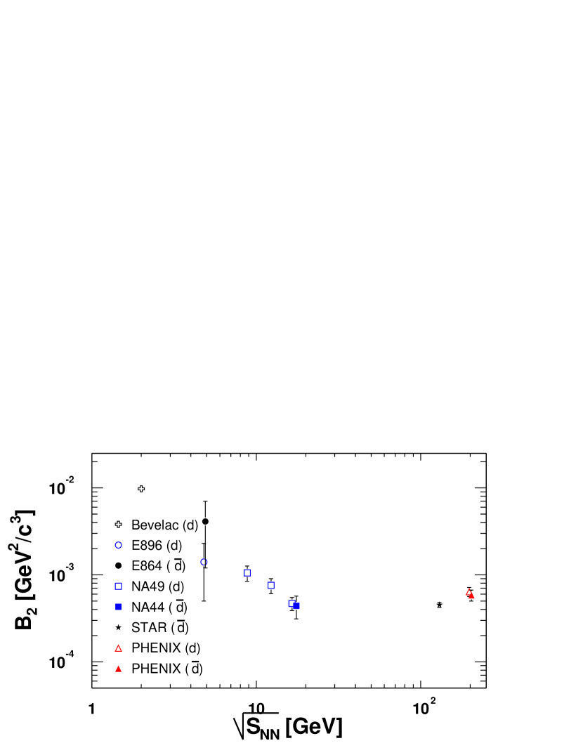
   Figure 4.33: (color online) Comparison of the coalescence parameter for deuterons and anti-deuterons ($p_{T}$ = 1.3 GeV/$c$) with other experiments at different values of $\sqrt{s}$.

3. Figure 4.33 compares $B_{2}$ for most central collisions to results at lower $\sqrt{s}$ [43, 44, 45, 46, 47, 48]. Note that $B_{2}$ is nearly independent of $\sqrt{s}$, indicating that the source volume does not change appreciably with center-of-mass energy (with the caveat that $B_{2}$ varies as a function of $p_{T}$, centrality and rapidity). Similar behavior is seen for $B_{2}$ for deuterons [46] as a function of $\sqrt{s}$. This observation is consistent with what has been observed in Bose-Einstein correlation Hanbury-Brown Twiss (HBT) analysis at RHIC [49, 50] for identified particles. The coalescence parameter $B_{2}$ for $d$ and $\bar{d}$, is equal within errors, indicating that nucleons and antinucleons have the same temperature, flow and freeze-out density distributions.

4. Thermodynamic models [16] predict that $B_{2}$ scales with the inverse of the effective volume $V_{eff}$ ($B_{2}\propto 1/V_{eff}$). $d$ and $\bar{d}$ spectra are affected by radial flow, which concentrates the coalescing protons and neutrons, affecting phase space correlations, thereby limiting the applicability of a simple thermodynamical model to determine an effective source size. $B_{2}$ can also be used to obtain a source radius, analogous to a two particle Bose-Einstein correlation [39] measurement. Although the “correct” physical interpretation of $B_{2}$ is still sometimes debated, thermodynamic models can be used to extract the radius of the source from $B_{2}$, albeit in a model dependent way. For a fireball model in thermal and chemical equilibrium [15, 16], the following relation holds:

   $$R^{3}=\alpha R_{np}(\hbar c)^{3}\frac{m_{d}}{m_{p}^{2}}B_{2}^{-1}$$ (4.9)

   where $\alpha=(3/4)\pi^{3/2}$ for a gaussian source and and $\alpha=(9/2)\pi^{2}$ for a hard sphere and $R_{np}$ is the ratio of neutrons to protons (assumed to be unity here). Assuming a gaussian distributed particle source, we find $R=4.9\pm 0.2$ fm for the $0-20\%$ most central collisons for deuterons at $p_{T}$ = 1.3 GeV (equivalent to proton momentum of $p_{p}$ = 0.65 GeV). It should be noted that deuteron spectra are affected by radial flow, which concentrates the coalescing protons and neutrons, affecting phase space correlations and limiting the applicability of the simple Eq. 4.9.

5. The coalescence parameter $B_{2}$ for $d$ and $\bar{d}$, is equal within errors, indicating that nucleons and antinucleons have the same temperature, flow and freeze-out density distributions. This, alongwith the values of $\bar{d}/d$ ratios indicate that, within errors, $\mu_{n}\geq\mu_{p}$. This is expected since the entrance Au+Au channel has larger net neutron density than net proton density.

Chapter 5 Nuclear modification factor and the initial conditions

In the previous chapters, by looking at the yields of deuterons and anti-deuterons, formed from the dense system of particles from the collision zone, as it expanded and cooled, we were able study the final state effects in Ultra Relativistic Heavy Ion Collisions of Au+Au nuclei at $\sqrt{s_{NN}}=200$ GeV. In this chapter we shift to the second part of this thesis: studying the initial state effects using hadronic probes.

5.1 Parton Distribution Functions

In the 1960s, scattering experiments were conducted at the Stanford Linear Accelerator Center (SLAC) in which very high energy electron beams were fired on protons. This experiment was similar to Rutherford’s classic experiment of bombarding a thin gold foil with $\alpha$-particles, which revealed that the atom consisted of a small massive nucleus, which had most of the atom’s positive charge, and was surrounded by a cloud of electrons. The SLAC experiments found that more electrons were scattered with large momentum transfers than expected. This indicated the presence of discrete scattering centers inside the proton, very much the same way large scattering angles of the $\alpha$-particles indicated the existence of a small and massive nucleus. Moreover, the distribution of the scattering data showed ‘scale-invariance’, which indicated that these scattering centers were ‘point-like’ i.e., they did not have any substructure (at least at the energy scale they were being probed). These were given the generic name: partons. This lead to the developement of the parton model by Feynman [51] (and also by Bjorken and Paschos [52]), in which the nucleon was envisaged to consist of essentially free point-like constituents, the “partons”, from which the electron scatters incoherently. At a more quantitative level they also introduced the concept of parton distributions $q_{i}(x)$, which measure the probability of finding a parton of type $i$ in the proton, with a momentum fraction $x$ of the proton momentum. In the parton model, these parton distributions are independent of the energy scale at which the proton is being probed. The data also indicated that the charged scattering centers were spin $\frac{1}{2}$ fermions. Subsequently, they were identified with the quarks proposed by Murray Gell-Man [53]. Later experiments with neutrinos also supported this view. Parton distributions (PDFs) are essential for a detailed understanding of the nucleon structure as well as experiments involving hadronic initial states, and they evolve as one goes from one momentum scale (or equivalently length scale) to another. From a given initial distribution, it is possible to calculate the evolution of PDFs using the framework of the DGLAP evolution equations [54]. The partons in the nucleon are either:

• Valence quarks: $u,d$-quarks usually with large momentum fractions. Valence parton distribution functions (PDFs) peak around 1/3 and go to zero at momentum fraction of $x$ of 0. A typical PDF for valence quarks at $Q^{2}=100$ GeV shown in Figure 5.1.

• Sea partons consisting of gluons, and quark-antiquark pairs. These usually have a softer distribution and diverge at small-$x$. A typical PDF for gluons at $Q^{2}=100$ GeV shown in Figure 5.2. This increase in gluon density has been observed at HERA [55] for high $Q^{2}$ (momentum transfer) and small-$x$.

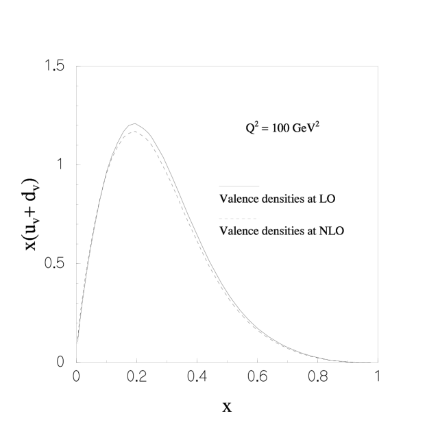
Figure 5.1: A typical parton distribution function (PDF) for valence quarks at $Q^{2}=100$ GeV.

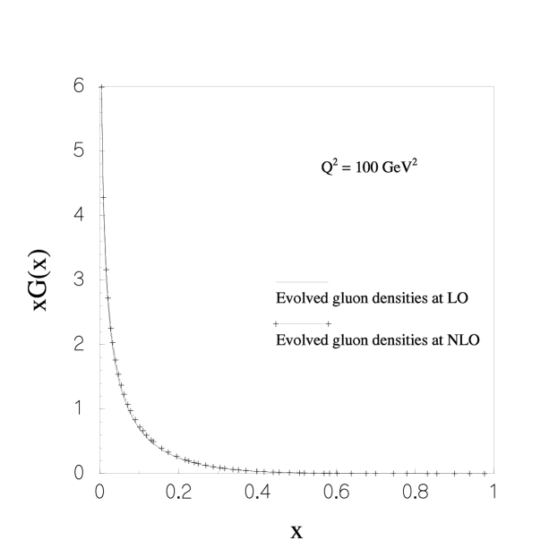
Figure 5.2: A typical PDF for gluons at $Q^{2}=100$ GeV.

5.2 Hard Scattering

In high energy collisions hard scatterings can produce jets of particles. A schematic depiction of jet production via hard scattering is shown in Figure 5.3. The production of energetic high $p_{T}$ particles depends on the distribution of the scattering centers i.e., quarks (valence and sea) and gluons. As a result study of jet production can shed light into PDFs.

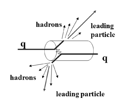
Figure 5.3: A schematic depiction of jet production through hard scattering.

In previous section we saw how the gluon (and sea quark) PDFs diverge at small-$x$. However, this seems to be contrary to needs of unitarity principle. The non-Abelian nature of QCD and the fact that gluons themselves carry color “charge” can lead to gluon fusion processes of type $g+g\rightarrow g$. This can lead to the depletion of the small-$x$ partons in a nucleus compared to those in a nucleon. This phenomenon is known as shadowing [56]. Naively shadowing can be understood from the uncertainty principle: small-$x$ quarks and gluons can spread over a distance comparable to the nucleon-nucleon separation, leading to a spatial overlap and fusion. The depletes the number of partons in small-$x$ region (shadowing) and increasing the density of high momentum partons (anti-shadowing). The increasing gluon fusion processes at small-$x$ can lead the gluon PDFs to stop increasing (gluon saturation). The Color Glass Condensate theory [25] gives a universal QCD explanation for the low-$x$ shadowing.

5.3 Nuclear modification factor: $R_{cp}$

An experimentally simple and convenient way to study particle production is to look at the ratio $R_{cp}$ of the particle yield in central collisions with the particle yield in peripheral collisions, each normalized by number of nucleon nucleon inelastic scatterings ($N_{coll}$). Also known as the nuclear modification factor, $R_{cp}$ is defined as:

$$R_{cp}=\frac{\left(\frac{dN}{d\sigma dp_{T}}\right)^{Central}/N_{coll}^{Central}}{\left(\frac{dN}{d\sigma dp_{T}}\right)^{Peripheral}/N_{coll}^{Peripheral}}$$ (5.1)

A Glauber model [57] and BBC simulation was used to obtain $N_{coll}$. $R_{cp}$ is what we get divided by what we expect. If particle production in Heavy Ion Collisions was simply an incoherent sum of p+p collisions, then $R_{cp}$ would be unity. Any deviation from unity would indicate a different kind of physics. Thus, we assume that peripheral collisions are similar to p+p collisions, allowing us to normalise $R_{cp}$ independent of the p+p reference spectrum. As a result many systematics related to detector efficiencies cancel, leading to a relatively clean measurement with minimal systematics.

Measurement of the $R_{cp}$ variable, has yielded some of the most interesting results at RHIC. At mid-rapidity, $R_{cp}$ was observed to be suppressed at Au + Au collisions at $\sqrt{s_{NN}}=200$ GeV [19, 20, 21, 22]. This could be explained in either in terms of:

1. Jet Suppression: energy loss of energetic particles due to dense partonic matter formed as a result of deconfinement. This energy loss $\simeq$ GeV/fm, and is mostly due to gluon bremmstrahlung processes. This results in a decrease in the yield of high energy particles or jet suppression [58, 59, 9]. This would be mean that the observed suppression in Au+Au collisions at RHIC is a final state effect.

2. Color Glass Condensate (CGC) [25, 26, 27]: at sufficiently high energies and low $x$-values (momentum fraction of nucleon carried by the parton) gluon fusion processes can deplete the number of scattering centers. This can lead to lower particle multiplicities and hence suppression in $R_{cp}$. This would mean that the observed suppression is an initial state effect.

In order to determine whether the observed suppression in $R_{cp}$ was due to initial state effects (CGC or gluon saturation) or due to final state effects (deconfinement leading to jet suppression) a control experiment was performed at RHIC, using deuteron on gold collisions at the same energy $\sqrt{s}=200$ GeV. By comparing results from d+Au collisions with those from Au+Au collisions we can attempt to distinguish between effects that could potentially be due to deconfinement, versus effects of cold nuclear matter. No suppression in $R_{cp}$ was observed in the d+Au collisions at mid-rapidity [23], instead an enhancement was observed. This seems to indicate that that the observed suppression at mid-rapidity in Au+Au collisions was likely due to final state effects. This enhancement is referred to as Cronin effect and is theorized to be a result of initial state multiple scattering of the partons.

5.4 $R_{cp}$ and rapidity

Although the d+Au results seem to be inconsistent with the CGC hypothesis, there is a possibility that the saturation effects might be observable at forward and backward rapidities at RHIC. It turns out that a new regime of parton physics at small-$x$ can be reached by going to large rapidities. By looking at $R_{cp}$ at forward (and backward) rapidities we can probe momentum fraction $x$, which can be related to the rapidity and tranvese energy of the particle by the following relations:

$$x=\frac{M_{T}}{\sqrt{s}}e^{-y}$$ (5.2)

$$x=\frac{M_{T}}{\sqrt{s}}e^{y}$$ (5.3)

Due to their forward and backward rapidity coverages, the PHENIX Muon Arms (described in more detail in the next chapter) can be used to probe regimes of both small and large-$x$. The North Arm (d going direction) probes low-$x$ partons from the Au nucleus, allowing us to probe the saturation/shadowing region, while the South Arm (Au going direction) probes high-$x$ partons from Au, allowing us to study the anti-shadowing/Cronin regime.

Our present analysis seeks to extend the $R_{cp}$ measurement for charged hadrons to forward rapidity (approximate pseudorapidity range $1.2<\eta<2.0$) using the Phenix Muon Arms. Any variation of $R_{cp}$ from Deuteron going side to the gold going side from the nominal value of unity would have important implications. Naively one would expect $R_{cp}$ at forward rapidities to behave not very differently from mid-rapidity and show a Cronin enhancement for both Gold going direction and for the Deuteron going direction with a slightly greater increase in the Deuteron going direction. However, shadowing effects at small-$x$ (where $x$ is the fraction of the nucleon momentum carried by the parton) could lead to a suppression on the Deuteron going side. CGC hypothesis too, would lead to a decrease in the number of scattering centers causing suppression. Hence, in order to get a deeper understanding of the perennial interplay between Cronin-like enhancements due to multiple scattering and depletion of scattering centers due to shadowing-like effects, we need to measure $R_{cp}$ at forward and backward rapidities.

Chapter 6 Hadron identification using Muon Arms

6.1 PHENIX Muon Arms

The PHENIX detector has two muon arms: North and South. South Muon Arm acceptance covers from -2.2 to -1.2 in pseudo-rapidity $\eta$ and full azimuth, whereas the North Muon Arm acceptance covers from 1.2 to 2.4 in $\eta$ and full azimuthal acceptance. Each arm is designed to track and identify muons, while rejecting pions and kaons of the order of $\approx 10^{-3}$. Each muon arm is a radial magnetic field spectrometer with a muon tracker (MuTr) and a muon identifier (MuID) consisting of layers of absorber and tracking. In addition, the pole tips of the Central Magnet (CM) made of steel and brass, in the apertures of the muon north and south arms, act as hadron absorbers to reject pions and kaons. The MuTr consists of three stations of cathode-strip readout tracking chambers mounted inside conical-shaped muon magnets. For an illustrative sketch see Figure 6.1.

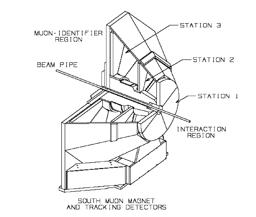
Figure 6.1: The Muon South Arm: muons from the collision point, travel into the Station 1 and so on, eventually reaching the MuID plates behind(not shown in this figure).

The Station 1 tracking chambers are located closest to the interaction region and therefore are the smallest (approximately 1.25 m from inside radius to outside radius), and have the highest occupancy per strip. This also leads to a stringent requirement of a minimum of 95% active area within the acceptance. Station 3 is the last chamber before the MuID and is 2.4 m long and 2.4 m wide. The chamber uses a gas mixture comprising of $50\%Ar+30\%CO_{2}+20\%CF_{4}$ and operates a typical high voltage (HV) of 1850 V, with a gain of $\approx 2\times 10^{4}$. A minimum ionizing particle (MIP) is assumed to deposit 100 electrons, which leads to a total cathode charge of 80 fC. In order to maintain a good momentum resolution down to 1.5 GeV/$c$, the thickness at the Station 2 detector was required to be $\leq 0.1\%$ of a radiation length. This was done by making the Station 2 cathodes (in octant shape) of etched 25 micron copper coated mylar foils.

A track measured in MuTr is identified as a muon if it hits the MuID. A side view of the Muon Arms is shown in Figure 6.2. To reject pions of upto 4 GeV/$c$, steel of depth 90 cm (5.4 hadronic interaction lengths) is required. Since the muon magnet backplate is 30 cm, we need an additional 60 cm in the MuID. This is implemented by segmenting the absorber into 4 layers of thicknesses 10, 10, 20 and 20 cm. This type of segmentation can improve the measurement of trajectories in the MuID. The 5 gaps between the steel segments are instrumented with Iarocci tubes, which are planar drift tubes consisting of 100 $\mu$m gold-coated CuBe anode wires at the center of long channels of a graphite-coated plastic cathode. Groups of Iarocci tubes are arrayed in $x$ and $y$ directions. The MuID for the South Arm is same as the North Arm, except that the Muon Magnet backplate is 20 cm instead of 30 cm in the North Arm.

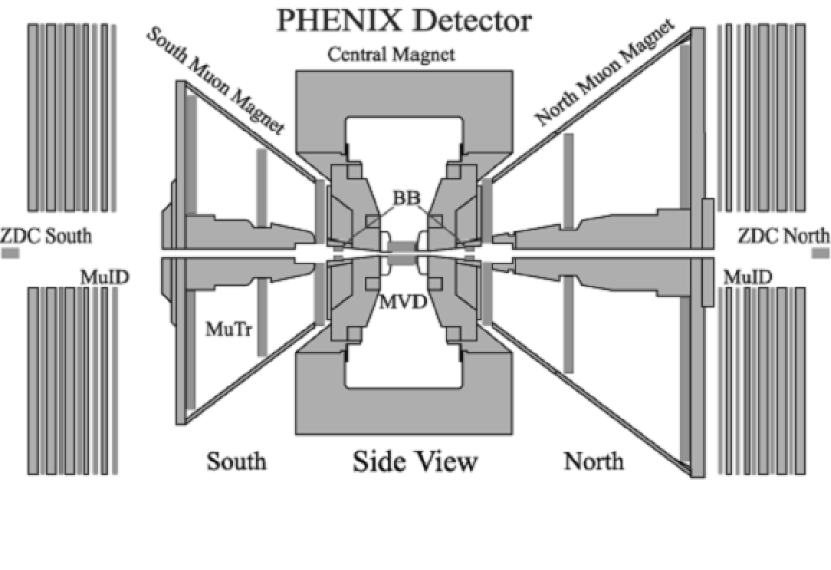
Figure 6.2: A side view of the muon arms shows the muon tracker (MuTr) and the muon identifier (MuID). Particles travel from the collision point, through the muon magnet absorber into the MuTr and finally into the MuID.

6.2 Selection of hadrons

Although the PHENIX Muon Arm Spectrometers [28, 60] were designed to detect muons, we use them in this analysis to measure charged hadrons by rejecting muons: “One man’s meat (hadrons) is another man’s poison (muons)”. Although both muons and hadrons lose their energy when passing through materials via Bethe-Bloch ionization energy loss [30], hadrons can lose a much larger portion of their energy due to hadronic interactions. As mentioned earlier, the PHENIX Muon Arms consist of a tracker (MuTr) with a steel copper absorber in front of the tracker to reduce hadronic background and get better a muon signal (See Figures 6.1 and 6.2). This is followed by layers of the identifier (MuID), which are interleaved with steel plates again to reduce hadronic background. This means that if a particle penetrates to the deepest MuID gap, without getting absorbed in between it was probably a muon, whereas if it stops in the shallow gaps, it is more likely to be a hadron. If we look at the distribution of the total momentum $p_{tot}$ as measured at Station 1  (behind the absorber) stopped at given shallow MuID gaps, (Fig. 6.3) we see that there is a peak of mostly slow muons around 1.3 GeV, and a longer hadronic tail. This is similar to what is seen in Monte Carlo (MC) simulations [61]. Thus, by applying appropriate cuts in $p_{tot}$ and MuID depth, we can identify hadrons.

Figure 6.3: Histogram of momentum measured at station 1 of MuTr for tracks stopping at different MuID gaps from d+Au min. bias data. Around 1.3 GeV there is a peak of mostly stopped muons, followed by a long hadronic tail.

As described previously, the raw data from a run is reconstructed and then saved in easily digestible format, based on detector subsystems or physics type. For this analysis, we used PHENIX Muon nanodsts (MwDSTs), which contain information from the PHENIX Muon Arms. As in previous run, the Zero Degree Calorimeters (ZDCs) and the Beam Beam Counters (BBCs) were used to determine the event centrality (or impact parameter) by looking at multiplicities. For this analysis, we used Minimum Bias (MB) events, which are essentially minimally triggered events in which the BBC and the ZDC fired and are as unbiased as can be made. The event vertex was restricted to $|z|<35$ cm of the collision vertex, primarily for reasons to do with detector acceptances.

After excluding events rejected by our global cuts, we analysed 67 million events. In order to select hadrons we fitted a Gaussian to the peak on Fig. 6.3 and obtained a width of 200 MeV/$c$, centered at 1.3 GeV/$c$. In addition, tracks were selected for optimal signal to background ratio, by using the following cuts:

• Number of hits in the tracker MuTr: $nhits>=12$.

• Track stopping at MuID gap = 2 or 3, exclusively. Since particles that penetrate deeper into the MuID, without stopping in the intervening steel are more likely to be muons, we select only those which stop exclusively in the shallow gaps.

• Total momentum $p_{tot}$(Station 1) $>1.3+3\times 0.2$ = 1.9 GeV/$c$. Since the slow muons (stopped at the shallow gaps) peak around $p_{tot}$ = 1.3 GeV/$c$, we can reject them by excluding particles in that range.

• Track $\chi^{2}<10$ (helps in rejection of ghost tracks).

• $-2.0<\eta<-1.3$ for South Arm and $2.2>\eta>1.3$ for North Arm. These acceptance cuts are applied to reduce the small angle background, mainly from beam gas interactions.

6.3 Sources of contamination

We have two main sources of contamination:

1. Muon contamination through prompt muons (which are produced at the collision point) and muons from meson decays.

2. Hadronic showers.

Most muons are produced through meson decays, primarily pions and kaons. Although most pions and kaons produced in the collision are stopped at the absorber, some decay into muons along their flight path. As a result, the further the collision vertex is from the absorber greater is the probability that the pion (or kaon) will decay into a muon. This leads to a characteristic linear $z$-vertex dependence of the decay muons that can be used to cross check our muon contamination. Fig. 6.4 shows the normalized BBC collision vertex distribution for the events where tracks are measured in the South (top panels) and North Muon Arms (bottom panels), before making any cuts. From left to right each panel shows the distributions at Gap 2, 3 and 4 of the MuID. Since Gap 4 is the last gap, it always has a preponderance of muons, which can be used for comparision. Our hadronic signal is mostly in Gaps 2 and 3, which are the shallow gaps. As expected the distributions at all the gaps, show the characteristic slope seen in decay muons. By comparing the slopes at Gaps 2 & 3 with Gap 4, it is possible to estimate that decay muon contamination before making our hadron selection cuts is $65\pm 4\%$. After we make the cuts (see Fig. 6.5), the $z$-vertex distributions at Gaps 2 & 3 become flat and the slopes are consistent with a decay muon contamination of $0\pm 5\%$. The $z$-vertex distribution at Gap 4 (extreme right panels at top and bottom) still shows a slope, indicating that we still have a lot of muons at the last Gap (Gap 4), as expected.

Figure 6.4: Normalized BBC vertex distributions at different gaps before cuts. Top panels are for South Arm, bottom panels are for North Arm and the Gaps go from 2 to 4 as we move left to right.

Figure 6.5: Normalized BBC vertex distributions at different gaps after cuts. Top panels are for South Arm, bottom panels are for North Arm and the Gaps go from 2 to 4 as we move left to right.

After rejecting muons, we are mostly left with either primary hadrons that are produced at the vertex or secondary hadrons produced by hadronic showers. Although primary hadrons lose energy via Bethe-Bloch process [30] as they traverse through the absorber, the energy loss $dE/dx$ does not vary much in the momentum range of interest ($1-100$ GeV/$c$). This can lead to an uncertainty of about 5% in our momentum measurement as the hadrons travel through the detector and the absorbers.

In order to estimate and remove particles from hadronic showers, we look at the angular distribution of particles from the vertex. Hadronic inelastic scattering can lead to larger angular spreads compared to regular multiple scattering. We look the angular difference between the momentum $p_{tot}$ at Station 1 (angle $\theta_{p1}$), and the vector joining the vertex with the first measurement point in Station 1 (angle $\theta_{Vst1}$). This is shown in a sketch in Figure 6.6. We make a histogram of the variable $\Delta\theta=\theta_{Vst1}-\theta_{p1}$ after using the appropriate Jacobian for weighting ($\frac{1}{\theta_{avg}}\frac{p}{\theta_{avg}}$), (see Fig. 6.9) we notice that:

1. There is narrow multiple scattering peak and a wide shower tail and this changes as a function of $p_{t}$ (see Figs. 6.7,  6.8, 6.9, 6.10), as expected. MC simulations indicate similar behaviour [61].

2. After the cut $\Delta\theta<0.030$ only about 15% of the shower “background” remains in our signal at $2<p_{t}<4$ GeV.

3. We also observe that our signal to background varies as a function of $p_{T}$, starting out high at low $p_{T}$ (0.5 - 1.0 GeV/$c$), goes down to 15% and then at high $p_{T}$ (3.0 - 4.0 GeV/$c$) it goes up a little to 23%.

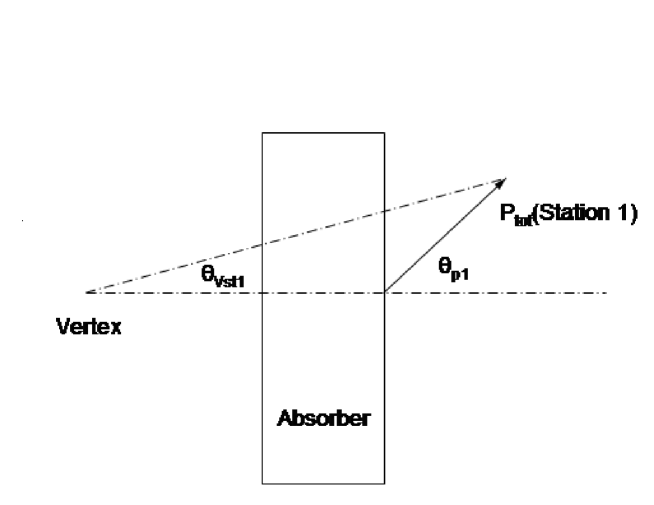
Figure 6.6: Sketch showing $\Delta\theta$ angular cut.

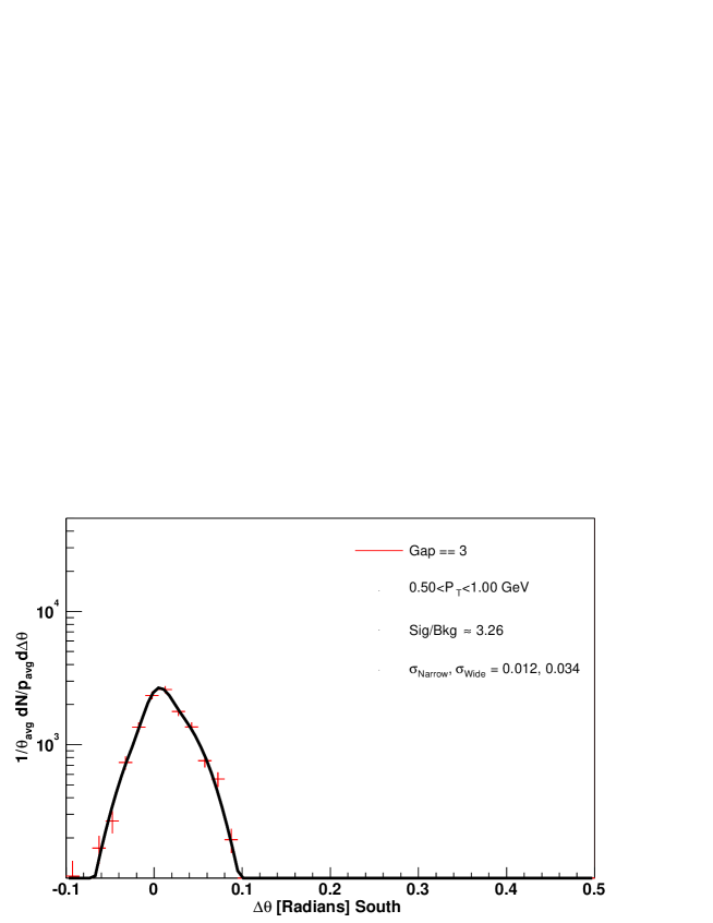
Figure 6.7: $\Delta\theta$ histogram for $0.5<p_{T}<1.0$ GeV/$c$, showing the wide peak of hadronic scattering and narrow peak of signal.

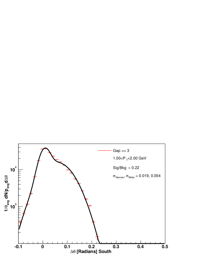
Figure 6.8: $\Delta\theta$ histogram for $1.0<p_{T}<2.0$ GeV/$c$.

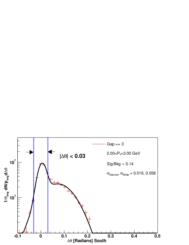
Figure 6.9: $\Delta\theta$ histogram for $2.0<p_{T}<3.0$ GeV/$c$, showing the wide peak of hadronic scattering and narrow peak of signal.

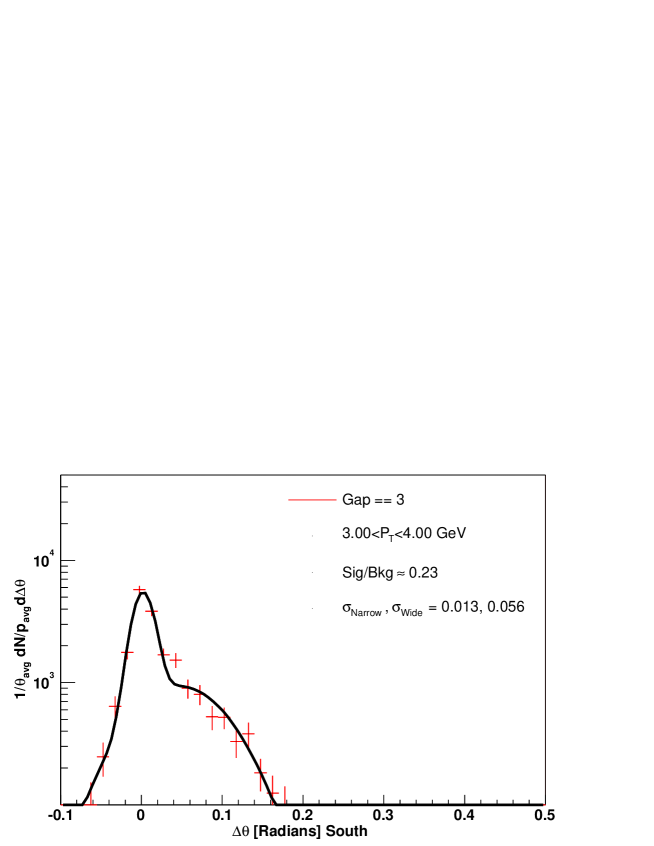
Figure 6.10: $\Delta\theta$ histogram for $3.0<p_{T}<4.0$ GeV/$c$.

For greater understanding we plot a 2D histogram of $\theta_{1}-\theta_{Vst1}$ vs $\theta_{Vst1}$ and $p_{tot}$ (see Fig. 6.11). We immediately see a large tail consistent with our expectation of showers. To cut this away without cutting too much signal, we apply a simple line cut $\Delta\theta<0.03$.

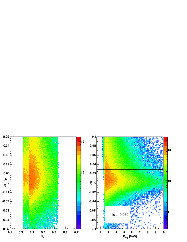
Figure 6.11: 2D histogram of $\theta_{1}-\theta_{Vecst1}$ vs $\theta_{1}$ and $p_{tot}$ ($0.5<p_{T}<3.5$ GeV) showing the cut.

6.4 Run QA

Runs used for this data analysis were selected after doing a Physics QA, by looking at several quantities like the average multiplicities. If the values were out of the average bands, the runs were rejected. This was done to reduce uncertainties from variation in detector acceptances due to tripped or dead channels, or beam background.

1. Beam Background: Due to the location of the muon arms, background due to beam can potentially be large. There are several cuts which can minimize this:

   1. It is expected that such a background will be coming from behind the muon arms and hence will hit the deepest MuID layers first. Since we are vetoing on the LASTGap (Gap 4), i.e., rejecting all tracks that make it to the LASTGap, this should considerably reduce this.

   2. If we look at the run-by-run variation in the number of hits (see Fig. 6.12), then beam background should lead to large fluctuations in this. And the variation in this number should give us an upper limit on the beam background.

   3. The $\Delta\theta$ angular cuts also reduce this because the angular distribution of the background is expected to be different from regular tracks.

2. MuID Efficiency: We are selecting hadrons by vetoing on the LASTGap (Gap 4). If the Gap 4 is switched off, or else if there is some sort of inefficiency in that panel, then all tracks would stop at Gap 3 instead of Gap 4, leading to a muonic contamination in our hadronic tracks. This contamination can be reduced by run QA. We looking at the run-by-run variation in the average value of the LASTGap (see Fig. 6.13). Any substantial inefficiency in Gap 4 (relative to our statistics), will lead to a drop in this value for that run.

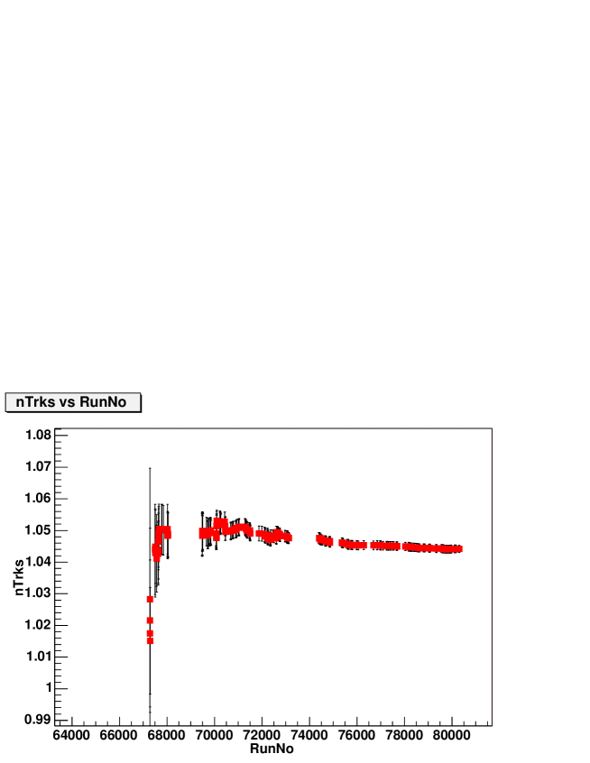
Figure 6.12: Run-by-run variation in npart.

Figure 6.13: Run-by-run variation in LASTGap.

Chapter 7 Hadron $R_{cp}$ measurement

We look at the particle multiplicities in forward and backward directions for d+Au collisions at $\sqrt{s_{NN}}=200$ GeV, and examine the behaviour as compared to mid-rapidity, as well their variation as a function of centrality. We can also compare results from d+Au collisions with those from Au+Au collisions in an attempt to distinguish between effects that could potentially be due to deconfinement, versus effects of cold nuclear matter.

7.1 $R_{cp}$ vs $p_{T}$

After obtaining the hadronic multiplicities as described in the previous chapter, we obtained the nuclear modification factor $R_{cp}$ by taking the ratios of multiplicities at a given centrality bin with the peripheral (60-92%) multiplicity scaled with the number of collisions $N_{coll}$, as defined previously in Eq. 5.1:

$$R_{cp}=\frac{\left(\frac{dN}{d\sigma dp_{T}}\right)^{Central}/N_{coll}^{Central}}{\left(\frac{dN}{d\sigma dp_{T}}\right)^{Peripheral}/N_{coll}^{Peripheral}}$$ (7.1)

We plotted $R_{cp}$ both as a function of transverse momentum $p_{T}$ and pseudorapidity $\eta$, for different centralities. The momentum fraction $x$ can be related to $p_{T}$ as: $x\approx p_{T}/\sqrt{s}$. Thus, greater the energy, lower is the value of $x$ we can get for a given $p_{T}$. It is important to stay at higher values of $p_{T}$ preferably $p_{T}>3$ GeV/$c$, so that we stay away from the soft regime, which is not very well described by standard perturbative QCD.

Figures 7.1,  7.2 and  7.3 show $R_{cp}$ vs $p_{T}$ for north and south arms for centralities 0-20%, 20-40% and 40-60% respectively (for data points see Table 7.1). We immediately notice:

1. $R_{cp}$ shows a suppression in the North Arm (d going direction) and an enhancement in the South Arm (Au going direction).

2. The suppression is maximum for 0-20% centrality and decreases for less central collisions. The enhancement too is maximum for 0-20% centrality and decreases for less central collisions.

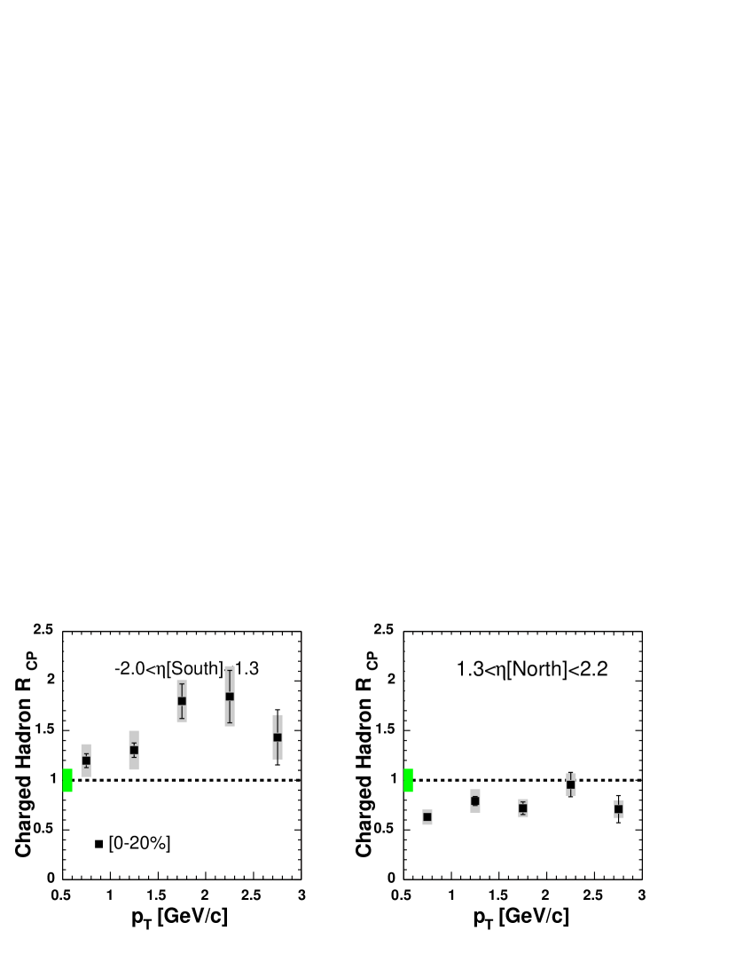
Figure 7.1: $R_{cp}$ vs $p_{T}$ for all charged hadrons for 0-20% most central events. Left panel shows data from the South Arm ($-2.2<\eta<-1.2$), while the right panel shows data from North Arm($1.2<\eta<2.4$). Systematic errors that vary point by point are shown by grey bars at each data point, while errors are same for all points are depicted by the green bar. (PHENIX Preliminary)

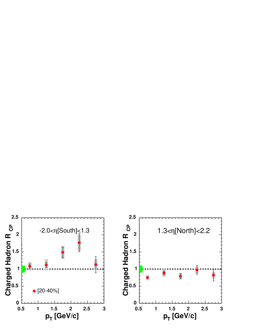
Figure 7.2: $R_{cp}$ vs $p_{T}$ for all charged hadrons for 20-40% most central events. Left panel shows data from the South Arm ($-2.2<\eta<-1.2$), while the right panel shows data from North Arm($1.2<\eta<2.4$). Systematic errors that vary point by point are shown by grey bars at each data point, while errors are same for all points are depicted by the green bar.(PHENIX Preliminary)

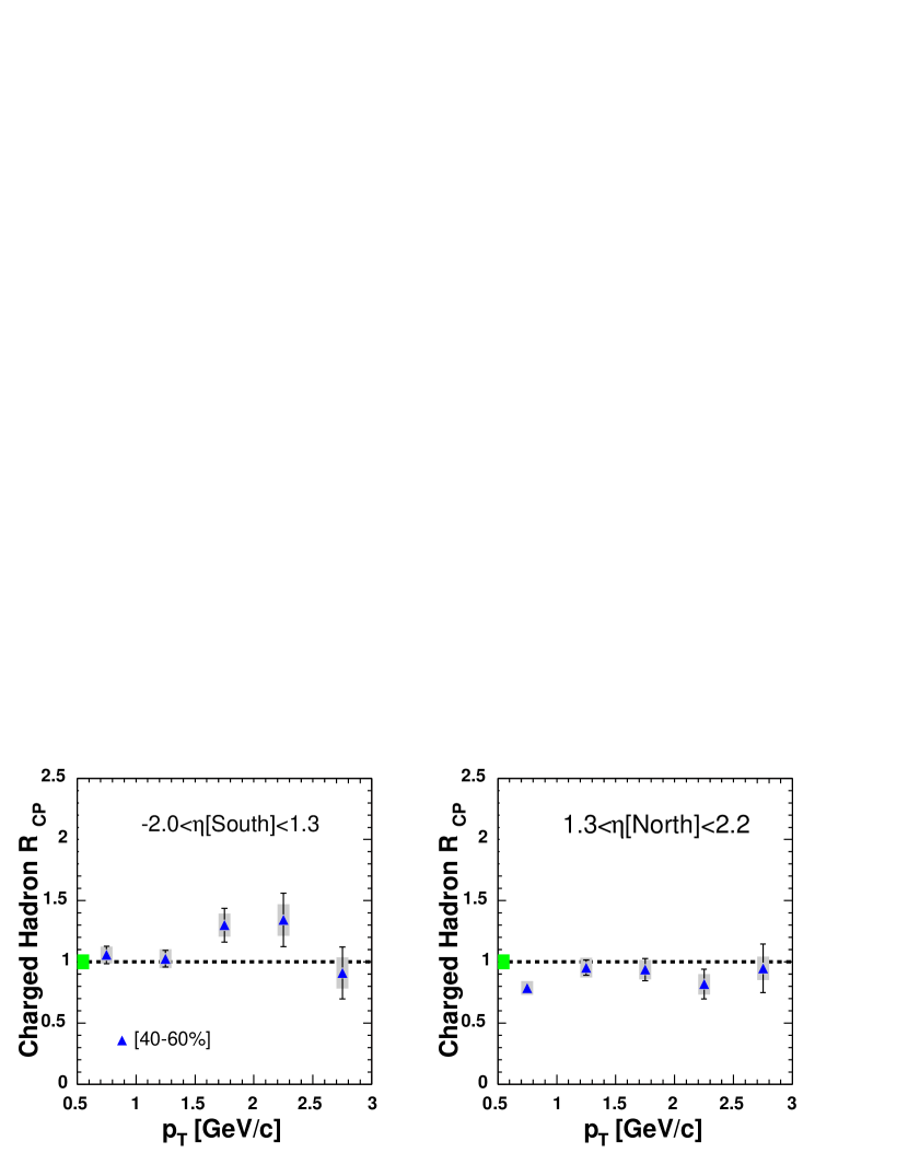
Figure 7.3: $R_{cp}$ vs $p_{T}$ for all charged hadrons GeV for 40-60% most central events. Left panel shows data from the South Arm ($-2.2<\eta<-1.2$), while the right panel shows data from North Arm($1.2<\eta<2.4$). Systematic errors that vary point by point are shown by grey bars at each data point, while errors are same for all points are depicted by the green bar.(PHENIX Preliminary)

We classify our systematic uncertainties for $R_{cp}$ vs $p_{T}$ measurement in two categories:

1. Those which vary point to point for each data point in $p_{T}$ (listed in Tables 7.2 and  7.3 for the South and North Arms respectively):

   1. Potential shower contamination: this was determined by varying the polar angle $\Delta\theta$ cut from 0.03 to 0.06.

   2. Potential beam background: this can be estimated by varying the acceptance cut from $15^{o}$ to $12^{o}$.

2. Those which are constant for each data point(listed in Table 7.4):

   1. Uncertainty on number of binary collisions $N_{coll}$: $10.8\%$ [23] for 0-20% centrality. It varies as a function of centrality.

   2. Tracking/road finding efficiency:$\approx 4\%$. This primarily occurs because the track reconstruction system in the muon arms can misidentify tracks.

Table 7.1: Data table for $R_{cp}$ vs $p_{T}$ for North and South Arms. All errors are statistical. Systematic uncertainties are given in Tables 7.2, 7.3 and 7.4.

Centrality	$p_{T}$ [GeV/$c$]	$R_{cp}$(South)	$R_{cp}$(North)
	0.5 - 1.0	1.19735$\pm$0.0706	0.629646$\pm$0.0321
	1.0 - 1.5	1.30357$\pm$0.0743	0.790778$\pm$0.0467
0-20%	1.5 - 2.0	1.79743$\pm$0.1744	0.718265$\pm$0.0639
	2.0 - 2.5	1.84448$\pm$0.2638	0.955506$\pm$0.1223
	2.5 - 3.0	1.43172$\pm$0.2778	0.708701$\pm$0.1361
	0.5 - 1.0	1.08141$\pm$0.0681	0.751891$\pm$0.0399
	1.0 - 1.5	1.12044$\pm$0.0683	0.888502$\pm$0.0551
20-40%	1.5 - 2.0	1.48803$\pm$0.1458	0.789919$\pm$0.0735
	2.0 - 2.5	1.77024$\pm$0.262	0.974458$\pm$0.1306
	2.5 - 3.0	1.13006$\pm$0.2351	0.823329$\pm$0.1647
	0.5 - 1.0	1.05717$\pm$0.0719	0.785904$\pm$0.0448
	1.0 - 1.5	1.0257 $\pm$0.0677	0.95276$\pm$0.0629
40-60%	1.5 - 2.0	1.29969$\pm$0.1378	0.936201$\pm$0.0908
	2.0 - 2.5	1.3429 $\pm$0.2175	0.817881$\pm$0.1227
	2.5 - 3.0	0.909452$\pm$0.2119	0.946805$\pm$0.1979

Table 7.2: Point to point systematic uncertainties for $R_{cp}$ in South Arm.

Centrality	$p_{T}$[GeV/$c$]	$\Delta\theta$ cut	Acceptance	Total $p_{T}$ dependent systematics
	0.5-1.0	2.90%	6.80%	7.39%
	1.0-1.5	5.70%	7.40%	9.34%
0-20%	1.5-2.0	1.10%	2.40%	2.64%
	2.0-2.5	8.00%	8.30%	11.53%
	2.5-3.0	9.30%	5.10%	10.61%
	0.5-1.0	1.50%	5.10%	5.32%
	1.0-1.5	8.40%	6.30%	10.50%
20-40%	1.5-2.0	7.30%	4.40%	8.52%
	2.0-2.5	1.30%	8.20%	8.30%
	2.5-3.0	9.50%	0%	9.50%
	0.5-1.0	1.80%	0.50%	1.87%
	1.0-1.5	3.20%	3.00%	4.39%
40-60%	1.5-2.0	3.20%	1.70%	3.62%
	2.0-2.5	2.80%	6.70%	7.26%
	2.5-3.0	11.30%	5.30%	12.48%

Table 7.3: $p_{T}$ systematic uncertainties for $R_{cp}$ in North Arm.

Centrality	$p_{T}$[GeV/$c$]	$\Delta\theta$ cut	Acceptance	Total $p_{T}$ dependent systematics
	0.5-1.0	2.80%	1.90%	3.38%
	1.0-1.5	6.80%	6.90%	9.69%
0-20%	1.5-2.0	2.20%	4.30%	4.83%
	2.0-2.5	0.30%	3.10%	3.11%
	2.5-3.0	1.30%	4.30%	4.49%
	0.5-1.0	0.50%	1.40%	1.49%
	1.0-1.5	4.10%	5.80%	7.10%
20-40%	1.5-2.0	5.50%	2.90%	6.22%
	2.0-2.5	1.50%	1.10%	1.86%
	2.5-3.0	3.80%	5.00%	6.28%
	0.5-1.0	2.50%	2.60%	3.61%
	1.0-1.5	2.80%	4.90%	5.64%
40-60%	1.5-2.0	4.30%	3.50%	5.54%
	2.0-2.5	8.00%	0.40%	8.01%
	2.5-3.0	5.20%	6.00%	7.94%

Table 7.4: $p_{T}$ independent systematics for $R_{cp}$.

Centrality	$n_{binary}$	Tracking/roadfinding
0-20%	10.80%	4%
20-40%	9.30%	4%
40-60%	4.80%	4%

7.2 $R_{cp}$ vs $\eta$

Using the same methodology described above, we calculated $R_{cp}$ vs $\eta$ by integrating our data in the range $1<p_{t}<3$ GeV/$c$, for each $\eta$ bin. The $\eta$ range goes from -2.2 to -1.2 for the South Arm to 1.2 to 2.4 for the North Arm. In addition there is also a data point at midrapidity using previous results from the PHENIX Central Arm [23]. Figures 7.4,  7.5 and  7.6 show plots of $R_{cp}$ vs $\eta$ for the centrality ranges 0-20%, 20-40% and 40-60% respectively (for data points see Table 7.5). We notice two main trends:

1. $R_{cp}$ shows a suppression in the North Arm (d going direction) and an enhancement in the South Arm (Au going direction) and this increase is continuous and almost linear as we go from $\eta=-2.2$ in the South Arm to $\eta=2.4$ in the North Arm.

2. The suppression (and enhancement) is maximum for 0-20% centrality and decreases for less central collisions.

Table 7.5: $R_{cp}$ vs $\eta$ in the range $1<p_{t}<3$ GeV/$c$.

Centrality	$\eta$	$R_{cp}$
	-1.88333	1.76019 $\pm$ 0.13991
	-1.65	1.64172 $\pm$ 0.0631918
	-1.41667	1.53932 $\pm$ 0.0892065
0-20%	1.4125	1.00895 $\pm$ 0.0741331
	1.6375	0.922162 $\pm$ 0.0442295
	1.8625	0.795191 $\pm$ 0.0279444
	2.0875	0.781327 $\pm$ 0.0771171
	-1.88333	1.40951 $\pm$ 0.119334
	-1.65	1.40715 $\pm$ 0.0573594
	-1.41667	1.36865 $\pm$ 0.0838189
20-40%	1.4125	0.965126 $\pm$ 0.0754662
	1.6375	0.937888 $\pm$ 0.0475359
	1.8625	0.8784 $\pm$ 0.0323008
	2.0875	0.890123 $\pm$ 0.0914602
	-1.88333	1.26621 $\pm$ 0.115834
	-1.65	1.21456 $\pm$ 0.0539039
	-1.41667	1.15746 $\pm$ 0.0776094
40-60%	1.4125	1.09681 $\pm$ 0.0899434
	1.6375	0.953508 $\pm$ 0.0519437
	1.8625	0.919708 $\pm$ 0.0362131
	2.0875	0.962761 $\pm$ 0.105112

Systematics for $R_{cp}$ vs $\eta$ are again of two types:

1. Point-to-point systematic uncertainties, which vary from one data point to another (see Table 7.6):

   1. Systematic uncertainty in the $p_{tot}$ cut (which is used to reject muons stopped in the shallow MuID Gaps) is calculated by varying our $p_{tot}$ cut by $1\sigma$ from 1.9 GeV to 2.1 GeV.

   2. Systematic uncertainty in $p_{T}$ is calculated by varying our $p_{T}$ range from 1.0—2.0 GeV, to 1.2—2.2 GeV.

   3. Since we integrate over a given $p_{T}$ range for each $\eta$ bin, we need to determine the systematic uncertainty due to $p_{T}$. This is calculated by varying our $p_{T}$ range from 1.0–3.0 GeV, to 1.2–3.2 GeV.

   4. Systematic uncertainty in $\Delta\theta$ cut (which is used to reject hadronic showers) is calculated by varying it from $\Delta\theta<0.030$ to $\Delta\theta<0.060$.

2. Then there are systematic uncertainties that are independent of $\eta$. These consist of uncertainty in $N_{coll}$, the number of collisions in a given centrality bin and tracking/roadfinding efficiency. These were tabulated earlier in Table 7.4.

Table 7.6: Point-to-point systematics for $R_{cp}$ vs $\eta$ in the range $1<p_{t}<3$ GeV/$c$.

Centrality	$\eta$	$p_{tot}$	$p_{T}$	$\Delta\theta$	Total point-to-point systematics
	-1.88333	0.42%	7%	4.36%	8.26%
	-1.65	1.11%	1.1%	0.86%	1.78%
	-1.41667	0.47%	8.52%	0.88%	8.58%
0-20%	1.4125	2.48%	0.63%	0.41%	2.59%
	1.6375	2.57%	3.57%	1.65%	4.70%
	1.8625	0.08%	5.06	1.94%	5.42%
	2.0875	0%	4.7%	0.55%	4.73%
	-1.88333	0.1%	1.44%	0.56%	1.55%
	-1.65	1.32%	1.83%	0.48%	2.31%
	-1.41667	0.37%	2.95%	0.41%	3.00%
20-40%	1.4125	1.12%	2.84%	0.98%	3.21%
	1.6375	2.62%	0.56%	0.44%	2.72%
	1.8625	0.14%	3.56%	1.48%	3.86%
	2.0875	0%	3.08%	1.76%	3.55%
	-1.88333	0.19%	3.82%	5.35%	6.58%
	-1.65	1.3%	1.93%	1.23%	2.63%
	-1.41667	2.97%	2.63%	0.09%	3.97%
40-60%	1.4125	3.15%	1.53%	0.07%	3.50%
	1.6375	2.2%	4.16%	0.49%	4.73%
	1.8625	0.07%	2.65%	2.64%	3.74%
	2.0875	0%	3.44%	5.44%	6.44%

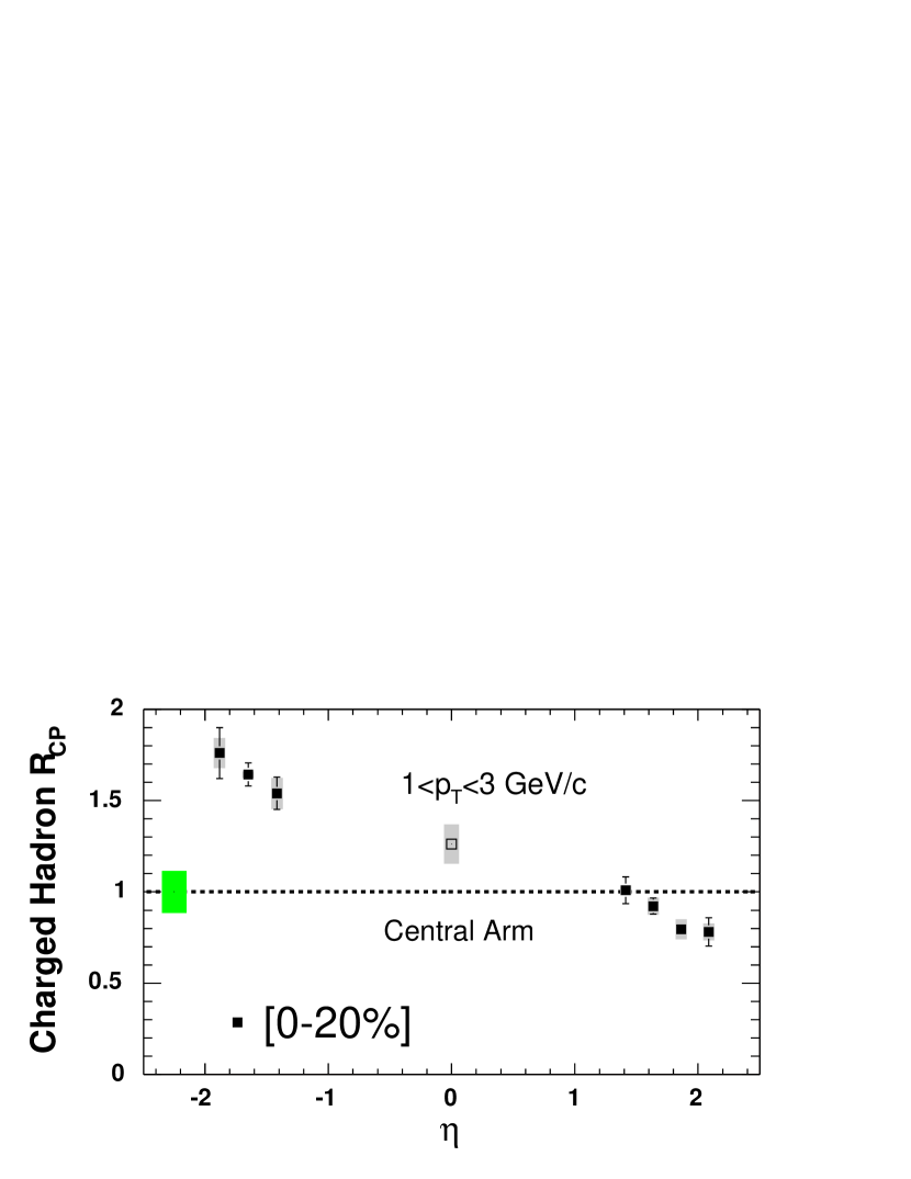
Figure 7.4: $R_{cp}$ vs $\eta$ for all charged hadrons in the range $1<p_{t}<3$ GeV/$c$ for 0-20% most central events. Au going direction is along negative $\eta$ (South Arm) and d going direction is along positive $\eta$ (North Arm). Systematic errors that vary point by point are shown by grey bars at each data point, while errors are same for all points are depicted by the green bar.(PHENIX Preliminary)

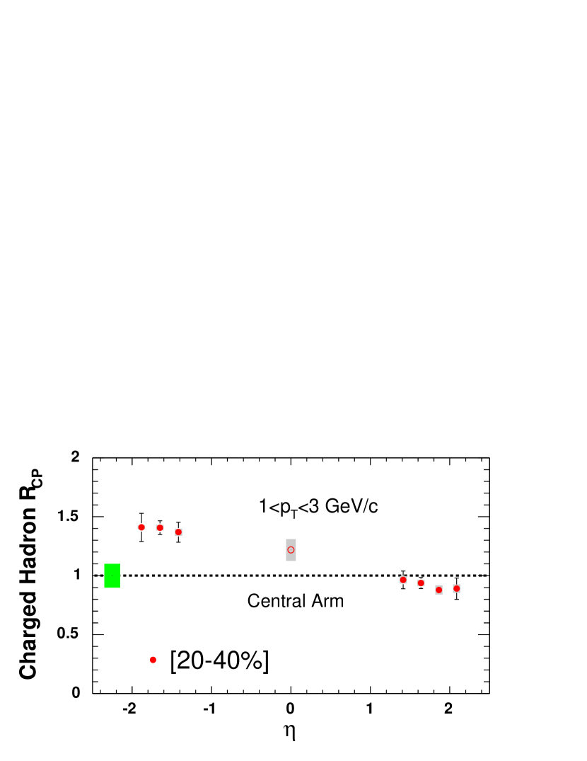
Figure 7.5: $R_{cp}$ vs $\eta$ for all charged hadrons in the range $1<p_{t}<3$ GeV/$c$ for 20-40% most central events. Au going direction is along negative $\eta$ (South Arm) and d going direction is along positive $\eta$ (North Arm). Systematic errors that vary point by point are shown by grey bars at each data point, while errors are same for all points are depicted by the green bar.(PHENIX Preliminary)

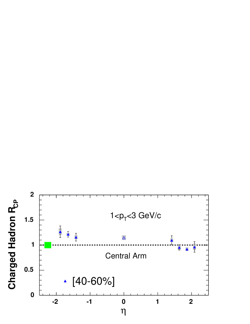
Figure 7.6: $R_{cp}$ vs $\eta$ for all charged hadrons in the range $1<p_{t}<3$ GeV/$c$ for 40-60% most central events. Au going direction is along negative $\eta$ (South Arm) and d going direction is along positive $\eta$ (North Arm). Systematic errors that vary point by point are shown by grey bars at each data point, while errors are same for all points are depicted by the green bar.(PHENIX Preliminary)

The plots shown earlier in Figures 7.4, 7.5, 7.6, 7.1, 7.2, 7.3 were for minimum bias data only. In order to improve statistics and increase the momentum range, triggered data was used to obtain better plots [61], which can be seen in Figures 7.7 and 7.8. Special thanks goes to Chun Zhang and Ming X. Liu for Figures 7.7 and 7.8.

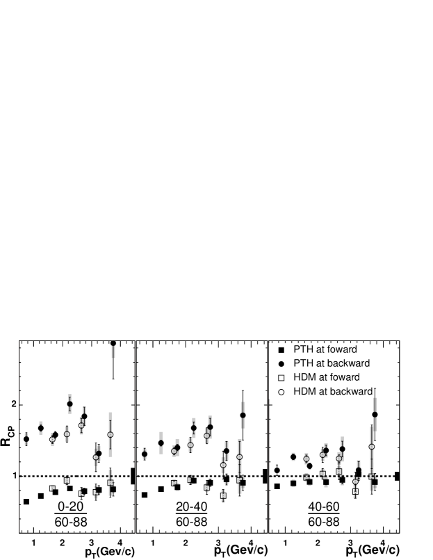
Figure 7.7: $R_{cp}$ vs $p_{T}$ for triggered data. PTH stands for punch through hadrons, whereas HDM stands for data from hadron decay mesons.

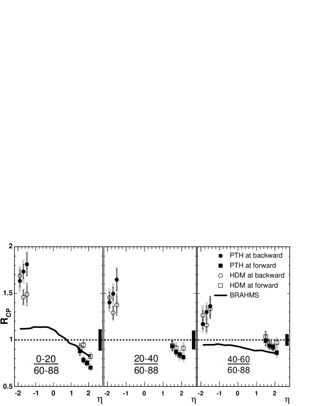
Figure 7.8: $R_{cp}$ vs $\eta$ for triggered data. PTH stands for punch through hadrons, whereas HDM stands for data from hadron decay mesons. The solid line depicts a fit to the BRAHMS data [62] for comparison. (PHENIX Preliminary Data)

7.3 Comparisons

Our data on hadron $R_{cp}$ indicates a suppression on the forward region (d going direction). Similar behaviour was also seen by BRAHMS experiment REFS? at RHIC. This is qualitatively consistent with shadowing/saturation type effects in the small-$x$ region being probed at forward rapidities. Moreover, the central to peripheral $R_{cp}$ (Figure 7.4) is more suppressed as compared to semi-central to peripheral $R_{cp}$ (Figure 7.5).

As mentioned previously (Chapter 5), the Color Glass Condensate model gives a universal QCD explanation for low-$x$ shadowing and predicts a depletion in scattering centers due to gluon processes. The small-$x$ regions can be probed by going to forward rapidities (see Eq.5.2). A toy model prediction [25] is made regarding variation of $R_{cp}$ as a function of rapidity. In Figure 7.9 $R^{pA}$ (which is equivalent to $R_{cp}$ if we assume that peripheral collisions are analogous to p+p collisions) is plotted vs $k/Q_{s}$, where $k$ is the transverse momentum of the partons and $Q_{s}$ is the saturation scale, given by:

$$Q_{s}(y)\approx Q_{s0}e^{2\bar{\alpha}y}$$ (7.2)

As the rapidity (or equivalently energy) increases, the upper solid curve slowly turns into the lower solid curve. It is also predicted that as the collision centrality increases $R^{pA}$ will decrease, consistent with our observations.

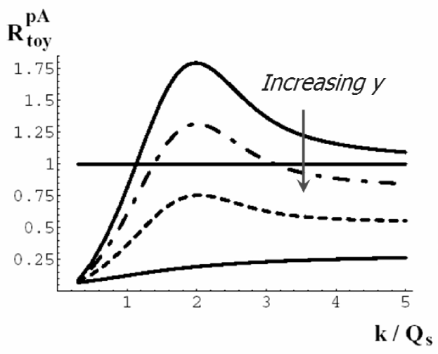
Figure 7.9: $R^{pA}$ vs $k/Q_{s}$ as predicted by CGC model [25]. The nuclear modification factor decreases with rapidity.

On the other hand, the backward rapidity region (Au going direction) is very different. We see an enhancement, which is not satisfactorily explained by the CGC model, which predicts a flat distribution in the backward region. This sort of enhancement has been seen at other experiments and is known as the Cronin effect, and is usually attributed to initial multiple scatterings at the partonic level. Another candidate is anti-shadowing, which occurs when $g+g\rightarrow g$ processes deplete partons at small-$x$ partons but increase those at larger-$x$ (and momenta). Although, we should note that our momentum range of 1–3 GeV/$c$ is not completely in the hard scattering regime. Hence we factorisation might not apply and we might be sensitive to soft physics. In such a scenario, the backward enhancement could be explained by rapidity exchange. Early studies [63] have shown that in a p+Pb collision with p incident at 100 GeV/$c$ on Pb at rest, the rapidity exchange $\simeq$ 2.5. However RHIC is at a much higher energy and so this rapidity exchange is expected to a small effect. Thus, at present, there is no single satisfactory explaination for the enhancement in the backward direction.

In addition we can also include results from the PHENIX $J/\psi$ measurements for comparison. It is interesting to look at the $J/\psi$ because due to its heavy mass, it is mostly produced by gluon gluon fusion processes (see Figure 7.10). Hence $J/\psi$ production is an independent probe of gluon PDFs. In Figure 7.11 we plot hadrons from PHENIX and BRAHMS (in a different $\eta$ range) as well as the $J/\psi$ from PHENIX, we notice that that $R_{cp}$ (vs $\eta$) is almost a straight line.

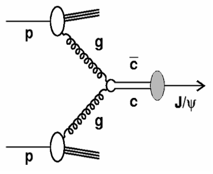
Figure 7.10: Due to its heavy mass, at RHIC energies $J/\psi$ is produced mostly via $g+g\rightarrow J/\psi$.

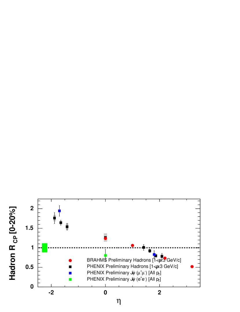
Figure 7.11: Comparison of PHENIX Preliminary hadron $R_{cp}$ with that of BRAHMS, and PHENIX $J/\psi$.

There is no simple explanation why all this data falls in a straight line. The $J/\psi$ results are especially puzzling because of the differing production mechanisms. Other models like the recombination model [64] make only make some qualitative predictions regarding the $\eta$ dependence.

Chapter 8 Summary

We studied the final state effects of the produced matter from ultrarelativistic Au+Au collisions at $\sqrt{s_{NN}}=200$ GeV, by looking at the production of the simplest nuclei: deuterons and anti-deuterons. The transverse momentum spectra of $d$ and $\bar{d}$ in the range $1.1<p_{T}<4.3$ GeV/$c$ were measured at mid-rapidity and were found to be less steeply falling than proton (and antiproton) spectra. This seems to be consistent with a constant (flat) source density profile. The extracted coalescence parameter $B_{2}$ increases with $p_{T}$, which is indicative of an expanding source. $B_{2}$ decreases for more central collisions, consistent with an increasing source size with centrality. The $B_{2}$ measured in nucleus-nucleus collisions is independent of $\sqrt{s_{NN}}$ above 12 GeV, consistent with Bose-Einstein correlation measurements of the radii of the source. $B_{2}$ is equal within errors for both deuterons and anti-deuterons. From the measurements, it is estimated that $\bar{n}/n$ = 0.64 $\pm$ 0.04.

We studied the effect of cold nuclear matter in d+Au collisions at $\sqrt{s_{NN}}=200$ GeV, by looking at particle production in forward and backward directions. $R_{cp}$ was observed to be suppressed at Au+Au collisions at $\sqrt{s_{NN}}=200$ GeV [19, 20, 21, 22], at mid-rapidity. This was consistent either with prediction of jet suppression due to energy loss in the dense partonic matter created in Au+Au collisions  [58, 59] or with the depletion of low-$x$ partons due to gluon saturation or Color-Glass Condensate (CGC) hypothesis [25, 26, 27]. When the d+Au control experiment was done to verify whether or not the suppression seen in Au+Au was due to final state effects (jet suppression) or due to initial state effects (changes in the parton distribution functions) an enhancement was seen for $R_{cp}$ at mid-rapidity [23, 24]. This means that CGC does not describe the mid-rapidity distributions and not is applicable in that regime. There is a different story at forward rapidity, where the position of the Muon Arms enables us to probe small values of the momentum fraction $x$. We found hadron $R_{cp}$ to be suppressed at forward rapidities (d going direction). This is qualitatively consistent with shadowing/saturation type effects in the small-$x$ region being probed at forward rapidities. $R_{cp}$ was enhanced at backward rapidities (Au going region). If we include other data: the PHENIX $J/\psi$ and charged hadron $R_{cp}$ from BRAHMS, and plot $R_{cp}$ vs $\eta$, we found that the data almost lies on a straight line. Although the suppression at forward rapidites can be qualitatively understood using the CGC model, however the enhancement at backward rapidities remains a mystery. Although, we should note that our momentum range of 1–3 GeV/$c$ is not completely in the hard scattering regime. Hence factorisation might not apply and we might be sensitive to soft physics. In such a scenario, the backward enhancement could be explained by rapidity exchange. Early studies [63] have shown that in a p+Pb collision with p incident at 100 GeV/$c$ on Pb at rest, the rapidity exchange $\simeq$ 2.5. However RHIC is at a much higher energy and so this rapidity exchange is expected to a small effect. Thus, at present, there is no single satisfactory explaination for the enhancement in the backward direction.

In the near future, we plan to try to measure $R_{cp}$ for the prompt muons, i.e., muons produced at the vertex mostly from charm decays. This could give us some insight on flavor dependence of saturation effects in d+Au collisions. For Au+Au, this could give us insight on jet suppression mechanisms, for instance gluon bremstrahlung type radiative suppression will depend on the mass of the quark, and be lesser for charm and other heavy quarks. Another measurement would be doing d+Au collisions at an intermediate energy between AGS and current RHIC energies to fill in the gaps in previous experiments. Further in the future, exciting new measurements can be made using the proposed electron beam accelerator eRHIC at BNL, which will be capable of e+A (and polarized protons). Color Glass Condensate model makes very different predictions for the gluon PDFS as compared to conventional pQCD calculations. eRHIC can help us to gain insight into the small-$x$ behaviour of gluons. Another interesting study would be the parton propagation through nuclei, which can lead to $p_{T}$ broadening and help us gain a better understanding of the Cronin effect.

Appendix A Comparison between Data and Monte Carlo

In order to ensure that our matching cuts (or track residuals): $\sigma_{\phi}(TOF,PC3)$ and $\sigma_{z}(TOF,PC3)$ are well matched between data and MC, we have plotted them against variables like $z$, centrality, $p_{T}$ and so on, for first for the data and then for the Monte Carlo (MC).

A.1 Matching systematics for data

Figure A.1: $\sigma_{\phi}(TOF)$ matching variable vs $z$ for data.

Figure A.2: $\sigma_{\phi}(TOF)$ matching variable vs $p_{T}$ for data.

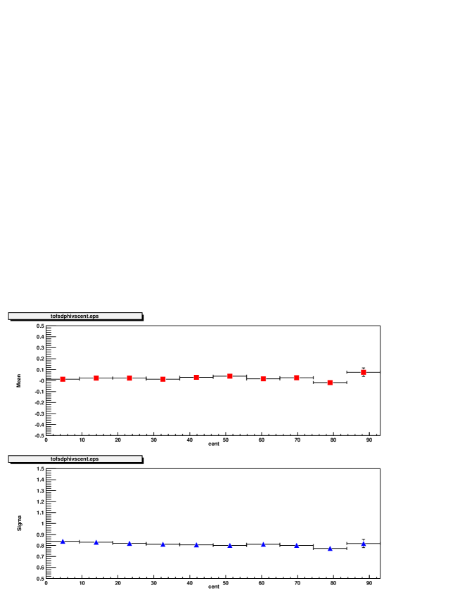
Figure A.3: $\sigma_{\phi}(TOF)$ matching variable vs Centrality for data.

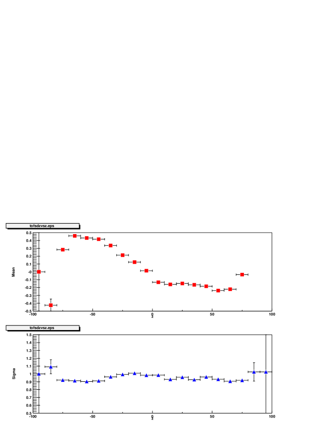
Figure A.4: $\sigma_{z}(TOF)$ matching variable vs $z$ (as measured in DC) for data.

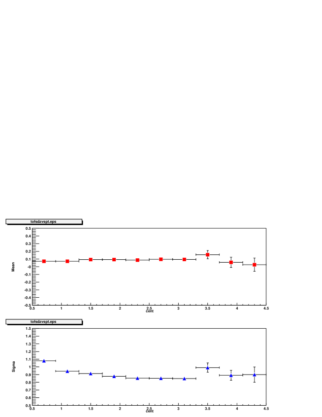
Figure A.5: $\sigma_{z}(TOF)$ matching variable vs $p_{T}$ for data.

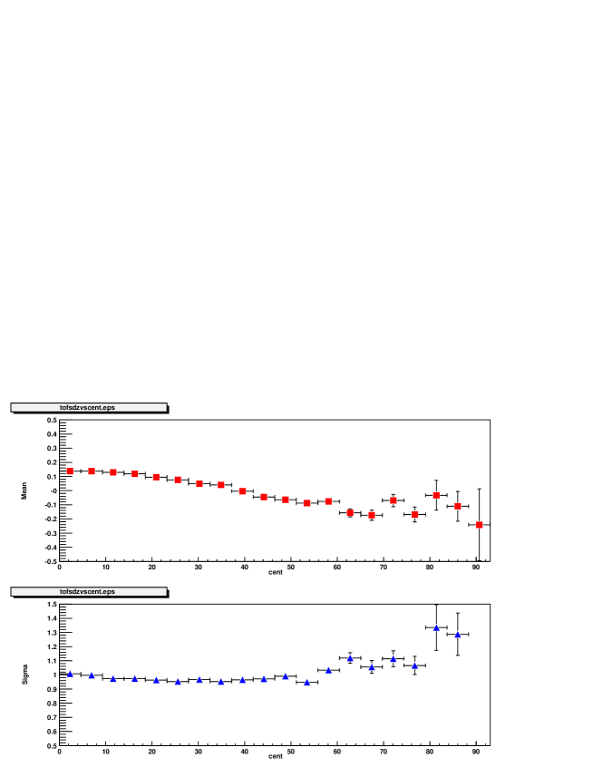
Figure A.6: $\sigma_{z}(TOF)$ matching variable vs Centrality for data.

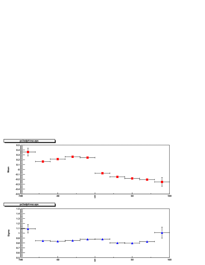
Figure A.7: $\sigma_{\phi}(PC3)$ matching variable vs $z$ (as measured in DC) for data.

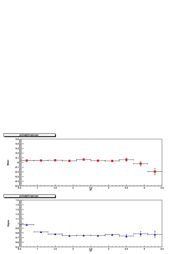
Figure A.8: $\sigma_{\phi}(PC3)$ matching variable vs $p_{T}$ for data.

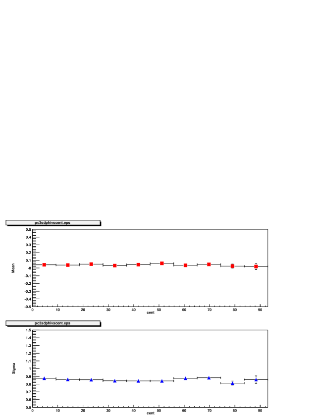
Figure A.9: $\sigma_{\phi}(PC3)$ matching variable vs centrality for data.

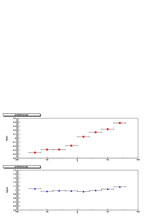
Figure A.10: $\sigma_{z}(PC3)$ matching variable vs $z$ for data.

Figure A.11: $\sigma_{z}(PC3)$ matching variable vs $p_{T}$ for data.

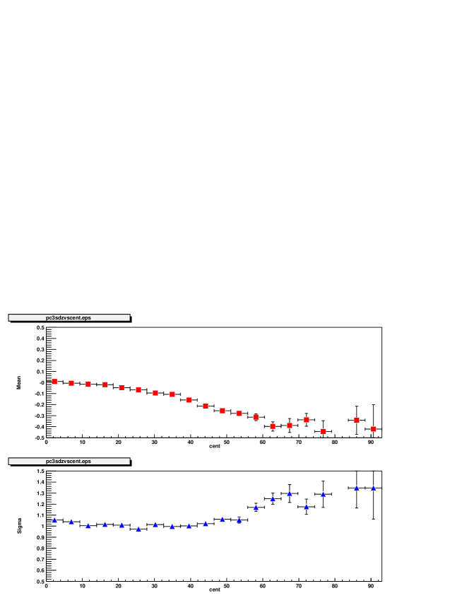
Figure A.12: $\sigma_{z}(PC3)$ matching variable vs centrality for data.

A.2 Matching systematics in MC

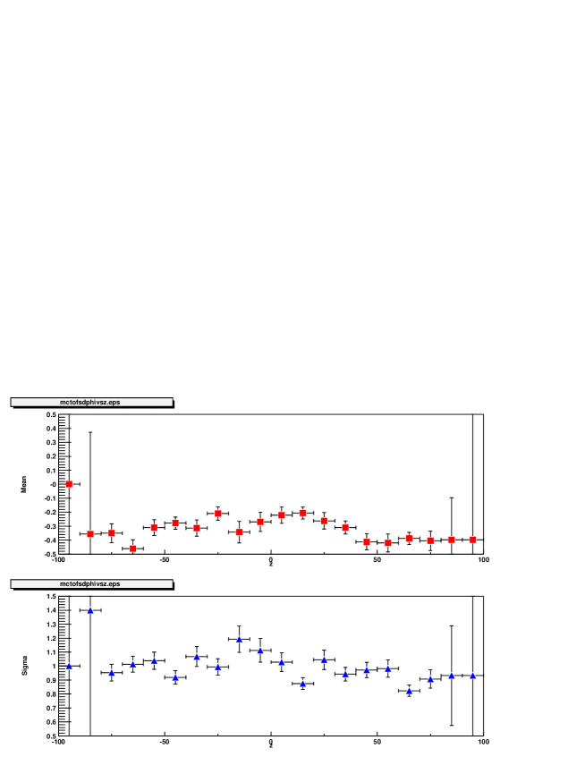
Figure A.13: $\sigma_{\phi}(TOF)$ matching variable vs $z$ in MC

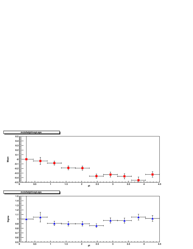
Figure A.14: $\sigma_{\phi}(TOF)$ matching variable vs $p_{T}$ in MC

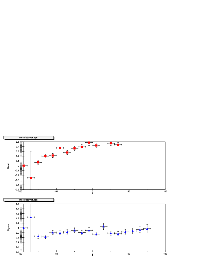
Figure A.15: $\sigma_{z}(TOF)$ matching variable vs $z$ in MC

Figure A.16: $\sigma_{z}(TOF)$ matching variable vs $p_{T}$ in MC

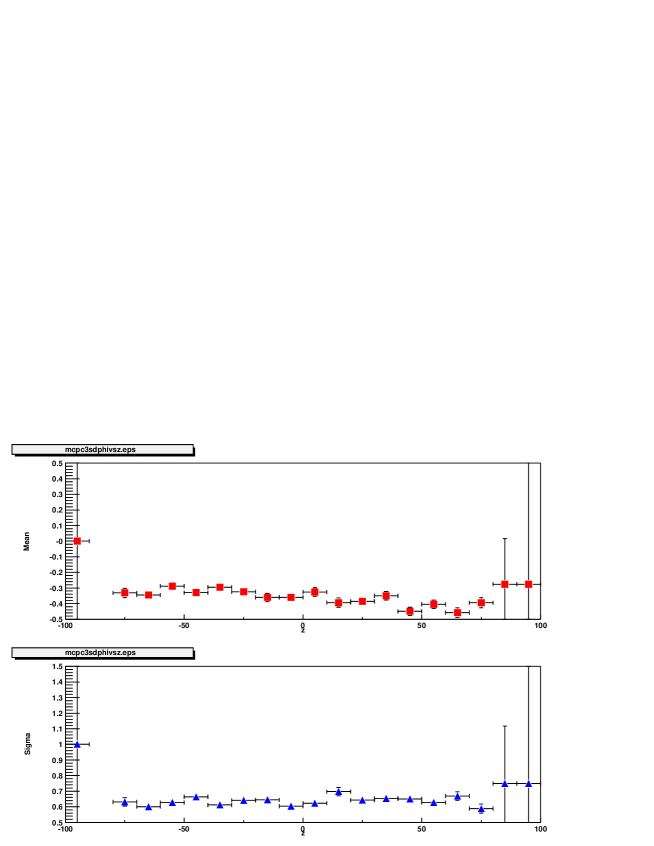
Figure A.17: $\sigma_{\phi}(PC3)$ matching variable vs $z$ in MC

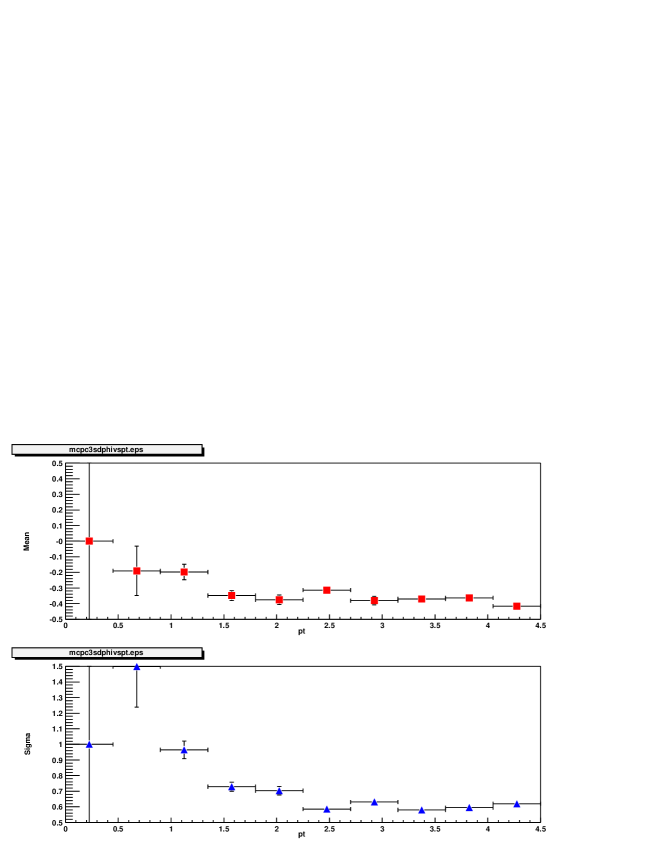
Figure A.18: $\sigma_{\phi}(PC3)$ matching variable vs $p_{T}$ in MC

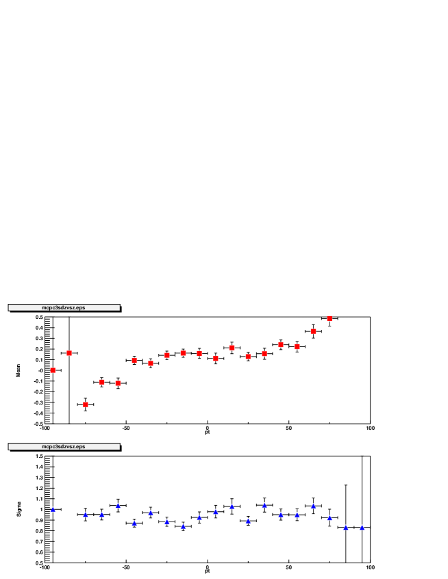
Figure A.19: $\sigma_{z}(PC3)$ matching variable vs $z$ in MC

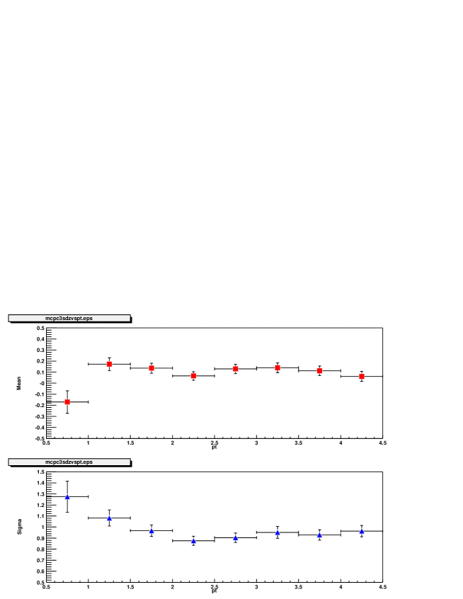
Figure A.20: $\sigma_{z}(PC3)$ matching variable vs $p_{T}$ in MC

A.3 Comparison of acceptance between data and MC

We also need to check that our MC simulations match each detector’s characteristics as accurately as possible. To cross check this, we look at track and hit distributions for acceptance both in MC and data.

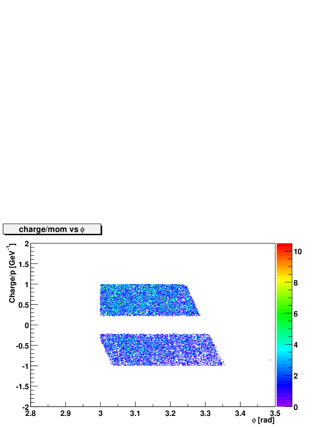
Figure A.21: Charge/$p$ vs Dch $\phi$ in data.

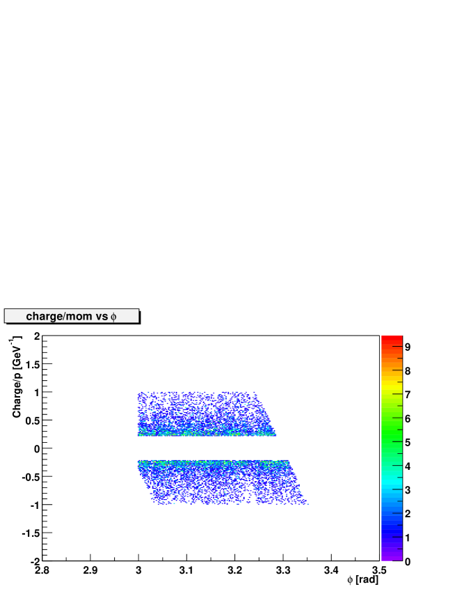
Figure A.22: Charge/$p$ vs DC $\phi$ in MC.

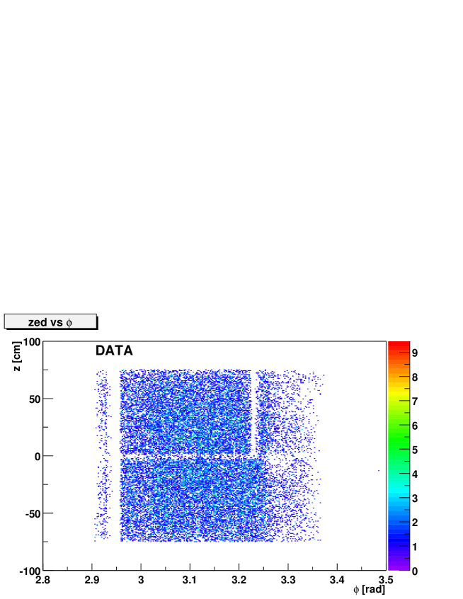
Figure A.23: $z$ vs DC $\phi$ in data.

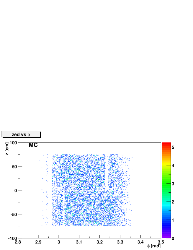
Figure A.24: $z$ vs DC $\phi$ in MC.

Bibliography

- [1] J. D. Bjorken, Phys. Rev. D27, 140 (1983)
- [2] For a review see: F. Karsch, Nucl. Phys. A698, 199c (2002)
- [3] A long range plan for nuclear science, DOE/NSF, Dec. 1983
- [4] For a review of dilepton production see: P. V. Ruuskanen, Nucl. Phys. A522, 255c (1991) and P. V. Ruuskanen, Nucl. Phys. A544, 169c (1992).
- [5] For a review of photon production see: J. Kapusta, P. Lichard and D. Siebert, Nucl. Phys. A544, 485c (1992) and P. V. Ruuskanen, Nucl. Phys. A544, 169c (1992).
- [6] J. Rafelski Nucl. Phys. A544, 279c (1992); H. C. Eggers and J. Rafelski, Int. J. Mod. Phys. A6, 1067 (1991); P. Koch, B. Müller and J. Rafelski, Phys. Rep. 142, 167 (1986).
- [7] T. Matsui and H. Satz, Phys. Lett. B178, 416 (1986); T. Matsui, Z. Phys. C38, 245 (1988).
- [8] R. Hanbury-Brown and R. Q. Twiss, Phil. Mag. 45, 633 (1954).
- [9] M. Gyulassy and M. Plümer, Phys. Lett. B243, 432 (1990); X. N. Wang and M. Gyulassy, Phys. Rev. Lett. 68, 1480 (1992); R. Baier et al, Phys. Lett. B345, 277 (1995);
- [10] K. Adcox et al. [PHENIX Collaboration], Phys. Rev. Lett. 86, 3500 (2001).
- [11] B. B. Back et al. [PHOBOS Collaboration], Phys. Rev. Lett. 88, 022302 (2002).
- [12] K. Adcox et al. [PHENIX Collaboration], Phys. Rev. Lett. 88, 242301 (2002).
- [13] B. B. Back et al. [PHOBOS Collaboration], Phys. Rev. C67, 021901 (2003).
- [14] C. Adler et al. [STAR Collaboration], Phys. Rev. Lett. 86, 4778 (2001).
- [15] L. P. Csernai and J. I. Kapusta, Phys. Rep. 131, 223 (1986).
- [16] A. Z. Mekjian, Phys. Rev. C17, 1051 (1978).
- [17] K. Adcox et al. [PHENIX Collaboration], Phys. Rev. C69, 024904 (2004).
- [18] S. S. Adler et al. [PHENIX Collaboration], nucl-ex/0307022.
- [19] K. Adcox et al. [PHENIX Collaboration], Phys. Rev. Lett. 88, 022301 (2002).
- [20] K. Adcox et al. [PHENIX Collaboration], Phys. Lett. B561, 82 (2003).
- [21] C. Adler et al. [STAR Collaboration], Phys. Rev. Lett. 89, 202301 (2002).
- [22] S. S. Adler et al. [PHENIX Collaboration], Phys. Rev. Lett. 91, 241803 (2002).
- [23] S. S. Adler et al. [PHENIX Collaboration], Phys. Rev. Lett. 91, 07203 (2003).
- [24] J. Adams et al. [STAR Collaboration], Phys. Rev. Lett. 91, 072304 (2003).
- [25] D. Kharzeev, E. Levin and L. McLerran, Phys. Lett. B561, 93 (2003); D. Kharzeev, Y. V. Kovchegov and K. Tuchin, Phys. Rev. D68, 094013 (2003).
- [26] R. Baier et al. Phys. Rev. D68, 054009 (2003)
- [27] J. Jallilian-Marian, Y. Nara and R. Venugopalan, Phys. Lett. B577, 54 (2003); A. Dumitru and J. Jallilian-Marian, Phys. Rev. Lett. 89, 022301 (2002);
- [28] K. Adcox et al. [PHENIX Collaboration], Nucl. Instrum. Methods A499, 469 (2003) and references therein.
- [29] S. S. Adler et al. [PHENIX Collaboration], Phys. Rev. Lett. 91, 072301 (2003).
- [30] http://pdg.lbl.gov/2002/passagerpp.pdf.
- [31] K. Hagiwara et al., [Particle Data Group], Phys. Rev. D66, 010001 (2002).
- [32] GEANT 3.21, CERN program library.
- [33] Private Communication, Jiangyong Jia.
- [34] K. Adcox et al. [PHENIX Collaboration], Phys. Rev. Lett. 89, 092302 (2002).
- [35] A. A. Moiseev and J. F. Ormes in Astroparticle Physics 6(1997) 379-386.
- [36] J. Jaros et al., Phys. Rev. C18(1978)2273.
- [37] E. O. Abdurakhmanov et al., Z. Phys. C5(1980)1.
- [38] Private Communication, Joakim Nystrand, Rickard du Rietz and E. Stenlund.
- [39] R. Scheibl, and U. Heinz, Phys. Rev. C59, 1585 (1999).
- [40] A. Polleri, J. P. Bondorf, and I. N. Mishustin, Phys. Lett. B419, 19 (1998).
- [41] P. Braun-Munzinger, K. Redlich and J. Stachel, Invited review for Quark Gluon Plasma 3, eds. R. C. Hwa and Xin-Nian Wang, World Scientific Publishing.
- [42] S. T. Butler and C. A. Pearson, Phys. Rev. 129, 836 (1963).
- [43] S. Wang et al., [EOS Collaboration], Phys. Rev. Lett. 74, 2646 (1995).
- [44] S. Albergo et al., [E896 Collaboration], Phys. Rev. C65, 034907 (2002).
- [45] T. A. Armstrong et al. [E864 Collaboration], Phys. Rev. Lett. 85, 2685 (2000).
- [46] T. Anticic et al. [NA49 Collaboration], Phys. Rev. C69, 024902 (2004).
- [47] I. G. Bearden et al. [NA44 Collaboration], Phys. Rev. Lett. 85, 2681 (2000).
- [48] C. Adler et al., [STAR Collaboration], Phys. Rev. Lett. 87, 262301 (2001).
- [49] K. Adcox et al. [PHENIX Collaboration], Phys. Rev. Lett. 88, 192302 (2002).
- [50] C. Adler et al. [STAR Collaboration], Phys. Rev. Lett. 87, 082301 (2001).
- [51] R. P. Feynman: Photon-Hadron Interactions, W. A. Benjamin Inc., 1972.
- [52] J. D. Bjorken, E. A. Paschos: Phys. Rev., 185 (1969) 1975.
- [53] M. Gell-Mann: Phys. Lett., 8 (1964) 214.
- [54] G. Altarelli and G. Parisi, Nucl. Phys., B126 298 (1977); Y.L. Dokshitzer, Sov. Phys. JETP,46 641 (1997); V.N. Gribov, and L.N. Lipatov, Sov J. Nucl. Phys. 15 438; 675 (1972).
- [55] H. Abramowicz and A.C. Caldwell Reviews of Modern Phys., Vol. 71, No.5 (1999).
- [56] Arneodo, Phys. Rep. 240, 301 (1994); Nicolaev & Zakharov Phys. Lett. B55, 397 (1975); Mueller & Qiu, Nucl. Phys. B268, 427 (1986).
- [57] In the present work the Woods-Saxon nuclear density parameters: radius R = 6.38 fm, diffusivity = 0.54 fm and N-N cross section = 42 mb were used. The deuteron is described by a Hulthén wave function (L. Hulthén and M. Sagawara, Handbuch der Physik 39 (1957)) with = 0.228 fm-1 and = 1.18 fm-1.
- [58] M. Gyulassy and X. N. Wang, Nucl. Phys. B420, 583 (1994); X. N. Wang Phys. Rev. C58, 2321 (1998).
- [59] I. Vitev and M. Gyulassy, Phys. Rev. Lett. 89, 252301 (2002).
- [60] K. Adcox et al. [PHENIX Collaboration], Nucl. Instrum. Methods A499, 469 (2003).
- [61] Private Communication, Chun Zhang and Ming X. Liu.
- [62] I. Arsene et al. [BRAHMS Collaboration] nucl-ex/0401025.
- [63] W. Busza and A.S. Goldhaber Phys. Lett. B139 235 (1984).
- [64] R. Hwa et al. nucl-th/0404066.